arX

iv:1

104.

2732

v1 [

cs.D

C]

14 A

pr 2

011

1

Parallel calculation of the median and orderstatistics on GPUs with application to robust

regressionGleb Beliakov

School of Information Technology,Deakin University,

221 Burwood Hwy, Burwood 3125, Australiagleb@deakin.edu.au

Abstract

We present and compare various approaches to a classical selection problem on Graphics ProcessingUnits (GPUs). The selection problem consists in selecting the k-th smallest element from an array ofsize n, calledk-th order statistic. We focus on calculating the median of a sample, then/2-th orderstatistic. We introduce a new method based on minimization of a convex function, and show its numericalsuperiority when calculating the order statistics of very large arrays on GPUs. We outline an applicationof this approach to efficient estimation of model parametersin high breakdown robust regression.

Keywords GPU, median, selection, order statistic, robust regression, cutting plane.

I. INTRODUCTION

We consider a classical selection problem: calculate thek-order statistic of a samplex ∈ ℜn,x(k). Calculation of the median of a sample is a special instance of the selection problem,with Med(x) = x([(n+1)/2]), where [t] denotes the integer part oft. Selection problem hasvarious applications in data analysis, in particular in high-breakdown regression [19], [27], whichis a motivating application discussed later in this paper. Selection problem is also valuablefor other high-performance computing applications, such as image processing, computationalaerodynamics and simulations, and it has received attention in parallel computing literature [1],[2], [30], [34].

Our concern is efficient calculation of the order statisticsof very large vectors by offloadingcomputations to GPUs. General purpose GPUs have recently become a powerful alternative totraditional CPUs, which allow one to offload various repetitive calculations to the GPUdevice.GPUs have many processor cores (p = 240 in NVIDIA’s Tesla C1060 andp = 448 in C2050), andcan execute thousands of threads concurrently [23]. The computational paradigm here is SIMT(single-instruction multiple-thread). Different streaming multiprocessors can execute differentinstructions, although threads within groups (so calledwarps) are executed in SIMD (singleinstruction multiple data) fashion. The peak performance is achieved when there are no, oralmost no branching due to conditional statements.

The selection problem is related to sorting. A naive approach to the selection problem is tosort the elements ofx and select the desired order statistic. On CPU, the complexity of the sort

2

operation isO(n logn) by using one of the standard sorting algorithms. Radix sort hasO(nb)complexity whereb is the number of bits in the key [31].

An improvement over sorting is to use a selection algorithm,such asquickselect[24], [31],which is based onquicksort, and has an expected complexity ofO(n). The median of mediansalgorithm developed in [4], also known asBFPRTafter the last names of the authors, hasO(n)worst case complexity, although empirical evidence suggests that on averagequickselectis faster.

The sort operation was parallelized for GPUs. Parallel sorting algorithms include GPU quick-sort [8], GPU sample sort [18], bucket-merge hybrid sort [33], GPU radix sort [20], [29] andothers [12], [14], [32]. At the time of writing, GPU radix sort, which was implemented in Trustsoftware [15], and in the CUDA 4.0 library [22] released in March 2011, is the most efficientGPU sort algorithm. In empirical tests it delivered performance of up to 580 million elements/sec(for 32 bit keys on Tesla C2050) [29], which was consistent with our own evaluation. Therehave been attempts to parallelize selection algorithms [1], [2], [30], [34] for coarse-grainedmulticomputers, and in the the framework of bulk-synchronous parallelism paradigm, but thesemethods use divergent threads of computation. To our knowledge there is no parallel version ofa selection algorithm suitable for GPUs at the moment.

In this contribution we analyze various alternatives for parallel calculation of the median of alarge real vector (n > 105) on a GPU device, and propose a new parallel selection method. Ratherthan attempting to parallelize an existing serial selection algorithm, we propose an alternativemethod, based on minimization of a convex cost function. Calculation of the cost function isperformed by reduction in parallel. By using an effective minimization algorithm, which requiresonly a few iterations, we design a cost efficient approach to parallel selection.

The paper is structured as follows. In Section II we outline the approaches to calculating themedian and order statistics in parallel and list our alternatives suitable for GPUs. In Section IIIwe present a new approach based on minimizing a convex function, or alternatively, on solving anonlinear equation. Section IV presents Kelley’s cutting plane algorithm, which we found to bethe most efficient and stable among the optimization methodswe evaluated. Section V is devotedto comparison and benchmarking of different alternatives for selection on GPUs. In Section VIwe outline two applications that require efficient selection algorithms, taken from the area ofdata analysis. Section VII concludes.

II. A PPROACHES TO SELECTION ONGPU

Consider a vectorx ∈ ℜn, n of order of105 − 109. We are interested in efficient calculationof its median, or an order statistic. As we mentioned in the Introduction, this can be achievedby using either sorting or selection algorithms.

Our problem has a specific feature. The vectorx is stored as an array of floats (single or doubleprecision) on the GPUdevice. The reason is that often the components ofx are themselvescalculated in parallel on GPU. This is the case in our motivating application.

In addition, we consider a situation wherex is so large that it does not fit the memory of asingle GPU device nor CPU memory, and is distributed over several GPU devices.

Let us list our alternatives.1) Perform parallel sorting on GPU by any available GPU sorting algorithm. In our study we

used the fastest GPU radix sort (we benchmarked several GPU sorting algorithms, and theresults are consistent with the conclusions by Merrill and Grimshaw [20]).

3

2) Transferx to CPU and usequickselectalgorithm.3) Usequickselecton GPU running as a single thread.4) Develop an alternative GPU selection algorithm.We note that when a large number of calculations of order statistics (in particular, the medians)

of different vectors are required, even small gains in computational efficiency become important.All the listed alternatives seem to be feasible and competitive. The cost of alternative 2 includes

the cost of copying data between GPU and CPU. Thequickselectalgorithm is very efficient onmodern CPUs, as compared to other sorting and selection methods. Alternative 3 eliminates theneed to transfer the data, but at the expense of much slower execution ofquickselecton one ofthe GPU cores.

When the data are distributed over several GPUs, alternatives 2 and 3 are no longer feasible,and GPU sorting algorithms may require substantial modifications and will degrade in perfor-mance, since the data needs to be moved between different GPUdevices. However, the natureof our alternative selection algorithm makes it applicableto multiple GPU situation.

III. A PPROACH BASED ON SEARCH AND OPTIMIZATION

It was known to Laplace and Gauss that the arithmetic mean, the median, the mode, and someother functions are solutions to simple optimization problems [5], [11], [16]. A recent accountand generalizations can be found in [6], [7], [35]. In particular, the median is a minimizer ofthe following expression:

Med(x) = argminy

f(y) = argminy

n∑

i=1

|xi − y|. (1)

The objective is clearly non-smooth (it is piecewise linear), but it is convex, because the sumof convex functions is always convex. Convexity of the objective implies that there exists aunique minimum of the above expression, which can be easily found by a number of classicalunivariate optimization methods. Of course, numerical solution to problem (1) is more expensivethanquickselecton CPUs, but taking into account that the data reside on the GPU, and that eachevaluation of all the terms in the objective can be done in parallel in O(n

p) operations (p is the

number of processor cores), this method becomes a promisingalternative.For calculation of ak−th order statistic, the following objective is used [6], [7]

OSk(x) = argminy

n∑

i=1

u(xi − y), (2)

where

u(t) =

(n− k + 12)t if t ≥ 0,

−(k − 12)t if t < 0.

The objective (2) is also piecewise linear convex.For the purposes of optimization, we considered the following alternatives: 1) Brent’s method

[24], 2) the golden section method, 3) an analog of the Newton’s method for non-smoothfunctions [3], and 4) Kelley’s cutting plane method [17].

4

When the objectivef is differentiable, a minimization problem can be convertedinto a root-finding problem: solvef ′(y) = 0. For non-smooth functions we need to solve the followingnonlinear equation

0 ∈ ∂f(y),

where∂f is the Clarke’s subdifferential [9], [10]. For a univariatefunction, Clarke’s subdiffer-ential at a pointt is simply a set of values∂f(t) = z ∈ ℜ|∀y ∈ ℜ, f(y) ≥ z(y − t) + f(t),such that any line with the slopez ∈ ∂f(t) which passes through(t, f(t)), is a tangent line tothe graph off . An element of the subdifferential is called a subgradient.

We know that for the modulus function

∂|t| =

−1 if t < 0,[−1, 1] if t = 0,1 if t > 0.

We can express∂f usingg : ℜ → I ⊆ ℜ, whereI is a set of intervals on a real line,

g(y) = count(xi > y) + count(xi < y)(−1) + count(xi = y)[−1, 1],

wherecount is the number of elements ofx satisfying a given condition, and where the usualMinkowski sum for sets is used.

There are many root-finding algorithms, which can all be adapted to equation0 ∈ g(y). Inparticular, we adapted the classical bisection method, similar to how it was done in [13] but ina different context, as well as the method of parabolas combined with golden section, which isalso known as Brent algorithm [24]. In fact this root finding algorithm is equivalent to Brent’soptimization method, however we looked at both alternatives, as implementation details andstopping criteria may play a role in their efficiency.

Evaluation of the objective in (1) requires summation. On GPUs it can be performed in parallelby reduction, using binary trees inO(n

p+ log p) operations. Reduction on GPU is efficiently

implemented and relies on various hardware related aspectsand strategies, like loop unrolling[21]. Furthermore, calculation of (1) on GPU involves only reading from (slow) global memoryin coalescent blocks, but no writing when swapping the elements ofx, as in sorting algorithms(all temporary results are written into a much faster sharedmemory). As for Eq. (2), used fororder statistics, it introduces only minimal branching in calculating each term of the sum. Inthe experiments we conducted, this did not produce any noticeable effect on the run time of thealgorithm.

IV. K ELLEY ’ S CUTTING PLANE METHOD

The methods of function minimization and root finding we haveused are classical, and arediscussed in detail in several textbooks, e.g. [24]. Kelley’s cutting plane method [17] is lessknown. In addition, as we show in the subsequent sections, itwas the most stable and efficientalgorithm in our study. Therefore it is worth to outline Kelley’s algorithm in this section.

The cutting plane method is relying heavily on the convexityof the objective, and requirescalculation of both the objectivef and its subgradientg. This method iteratively builds a lowerpiecewise linear approximation to the objective.

5

At each iteration, the algorithm evaluates the value of the objectivef and its subgradientg.A piecewise linear lower estimate off is built using the formula

h(y) = maxi=1,...,k

g(yi)(y − yi) + f(yi),

whereyi are the points the objective was evaluated during the previous k iterations. The mini-mizer of h is chosen as theyk+1. The algorithm starts withy1 = x(1) andy2 = x(n), which areevaluated on GPU in parallel using reduction. Figure 4 illustrates these steps.

It is worth noting that the minimizer ofh is always bracketed by two valuesyL and yR,initially y1 andy2, and is found explicitly by

yk+1 =f(yR)− f(yL) + yLg(yL)− yRg(yR)

g(yL)− g(yR).

yL andyR are updated in the following way: ifg(yk+1) < 0 thenyL ← yk+1 and if g(yk+1) > 0thenyR ← yk+1. If g(yk+1) = 0, the solution is found.

Let us present Kelley’s cutting plane algorithm for completeness.Algorithm 1 (Cutting plane algorithm):Input: f - the objective function,g - a subgradient of

f , maxit - the upper bound on the number of iterations.Input/output:yL, yR - the ends of the interval containing the minimizer.Output:y - minimizer found.0. fL← f(yL), gL← g(yL), fR← f(yR), gR← g(yR).1. for i = 1; i ≤ maxit; i = i+ 1 do:

1.1 t← (fR− fL+ yL ∗ gL− yR ∗ gR)/(gL− gR).1.2 ft← f(t), gt← g(t).1.3 If Stopping criteria theny ← t and exit.1.4 If gt < 0

thenyL ← t, fL← ft, gL← gt.elseyR ← t, fR← ft, gR← gt.

2. y ← t and exit.The stopping criteria at step 1.3 comprise the following:gt = 0 (the point with0 ∈ ∂f(t)

was found),yR − yL ≤ tolerancef , |gt| ≤ toleranceg.The cutting plane algorithm in one dimension has little overhead, and bothf andg are easily

computed in parallel and simultaneously on a GPU device. Once an approximationy to themedian is computed with the desired accuracy, a simple loop finds the exact value of the medianin O(n

p+ log p) operations on a GPU device by reduction1.

The cutting plane algorithm starts with calculation off andg at the extremes of the range ofthe data (at step 0). The valuesyL = y1 = x(1) andyR = y2 = x(n) can be calculated in parallelby reduction. Let us also notice that the values off andg at these points are computed by simpleformulas:g(yL) = −n + 2, g(yR) = n − 2, f(yL) =

∑

xi − nyL and f(yR) = nyR −∑

xi.The valuesyL, yR and

∑

xi can be computed in a single parallel reduction operation, which isadvantageous compared to computations ofyL, yR, f(yL) and f(yR) independently using fourreductions. Therefore the complexity of the Algorithm 1 is at mostmaxit+1 parallel reductions.

1This is a simple loop which selects the largest elementxi ≤ y.

6

To end this section, we notice that the cutting plane method takes only a few iterations toconverge to an approximate solutiony, under 30 iterations in our experiments withn up to 32million and tolerancef = 10−12. Furthermore, we improved the runtime of the algorithm bycombining it with parallel sorting as follows. First, we runthe cutting plane method for veryfew iterations, say 5-7 iterations. After completing theseiterations, we have an interval[yL, yR]containing the mimimizer, which is the median ofx. We think of this interval as a pivot inselection algorithms. At the second stage, we select the valuesxi which fall within the (open)pivot interval ]yL, yR[ and copy them to a smaller arrayz. This can be done in parallel on GPUusing copy if operation. Then the elements ofz are sorted in parallel using GPU radix sort.The median is then thek−th order statisticz(k) with k = [n

2] − m, andm being the number

of elements ofx smaller than or equal toyL, recorded during execution of the cutting planemethod.

This way we obtain a hybrid selection algorithm, which benefits from the fact that sorting isperformed on a much smaller arrayz. The number of iterations of the cutting plane method isselected to maximize efficiency: the algorithm stops when the cost of its iteration outweighs thebenefit of further reducing the pivot interval for faster conditional copy and sorting. This numberis empirically selected for a given architecture. In our experiments we stopped the cutting planealgorithm after 7 iterations (forn = 225), as at that time the pivot interval contained under219

elements, and its sorting was already very fast.

V. EMPIRICAL STUDY OF COMPUTATIONAL EFFICIENCY

A. Data sets

We selected the following methods for numerical comparison: quickselecton CPU,quicks-elect on GPU as a single thread, GPU version of the radix sort [29], four methods based onminimization of (1) (Brent’s, golden section, nonsmooth quasi-Newton and cutting plane) andtwo methods based on solving0 ∈ g(y) (bisection and Brent’s root finding algorithm).

We randomly generated the following data sets of varying length n ∈ 8192 = 213, 32768 =215, 131072 = 217, 524288 = 219, 2097152 = 221, 8388608 = 223, 33554432 = 225, 134 × 106 ≈227:

1) Uniform xi ∼ U(0, 1)2) Normalxi ∼ N(0, 1)3) Half-normalxi = |yi| andyi ∼ N(0, 1)4) Betaxi ∼ β(2, 5)5) Mixture 1, 66.6% of elements ofxi chosen fromN(0, 1) and 33.3% fromN(100, 1)6) Mixture 2 50% of elements ofxi +1 chosen fromN(0, 1) and the rest fromN(100, 1)7) Mixture 3 90% of elements ofxi chosen from half-normalN(0, 1) and the rest set to 10.8) Mixture 4 66.6% of elements ofxi chosen from half-normalN(0, 1) and 33.3% from

N(100, 1)9) Mixture 5 50% of elements ofxi +1 chosen from half-normalN(0, 1) and the rest from

N(100, 1)

In addition, we performed experiments in which one or more components ofx took very largevalues∼ 109. The reasons for our selection of the distributions are the following. The median isscale invariant, so the parameters ofU andN are taken without loss of generality. We wanted

7

to test the algorithms for symmetric and asymmetric distributions, such as half-normal and beta,as well as for mixtures. The use of half-normal distributions is motivated by our backgroundapplication, that of regression, which is described in the next section. If the data follow a linearmodel with normally distributed noise, the absolute residuals follow a half-normal distribution.If there are large outliers in the data, we will have a mixtureof distributions for the residuals. Wetested mixtures with both equal and unequal proportions of the components. These proportionscorrespond to the proportion of the outliers in our background application. The model with amixture of half-normal and normal is the closest to our application, and in fact this distributionwas observed when we used regression residuals as the data.

B. Algorithms and testing environment

Our preliminary analysis allowed us to exclude several algorithms. Golden section was inferiorto Brent’s method. In fact, Brent’s algorithm from [24] is organized in such a way that it uses themethod of parabolas, and reverts to the golden section if themethod of parabolas is unsuccessful,so it is always no worse than golden section. The quasi-Newton method was very unstable, andfailed to converge in most cases.

Thus we performed detailed numerical comparison of seven algorithms:quickselect, quick-selecton GPU, GPU radix sort, Brent’s method of optimization, cutting plane, bisection andBrent’s method of solving nonlinear equations.

We measured the average time of each algorithm over 10 instances of each data set for everyfixed n, and repeated calculations for each instance 10 times. We excluded the time spent onloading the data set from a file and on transferring it to the GPU device.

Our hardware was Tesla C2050 withp = 448 cores and 3 GB of RAM, connected to a four-core Intel i7 CPU with 4 GB RAM clocked at 2.8 GHz, running Linux (Fedora 12). Beforepresenting the results, we mention some of the key performance parameters. Transfer of a 32Marray of floats/doubles from GPU to CPU on our system takes over 230/455 ms, while transferof a 500K array takes only 4/6.1 ms. Radix sort on GPU takes 65ms for a 32M array of floats,but degrades to 226 ms for 32M array of doubles, which are similar values to those reported in[29]. One reduction on GPU when calculating objective (1) orits subgradientg took 3ms for a32M array of doubles (1.9 ms for floats).

In our implementation of the algorithms, we relied on Thrustlibrary [15], in particular,Thrust’s implementation of radix sort, and thetransform reduceand copy if functions. Thrustlibrary offers a number of high-level algorithms, such as reduction and transformations witharbitrary unary and binary operators, and automatically selects the most appropriate configurationparameters (such as block size and number of blocks in a warp). Therefore we do not reportexperiments with these parameters, assuming that the optimal choice was made by Thrust.

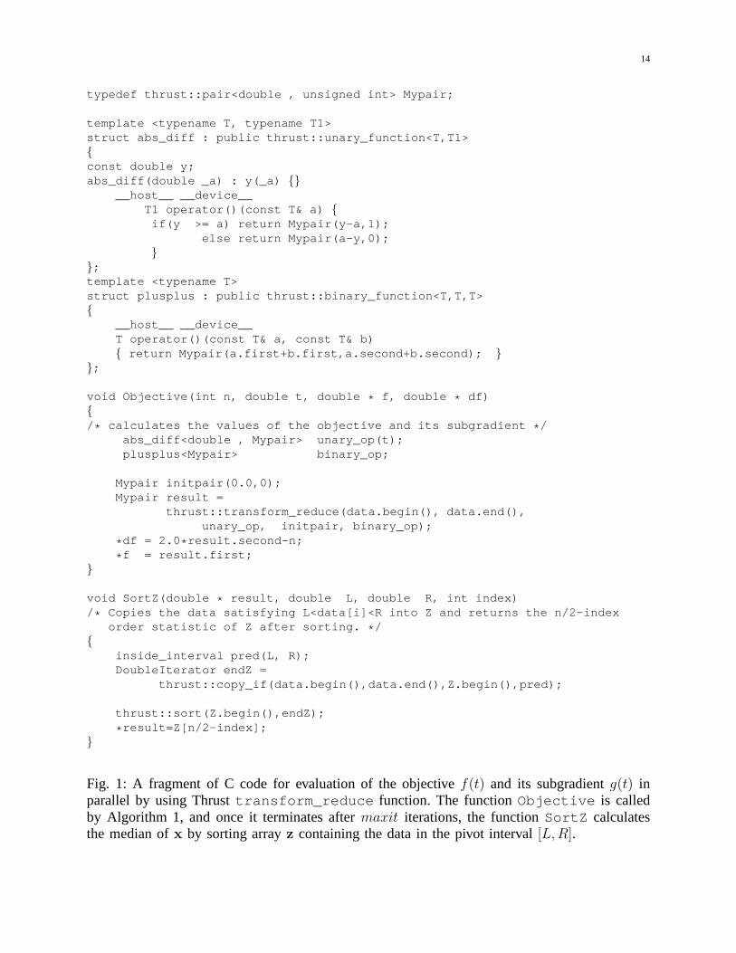
We outline the program code used to calculate the the objective f and its subgradientg neededby Algorithm 1 in Figure 1. The actual implementation of our algorithm calledcp_select li-brary, can be downloaded fromhttp://www.deakin.edu.au/∼gleb/cp_select.html.We want to stress the simplicity of the algorithm, which takes only a few lines of code relying on ahigh-level interface to standard algorithms, such as reduction and conditional copy, implementedin the Thrust library.

8

C. Empirical results

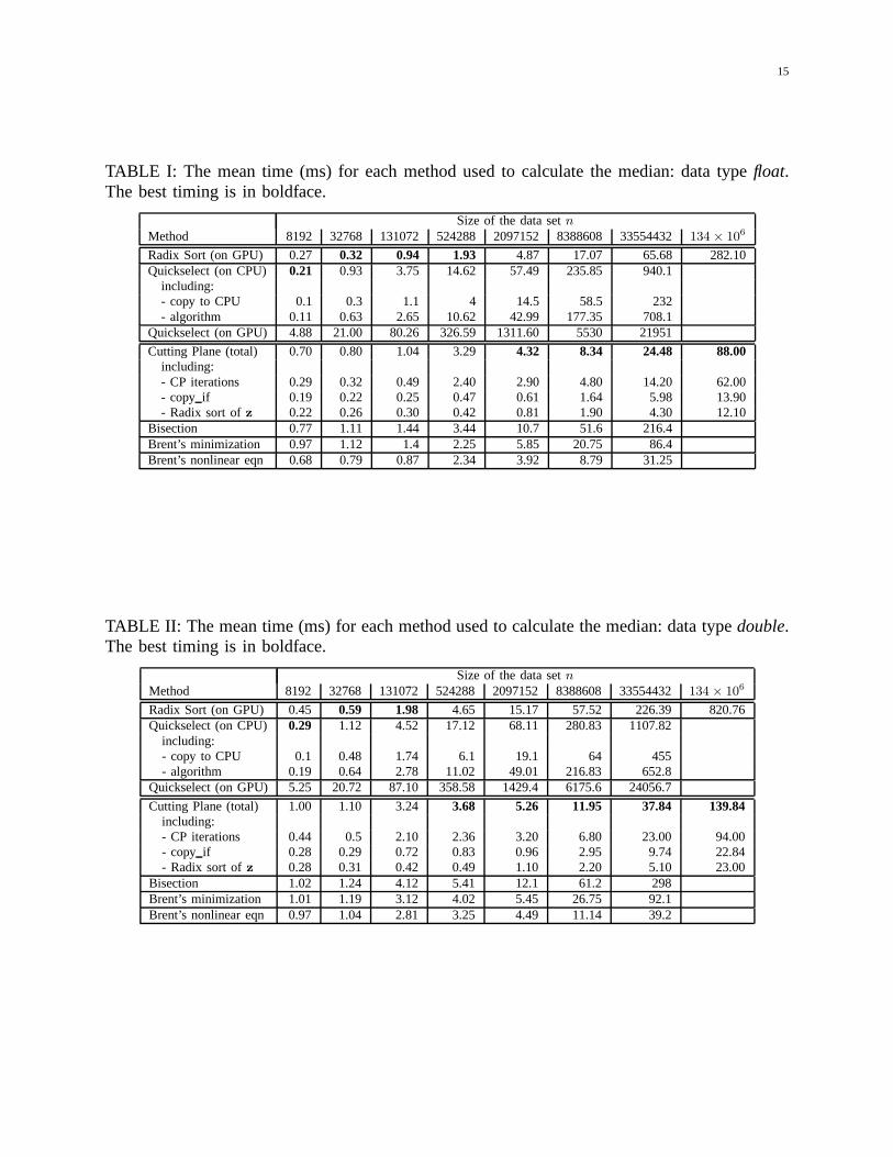
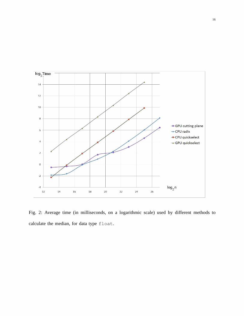
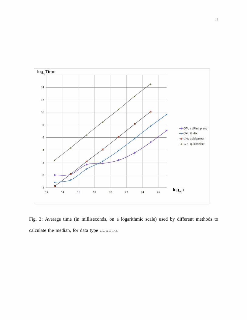
We present the results of our numerical experiments in Tables I and II for single and doubleprecision respectively, and graphically in Figures 2,3 (the plot is the log-log plot). We presentthe average results for all distributions, because we did not observe any significant deviationsfrom the average values for different distributions of the data. In fact, for the most efficient GPUradix sort and the proposed method, CPU times were very consistent: the largest and the smallestCPU time were within less than 5% from the average values. Forquickselect(both CPU andGPU versions) the variations were larger, but we did not observe any pattern related to the typeof the distribution, only variations between the instancesof data from the same distribution.

We observe that the use ofquickselecton the CPU was more efficient only for the smallestdata set testedn = 8192, and that for larger data sets GPU radix sort was faster by a factor ofthirteen and five for single and double precision respectively. Both copying the data and actualselection algorithm on CPU have contributed to the cost ofquickselecton CPU. We see from thetables that the time spent on just copying the data to CPU was larger than that of GPU radix sortstarting fromn ≥ 215, and the same was true for the time used byquickselectalgorithm itself.Execution ofquickselecton GPU in a single thread was worse than the remaining alternativesby a very large factor.

GPU radix sort was the most efficient method for up ton = 221. At that point the methodsbased on minimization outperformed GPU radix sort and consistently remained more efficient forlarge data sets. It looks from the plots of the logarithms of CPU time, that starting fromn = 223

the CPU time behaved likeO(n) for all methods, and the difference was due to a constantfactor. The difference in performance of GPU radix sort and the proposed method was morepronounced for double precision values, as one would have expected, because the performanceof the radix sort depends on the number of bits in the key.

Among the methods of minimization/root finding, bisection was the slowest. Brent’s rootfinding algorithm delivered similar performance to the cutting plane method, but its performancedegraded when data contained very large outliers, as explained below.

The difference in CPU time between the fastest existing alternative GPU radix sort and ourcutting plane method is almost six-fold for large arraysn = 227 (double) and three-fold (singleprecision).

D. Discussion

We note that unlike traditional sorting and selection algorithms, our methods based on mini-mization and root-finding are not sensitive to how the data are organized in the arrayx (e.g., atrandom, pre-sorted, or sorted in inverse order). Indeed expression (1) is invariant with respectto permutations of the components ofx.

However, the performance of all algorithms based on minimization or solving nonlinear equa-tions, except the cutting plane method, drastically decreased when just one or a few componentsof x took very large values (e.g.,109), which could happen in our application. We do not reportthe CPU times, because they depend on how large was the outlier. In fact we could slow downthe mentioned algorithms to any degree by taking a sufficiently large outlier. That is, all of ourmethods except cutting plane, are sensitive to the values ofxi. The reason is the following.

9

Clearly, the number of iterations of the bisection method required to achieve a fixed accuracyis O(log r), wherer = x(n)−x(1) is the range of the data, which can be unbounded. The same istrue for the golden section optimization method, which is the counterpart of the bisection. BothBrent’s methods reverted to the slower bisection/golden section methods because the objectiveis linear in almost all of the range of the data whenxi have such an uneven distribution. Hencethe parabolic fits attempted by Brent’s method are unsuccessful, see Figure 5.

The only optimization method insensitive to very large (or small) values ofxi was Kelley’scutting plane method. The reason this method was successfulis that it uses not only the valuesof the objective but also its subgradients, as well as convexity of the objective. The cutting planemethod iteratively builds a lower piecewise linear approximation to the objective, which alsohappens to be piecewise linear. In that way, just one value ofthe objective and its subgradientallows the algorithm to eliminate large uninteresting linear pieces (such as the intervals betweena large outlierxi and the bulk of the data), which do not contain the minimizer.

However, even the cutting plane method had problems when some components ofx wereextremely large, of order of1020, because of finite precision of machine arithmetic. When sucha large value is accounted for in the sum (1), all the subsequent terms do not contribute to thesum because of loss of precision, even though their combinedvalue can be sufficiently large.This is a well known effect in numerical analysis.

To circumvent this issue we used the following approach. Theorder statistics, and the medianin particular, are invariant with respect to monotone transformations. Then we can transform theelements ofx by applying an increasing functionF componentwiseF (x) = (F (x1), . . . , F (xn)),calculate the median of the transformed arraymedF = Med(F (x)), and then takemed =F−1(medF ). In our work we used transformationF (t) = log(1 + t− x(1)). In this case the lossof accuracy in summation is eliminated.

As we mentioned in Section IV, the complexity of the cutting plane algorithm ismaxit + 1parallel reductions, plus the time spent on conditional copy and sorting a reduced arrayz. In allour experiments, the arrayz turned out to be significantly smaller thanx, typically between to1% and 5% of the length ofx. Even if, hypothetically,z is almost as large asx, the complexityof the proposed method is tied to the complexity of the GPU radix sort, because the use ofcutting plane adds only a fixed initial overhead. We were unable to design a data set whichwould lead to such a hypothetical case.

Finally, we will mention the situation where the data are distributed across several GPUs.Parallel sorting algorithms require transfers of data between GPUs, which has a non-negligiblecost, even when such transfers do not involve the CPU, and unified virtual addressing is used, asin CUDA 4.0. In contrast, calculation of (1) and its subgradient is embarrassingly parallel, andinvolves reductions executed independently on different GPUs. The partial sums from severalGPUs are added together on the CPU. It works in a similar way for multiple GPUs connectedto different hosts, which are in turn connected through MPI interface, as only small portions ofdata need to be transferred on few occasions (of course, we assume that the number of GPUs isnot large). Therefore we see the approach based on minimization as the most suitable alternativeto selection on multiple GPUs

10

VI. A PPLICATION TO ROBUST REGRESSION

Next we outline our motivating problem of high breakdown regression, the role of the medianfunction and our GPU based algorithm. We also mention another application from data analysiswhich requires multiple calculations of the order statistics.

We consider the classical linear regression problem: givena set of pairs(xi, yi), i = 1, . . . , n:xi ∈ ℜ

p, yi ∈ ℜ (data), and a set of linear modelsfθ : ℜp → ℜ parameterized by a vector ofparametersθ ∈ Ω ⊆ ℜp determine the parameter vectorθ∗, such thatfθ∗ fits the data best. Thelinear models are

yi = xi1θ1 + . . .+ xipθp + εi, i = 1, . . . , n, (3)

with xip = 1 for regression with an intercept term.xij = X ∈ ℜn×p is the matrix of explanatoryvariables andε is ann-vector of iid random errors with zero mean and unknown variance.

The goodness of fit is expressed in terms of either squared or absolute residualsri = fθ(xi)−yi,namely the weighted averages

∑ni=1wir

2i (the least squares (LS) regression), or

∑ni=1wi|ri| (the

least absolute deviations (LAD) regression).The LS and LAD problems are not robust to outliers: it is sufficient to take just one contami-

nated point with an extremely large or small value ofyi or xij to break the regression model. Thebreakdown point of the LS and LAD estimators, i.e., the proportion of data that can make theestimator’s bias arbitrarily large, is 0 (see books [19], [27]). To overcome the lack of robustnessof the LS and LAD estimators, Rousseeuw [25] introduced the Least Median of Squares (LMS)estimator based on the solution of

Minimize F (θ) = Med(ri(θ))2.

He also introduced the method of the least trimmed squares (LTS) [25], which is consideredsuperior to the LMS [26], [28]. Here the expression to be minimized is

Minimize F (θ) =h

∑

i=1

(r(i)(θ))2,

where the residuals are ordered in the increasing order|r(1)| ≤ |r(2)| ≤ . . . ≤ |r(n)|, andh =[(n+ p)/2].

In essence, in the LMS and LTS methods, half of the sample is discarded as potentialoutliers, and the model is fitted to the remaining half. This makes the estimator not sensitive tocontamination in up to a half of the data. Of course, the problem is to decide which half of thedata should be discarded, and this is very challenging.

Numerical computation of the LMS or LTS estimator involves multiple evaluations ofF (θ).We clearly see the need in an efficient evaluation of the median in the LMS method, which isthe motivation for this work. Next we also show that the median can simplify calculation of theLTS objective, even though it appears that the vector of residuals needs to be fully sorted.

We rewrite the LTS objective in this form

Minimize F (θ) =n

∑

i=1

ρ(|r(i)(θ)|2), (4)

11

with

ρ(t) =

1 if t < Med(r)ab

if t = Med(r)0 otherwise

The integersa and b are computed from the multiplicity of the median, i.e., the number ofcomponents ofr equal to the median. Consider the numbersbL = count(|ri| < Med(r)) andb = count(|ri| = Med(r)). In the LTS method takeh = n+1

2for odd n, andh = n

2for evenn.

Thenh = bL+a for somea ≤ b. Now if we takea andb calculated in this way in (4), the valueof F in (4) will be the sum of exactlyh smallest residuals, and will coincide withF in the LTSmethod. The values ofa and b are easily calculated once the median is known, on either CPU(in O(n) time) or GPU (inO(n

p+ log p) time) by reduction.

Hence, calculation of the median is also valuable for the LTSmethod, where partial sortingof the absolute residuals can be replaced with a cheaper method based on the median.

Another application which requires multiple calculationsof order statistics, and which is easilyparallelized for GPUs is the k-nearest neighbor method (kNN), which is used in both regressionand classification. In the case of regression, it consists inapproximating a function value atxby f(x) =

∑ki=1wifi, where the valuesfi are the ordinates of thek pointsx1, . . . ,xk closest

to x (in some metric, usually the Euclidean distance) andwi are the weights that are decreasingfunctions of the distancesdi = ||x−xi||. In the case of classification, the majority vote (amongthe k nearest neighbors) is applied to determine the predicted class of the query pointx.

The kNN method is suitable for parallelization on GPUs. The array of distancesd, can becalculated on GPUs in parallel inO(n

p) time. The usual approach to selecting thek nearest

neighbors is to sort the data according to the distance tox. However, one can do better by usingthek-th order statistic. Indeed, by adapting the functionρ in (4), we obtain an indicator function,which returns a non-zero value for those data(xi, fi) that are no further fromx than thek-orderstatisticd(k). Then the weighted sum ofk nearest neighbors is calculated by reduction. Thus,efficient parallel calculations ofk-order statistics is useful in the kNN method as well.

VII. CONCLUSION

We considered a classical selection problem and discussed various approaches to parallelcomputation of the median and order statistics on GPUs. We compared numerical performance ofseveral existing and proposed methods by using a number of data sets with standard and unusualdistributions, and found that the most efficient way to calculate the median is by minimizinga convex function using the cutting plane method, followed by sorting a reduced sample. Thisapproach is between three and six times more efficient than the fastest existing method basedon GPU radix sort, depending on the data type used.

The proposed algorithm is easy to implement using high-level interface to GPU programmingimplemented in Thrust library, which is bundled with the newest CUDA 4.0 release. It usesa standard reduction operation, which is efficiently implemented in Thrust. Furthermore, ourapproach is scalable to multiple GPU devices, as only a very small number of transfers of databetween GPU and CPU is required.

12

We outlined two applications in data analysis which requirean efficient calculation of themedians and order statistics. Both applications are easilyparallelized for GPUs, and benefitfrom an efficient GPU-based selection algorithm.

REFERENCES

[1] I. Al-Furiah, S. Aluru, S. Goil, and S. Ranka. Practical algorithms for selection on coarse-grained parallel computers.

IEEE Trans. on Parallel and Distributed Syst., 8:813–824, 1997.

[2] D. Bader. An improved, randomized algorithm for parallel selection with an experimental study.J. Parallel Distrib.

Comput., 64:1051 – 1059, 2004.

[3] A. Bagirov. A method for minimization of quasidifferentiable functions.Optimization Methods and Software, 17:31–60,

2002.

[4] M. Blum, R.W. Floyd, V. Watt, R.L. Rive, and R.E. Tarjan. Time bounds for selection.Journal of Computer and System

Sciences, 7:448–461, 1973.

[5] P.S. Bullen.Handbook of Means and Their Inequalities. Kluwer, Dordrecht, 2003.

[6] T. Calvo and G. Beliakov. Aggregation functions based onpenalties.Fuzzy Sets and Systems, 161:1420–1436, 2010.

[7] T. Calvo, R. Mesiar, and R. Yager. Quantitative weights and aggregation.IEEE Trans. on Fuzzy Systems, 12:62–69, 2004.

[8] D. Cederman and P. Tsigas. GPU-Quicksort: A practical quicksort algorithm for graphics processors.ACM Journal of

Experimental Algorithmics, 14:1.4.1–1.4.24, 2009.

[9] F.H. Clarke. Optimization and Nonsmooth Analysis. John Wiley, New York, 1983.

[10] V.F. Demyanov and A.M. Rubinov.Constructive Nonsmooth Analysis. Peter Lang, Frankfurt am Main, 1995.

[11] C. Gini. Le Medie. Unione Tipografico-Editorial Torinese, Milan (Russian translation, Srednie Velichiny, Statistica,

Moscow, 1970), 1958.

[12] N. K. Govindaraju, J. Gray, R. Kumar, and D. Manocha. GPUTera-Sort: High performance graphics coprocessor sorting

for large database management. InProc. 2006 ACM SIGMOD Intl Conf. on Management of Data, pages 325–336, 2006.

[13] N. K. Govindaraju, B. Lloyd, W. Wang, M. Lin, and D. Manocha. Fast computation of database operations using graphic

processors. InProc. 2004 ACM SIGMOD Intl Conf. on Management of Data, pages 215 – 226, 2004.

[14] S. Le Grand. Broad-phase collision detection with CUDA. In H. Nguyen, editor,GPU Gems 3, pages 697–721. Addison-

Wesley Professional, 2007.

[15] J. Hoberock and N. Bell. Thrust: A parallel template library, http://www.meganewtons.com/, 2010. Version 1.3.0.

[16] D. Jackson. Note on the median of a set of numbers.Bulletin of the Americam Math. Soc., 27:160–164, 1921.

13

[17] J.E. Kelley. The cutting-plane method for solving convex programs.J. of SIAM, 8:703–712, 1960.

[18] N. Leischner, V. Osipov, and P. Sanders. GPU samplesort. In IEEE International Parallel and Distributed Processing

Symposium, Atlanta, 2010. IEEE, DOI: 10.1109/IPDPS.2010.5470444.

[19] R. Maronna, R. Martin, and V. Yohai.Robust Statistics: Theory and Methods. Wiley, New York, 2006.

[20] D. Merrill and A. Grimshaw. Revisiting sorting for GPGPU stream architectures. Technical Report CS2010-03, University

of Virginia, Department of Computer Science, Charlottesville, VA, USA, 2010.

[21] NVIDIA. http://developer.download.nvidia.com/compute/cuda/11/website/data-parallelalgorithms.html, accessed 1 Feb,

2011.

[22] NVIDIA. http://developer.nvidia.com/object/cuda4 0 rc downloads.html, accessed 20 March, 2011.

[23] NVIDIA. Tesla datasheet, http://www.nvidia.com/docs/io/43395/ nvds tesla psc us nov08 lowres.pdf, accessed 1 De-

cember, 2010.

[24] A.H. Press, S.A. Teukolsky, W.T. Vetterling, and B.P. Flannery.Numerical Recipes in C: The Art of Scientific Computing.

Cambridge University Press, New York, 2002.

[25] P.J. Rousseeuw. Least median of squares regression.J. Amer. Statist. Assoc, 79:871–880, 1984.

[26] P.J. Rousseeuw and C. Croux. Alternatives to the medianabsolute deviation.J. Amer. Statist. Assoc, 88:1273–1283, 1993.

[27] P.J. Rousseeuw and A.M. Leroy.Robust Regression and Outlier Detection. Wiley, New York, 2003.

[28] P.J. Rousseeuw and K. Van Driessen. Computing lts regression for large data sets.Data Mining and Knowledge Discovery,

12:29–45, 2006.

[29] N. Satish, M. Harris, and M. Garland. Designing efficient sorting algorithms for manycore GPUs. InIn Proc. of IEEE

Intl Parallel and Distributed Processing Symposium (IPDPS2009), Rome, DOI: 10.1109/IPDPS.2009.5161005, 2009.

[30] E.L. Saukas and S.W. Song. Efficient selection algorithms on distributed memory computers. InACM/IEEE Conference

on Supercomputing, pages 1–26, San Jose, CA, 1998. IEEE.

[31] R. Sedgewick.Algorithms. Addison-Wesley, Reading, MA, 2nd edition, 1988.

[32] S. Sengupta, M. Harris, Y. Zhang, and J. D. Owens. Scan primitives for GPU computing.Graphics Hardware, pages

97–106, 2007.

[33] E. Sintorn and U. Assarsson. Fast parallel GPU-sortingusing a hybrid algorithm.J. of Parallel and Distributed Computing,

68:1381–1388, 2008.

[34] A. Tiskin. Parallel selection by regular sampling.LNCS, 6272:393–399, 2009.

[35] R. Yager and A. Rybalov. Understanding the median as a fusion operator.Int. J. General Syst., 26:239–263, 1997.

14

typedef thrust::pair<double , unsigned int> Mypair;

template <typename T, typename T1>struct abs_diff : public thrust::unary_function<T,T1>const double y;abs_diff(double _a) : y(_a)

__host__ __device__T1 operator()(const T& a) if(y >= a) return Mypair(y-a,1);

else return Mypair(a-y,0);

;template <typename T>struct plusplus : public thrust::binary_function<T,T,T>

__host__ __device__T operator()(const T& a, const T& b) return Mypair(a.first+b.first,a.second+b.second);

;

void Objective(int n, double t, double * f, double * df)/* calculates the values of the objective and its subgradient */

abs_diff<double , Mypair> unary_op(t);plusplus<Mypair> binary_op;

Mypair initpair(0.0,0);Mypair result =

thrust::transform_reduce(data.begin(), data.end(),unary_op, initpair, binary_op);

*df = 2.0*result.second-n;

*f = result.first;

void SortZ(double * result, double L, double R, int index)/* Copies the data satisfying L<data[i]<R into Z and returns the n/2-index

order statistic of Z after sorting. */

inside_interval pred(L, R);DoubleIterator endZ =

thrust::copy_if(data.begin(),data.end(),Z.begin(),pred);

thrust::sort(Z.begin(),endZ);

*result=Z[n/2-index];

Fig. 1: A fragment of C code for evaluation of the objectivef(t) and its subgradientg(t) inparallel by using Thrusttransform_reduce function. The functionObjective is calledby Algorithm 1, and once it terminates aftermaxit iterations, the functionSortZ calculatesthe median ofx by sorting arrayz containing the data in the pivot interval[L,R].

15

TABLE I: The mean time (ms) for each method used to calculate the median: data typefloat.The best timing is in boldface.

Size of the data setnMethod 8192 32768 131072 524288 2097152 8388608 33554432 134× 10

6

Radix Sort (on GPU) 0.27 0.32 0.94 1.93 4.87 17.07 65.68 282.10Quickselect (on CPU) 0.21 0.93 3.75 14.62 57.49 235.85 940.1

including:- copy to CPU 0.1 0.3 1.1 4 14.5 58.5 232- algorithm 0.11 0.63 2.65 10.62 42.99 177.35 708.1

Quickselect (on GPU) 4.88 21.00 80.26 326.59 1311.60 5530 21951

Cutting Plane (total) 0.70 0.80 1.04 3.29 4.32 8.34 24.48 88.00including:- CP iterations 0.29 0.32 0.49 2.40 2.90 4.80 14.20 62.00- copy if 0.19 0.22 0.25 0.47 0.61 1.64 5.98 13.90- Radix sort ofz 0.22 0.26 0.30 0.42 0.81 1.90 4.30 12.10

Bisection 0.77 1.11 1.44 3.44 10.7 51.6 216.4Brent’s minimization 0.97 1.12 1.4 2.25 5.85 20.75 86.4Brent’s nonlinear eqn 0.68 0.79 0.87 2.34 3.92 8.79 31.25

TABLE II: The mean time (ms) for each method used to calculatethe median: data typedouble.The best timing is in boldface.

Size of the data setnMethod 8192 32768 131072 524288 2097152 8388608 33554432 134× 10

6

Radix Sort (on GPU) 0.45 0.59 1.98 4.65 15.17 57.52 226.39 820.76Quickselect (on CPU) 0.29 1.12 4.52 17.12 68.11 280.83 1107.82

including:- copy to CPU 0.1 0.48 1.74 6.1 19.1 64 455- algorithm 0.19 0.64 2.78 11.02 49.01 216.83 652.8

Quickselect (on GPU) 5.25 20.72 87.10 358.58 1429.4 6175.6 24056.7

Cutting Plane (total) 1.00 1.10 3.24 3.68 5.26 11.95 37.84 139.84including:- CP iterations 0.44 0.5 2.10 2.36 3.20 6.80 23.00 94.00- copy if 0.28 0.29 0.72 0.83 0.96 2.95 9.74 22.84- Radix sort ofz 0.28 0.31 0.42 0.49 1.10 2.20 5.10 23.00

Bisection 1.02 1.24 4.12 5.41 12.1 61.2 298Brent’s minimization 1.01 1.19 3.12 4.02 5.45 26.75 92.1Brent’s nonlinear eqn 0.97 1.04 2.81 3.25 4.49 11.14 39.2

16

Fig. 2: Average time (in milliseconds, on a logarithmic scale) used by different methods to

calculate the median, for data typefloat.

17

Fig. 3: Average time (in milliseconds, on a logarithmic scale) used by different methods to

calculate the median, for data typedouble.

18

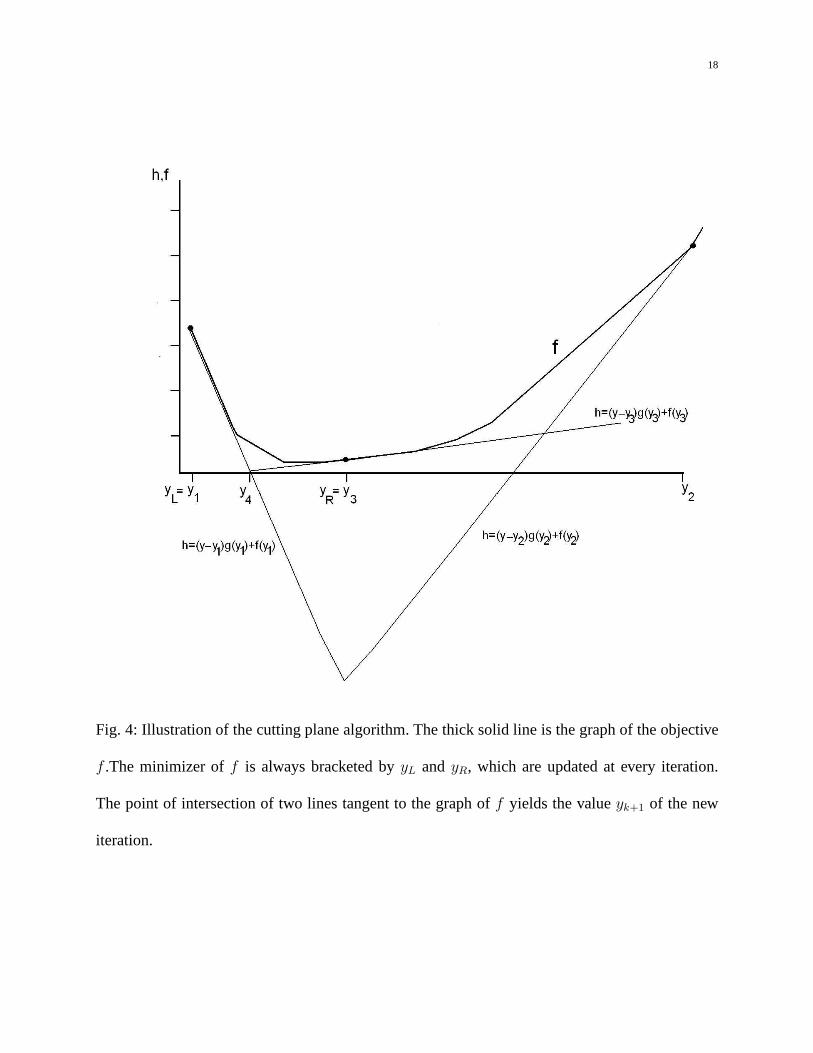
Fig. 4: Illustration of the cutting plane algorithm. The thick solid line is the graph of the objective

f .The minimizer off is always bracketed byyL and yR, which are updated at every iteration.

The point of intersection of two lines tangent to the graph off yields the valueyk+1 of the new

iteration.

19

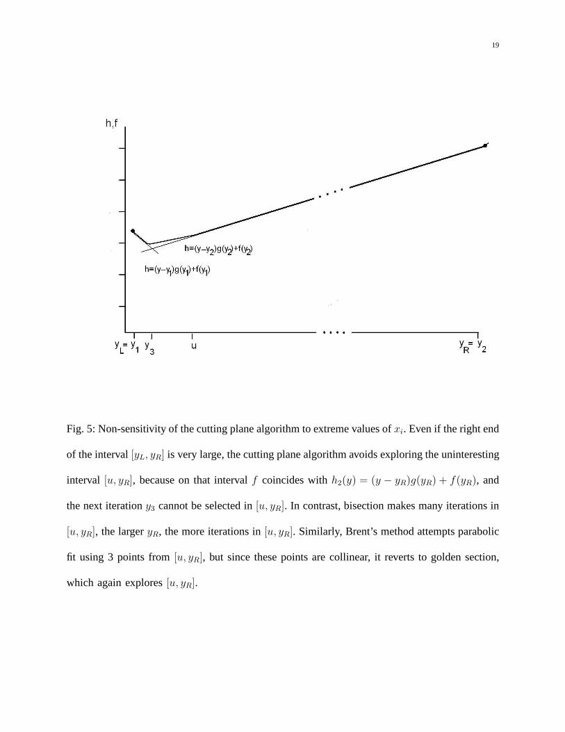
Fig. 5: Non-sensitivity of the cutting plane algorithm to extreme values ofxi. Even if the right end

of the interval[yL, yR] is very large, the cutting plane algorithm avoids exploringthe uninteresting

interval [u, yR], because on that intervalf coincides withh2(y) = (y − yR)g(yR) + f(yR), and

the next iterationy3 cannot be selected in[u, yR]. In contrast, bisection makes many iterations in

[u, yR], the largeryR, the more iterations in[u, yR]. Similarly, Brent’s method attempts parabolic

fit using 3 points from[u, yR], but since these points are collinear, it reverts to golden section,

which again explores[u, yR].