Embed Size (px)
Citation preview
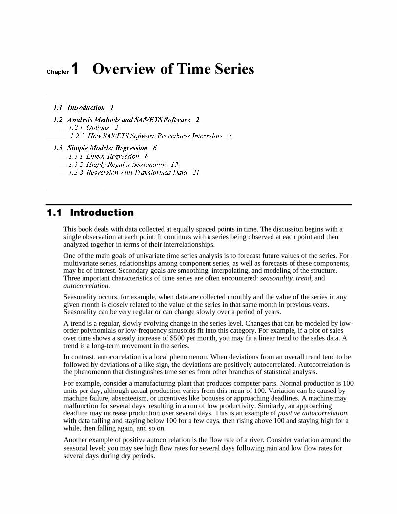
Chapter 1 Overview of Time Series
1.1 Introduction 1
1.2 Analysis Methods and SAS/ETS Software 2
1.2.1 Options 2
1.2.2 How SAS/ETS Software Procedures Interrelate 4
1.3 Simple Models: Regression 6
1.3.1 Linear Regression 6
1.3.2 Highly Regular Seasonality 13
1.3.3 Regression with Transformed Data 21
1.1 Introduction
This book deals with data collected at equally spaced points in time. The discussion begins with a single observation at each point. It continues with k series being observed at each point and then analyzed together in terms of their interrelationships.
One of the main goals of univariate time series analysis is to forecast future values of the series. For multivariate series, relationships among component series, as well as forecasts of these components, may be of interest. Secondary goals are smoothing, interpolating, and modeling of the structure. Three important characteristics of time series are often encountered: seasonality, trend, and autocorrelation.
Seasonality occurs, for example, when data are collected monthly and the value of the series in any given month is closely related to the value of the series in that same month in previous years. Seasonality can be very regular or can change slowly over a period of years.
A trend is a regular, slowly evolving change in the series level. Changes that can be modeled by low-order polynomials or low-frequency sinusoids fit into this category. For example, if a plot of sales over time shows a steady increase of $500 per month, you may fit a linear trend to the sales data. A trend is a long-term movement in the series.
In contrast, autocorrelation is a local phenomenon. When deviations from an overall trend tend to be followed by deviations of a like sign, the deviations are positively autocorrelated. Autocorrelation is the phenomenon that distinguishes time series from other branches of statistical analysis.
For example, consider a manufacturing plant that produces computer parts. Normal production is 100 units per day, although actual production varies from this mean of 100. Variation can be caused by machine failure, absenteeism, or incentives like bonuses or approaching deadlines. A machine may malfunction for several days, resulting in a run of low productivity. Similarly, an approaching deadline may increase production over several days. This is an example of positive autocorrelation, with data falling and staying below 100 for a few days, then rising above 100 and staying high for a while, then falling again, and so on.
Another example of positive autocorrelation is the flow rate of a river. Consider variation around the seasonal level: you may see high flow rates for several days following rain and low flow rates for several days during dry periods.
2 SAS for Forecasting Time Series
Negative autocorrelation occurs less often than positive autocorrelation. An example is a worker's attempt to control temperature in a furnace. The autocorrelation pattern depends on the worker's habits, but suppose he reads a low value of a furnace temperature and turns up the heat too far and similarly turns it down too far when readings are high. If he reads and adjusts the temperature each minute, you can expect a low temperature reading to be followed by a high reading. As a second example, an athlete may follow a long workout day with a short workout day and vice versa. The time he spends exercising daily displays negative autocorrelation.
1.2 Analysis Methods and SAS/ETS Software
1.2.1 Options When you perform univariate time series analysis, you observe a single series over time. The goal is to model the historic series and then to use the model to forecast future values of the series. You can use some simple SAS/ETS software procedures to model low-order polynomial trends and autocorrelation. PROC FORECAST automatically fits an overall linear or quadratic trend with autoregressive (AR) error structure when you specify METHOD=STEPAR. As explained later, AR errors are not the most general types of errors that analysts study. For seasonal data you may want to fit a Winters exponentially smoothed trend-seasonal model with METHOD=WINTERS. If the trend is local, you may prefer METHOD=EXPO, which uses exponential smoothing to fit a local linear or quadratic trend. For higher-order trends or for cases where the forecast variable Y
t is related to one or
more explanatory variables Xt, PROC AUTOREG estimates this relationship and fits an AR series as
an error term.
Polynomials in time and seasonal indicator variables (see Section 1.3.2) can be computed as far into the future as desired. If the explanatory variable is a nondeterministic time series, however, actual future values are not available. PROC AUTOREG treats future values of the explanatory variable as known, so user-supplied forecasts of future values with PROC AUTOREG may give incorrect standard errors of forecast estimates. More sophisticated procedures like PROC STATESPACE, PROC VARMAX, or PROC ARIMA, with their transfer function options, are preferable when the explanatory variable's future values are unknown.
One approach to modeling seasonality in time series is the use of seasonal indicator variables in PROC AUTOREG to model a highly regular seasonality. Also, the AR error series from PROC AUTOREG or from PROC FORECAST with METHOD=STEPAR can include some correlation at seasonal lags (that is, it may relate the deviation from trend at time t to the deviation at time t−12 in monthly data). The WINTERS method of PROC FORECAST uses updating equations similar to exponential smoothing to fit a seasonal multiplicative model.
Another approach to seasonality is to remove it from the series and to forecast the seasonally adjusted series with other seasonally adjusted series used as inputs, if desired. The U.S. Census Bureau has adjusted thousands of series with its X-11 seasonal adjustment package. This package is the result of years of work by census researchers and is the basis for the seasonally adjusted figures that the federal government reports. You can seasonally adjust your own data using PROC X11, which is the census program set up as a SAS procedure. If you are using seasonally adjusted figures as explanatory variables, this procedure is useful.
Chapter 1: Overview of Time Series 3
An alternative to using X-11 is to model the seasonality as part of an ARIMA model or, if the seasonality is highly regular, to model it with indicator variables or trigonometric functions as explanatory variables. A final introductory point about the PROC X11 program is that it identifies and adjusts for outliers.*
If you are unsure about the presence of seasonality, you can use PROC SPECTRA to check for it; this procedure decomposes a series into cyclical components of various periodicities. Monthly data with highly regular seasonality have a large ordinate at period 12 in the PROC SPECTRA output SAS data set. Other periodicities, like multiyear business cycles, may appear in this analysis. PROC SPECTRA also provides a check on model residuals to see if they exhibit cyclical patterns over time. Often these cyclical patterns are not found by other procedures. Thus, it is good practice to analyze residuals with this procedure. Finally, PROC SPECTRA relates an output time series Y
t to one or
more input or explanatory series Xt in terms of cycles. Specifically, cross-spectral analysis estimates
the change in amplitude and phase when a cyclical component of an input series is used to predict the corresponding component of an output series. This enables the analyst to separate long-term movements from short-term movements.
Without a doubt, the most powerful and sophisticated methodology for forecasting univariate series is the ARIMA modeling methodology popularized by Box and Jenkins (1976). A flexible class of models is introduced, and one member of the class is fit to the historic data. Then the model is used to forecast the series. Seasonal data can be accommodated, and seasonality can be local; that is, seasonality for month t may be closely related to seasonality for this same month one or two years previously but less closely related to seasonality for this month several years previously. Local trending and even long-term upward or downward drifting in the data can be accommodated in ARIMA models through differencing.
Explanatory time series as inputs to a transfer function model can also be accommodated. Future values of nondeterministic, independent input series can be forecast by PROC ARIMA, which, unlike the previously mentioned procedures, accounts for the fact that these inputs are forecast when you compute prediction error variances and prediction limits for forecasts. A relatively new procedure, PROC VARMAX, models vector processes with possible explanatory variables, the X in VARMAX. As in PROC STATESPACE, this approach assumes that at each time point you observe a vector of responses each entry of which depends on its own lagged values and lags of the other vector entries, but unlike STATESPACE, VARMAX also allows explanatory variables X as well as cointegration among the elements of the response vector. Cointegration is an idea that has become quite popular in recent econometrics. The idea is that each element of the response vector might be a nonstationary process, one that has no tendency to return to a mean or deterministic trend function, and yet one or more linear combinations of the responses are stationary, remaining near some constant. An analogy is two lifeboats adrift in a stormy sea but tied together by a rope. Their location might be expressible mathematically as a random walk with no tendency to return to a particular point. Over time the boats drift arbitrarily far from any particular location. Nevertheless, because they are tied together, the difference in their positions would never be too far from 0. Prices of two similar stocks might, over time, vary according to a random walk with no tendency to return to a given mean, and yet if they are indeed similar, their price difference may not get too far from 0.
* Recently the Census Bureau has upgraded X-11, including an option to extend the series using ARIMA models prior to applying the centered filters used to deseasonalize the data. The resulting X-12 is incorporated as PROC X12 in SAS software.
4 SAS for Forecasting Time Series
1.2.2 How SAS/ETS Software Procedures Interrelate PROC ARIMA emulates PROC AUTOREG if you choose not to model the inputs. ARIMA can also fit a richer error structure. Specifically, the error structure can be an autoregressive (AR), moving average (MA), or mixed-model structure. PROC ARIMA can emulate PROC FORECAST with METHOD=STEPAR if you use polynomial inputs and AR error specifications. However, unlike FORECAST, ARIMA provides test statistics for the model parameters and checks model adequacy. PROC ARIMA can emulate PROC FORECAST with METHOD=EXPO if you fit a moving average of order d to the dth difference of the data. Instead of arbitrarily choosing a smoothing constant, as necessary in PROC FORECAST METHOD=EXPO, the data tell you what smoothing constant to use when you invoke PROC ARIMA. Furthermore, PROC ARIMA produces more reasonable forecast intervals. In short, PROC ARIMA does everything the simpler procedures do and does it better.
However, to benefit from this additional flexibility and sophistication in software, you must have enough expertise and time to analyze the series. You must be able to identify and specify the form of the time series model using the autocorrelations, partial autocorrelations, inverse autocorrelations, and cross-correlations of the time series. Later chapters explain in detail what these terms mean and how to use them. Once you identify a model, fitting and forecasting are almost automatic.
The identification process is more complicated when you use input series. For proper identification, the ARIMA methodology requires that inputs be independent of each other and that there be no feedback from the output series to the input series. For example, if the temperature T
t in a room at
time t is to be explained by current and lagged furnace temperatures Ft, lack of feedback corresponds
to there being no thermostat in the room. A thermostat causes the furnace temperature to adjust to recent room temperatures. These ARIMA restrictions may be unrealistic in many examples. You can use PROC STATESPACE and PROC VARMAX to model multiple time series without these restrictions.
Although PROC STATESPACE and PROC VARMAX are sophisticated in theory, they are easy to run in their default mode. The theory allows you to model several time series together, accounting for relationships of individual component series with current and past values of the other series. Feedback and cross-correlated input series are allowed. Unlike PROC ARIMA, PROC STATESPACE uses an information criterion to select a model, thus eliminating the difficult identification process in PROC ARIMA. For example, you can put data on sales, advertising, unemployment rates, and interest rates into the procedure and automatically produce forecasts of these series. It is not necessary to intervene, but you must be certain that you have a property known as stationarity in your series to obtain theoretically valid results. The stationarity concept is discussed in Chapter 3, “The General ARIMA Model,” where you will learn how to make nonstationary series stationary.
Although the automatic modeling in PROC STATESPACE sounds appealing, two papers in the Proceedings of the Ninth Annual SAS Users Group International Conference (one by Bailey and the other by Chavern) argue that you should use such automated procedures cautiously. Chavern gives an example in which PROC STATESPACE, in its default mode, fails to give as accurate a forecast as a certain vector autoregression. (However, the stationarity of the data is questionable, and stationarity is required to use PROC STATESPACE appropriately.) Bailey shows a PROC STATESPACE
Chapter 1: Overview of Time Series 5
forecast considerably better than its competitors in some time intervals but not in others. In SAS Views: SAS Applied Time Series Analysis and Forecasting, Brocklebank and Dickey generate data from a simple MA model and feed these data into PROC STATESPACE in the default mode. The dimension of the model is overestimated when 50 observations are used, but the procedure is successful for samples of 100 and 500 observations from this simple series. Thus, it is wise to consider intervening in the modeling procedure through PROC STATESPACE’s control options. If a transfer function model is appropriate, PROC ARIMA is a viable alternative.
This chapter introduces some techniques for analyzing and forecasting time series and lists the SAS procedures for the appropriate computations. As you continue reading the rest of the book, you may want to refer back to this chapter to clarify the relationships among the various procedures.
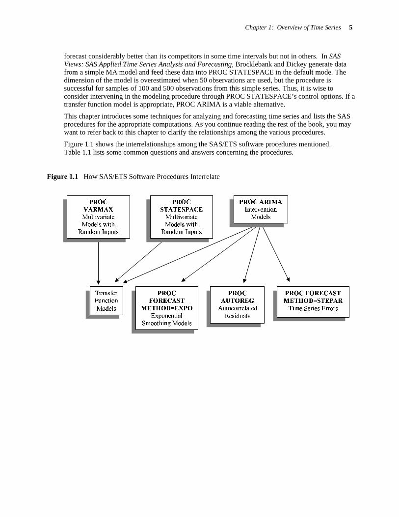
Figure 1.1 shows the interrelationships among the SAS/ETS software procedures mentioned. Table 1.1 lists some common questions and answers concerning the procedures.
Figure 1.1 How SAS/ETS Software Procedures Interrelate
PROC
STATESPACE
Multivariate
Models with Random Inputs
PROC ARIMA Intervention
Models
Transfer
Function
Models
PROC
FORECAST
METHOD=EXPO
Exponential
Smoothing Models
PROC
AUTOREG
Autocorrelated
Residuals
PROC FORECAST
METHOD=STEPAR
Time Series Errors
PROC
VARMAX
Multivariate
Models with Random Inputs
6 SAS for Forecasting Time Series
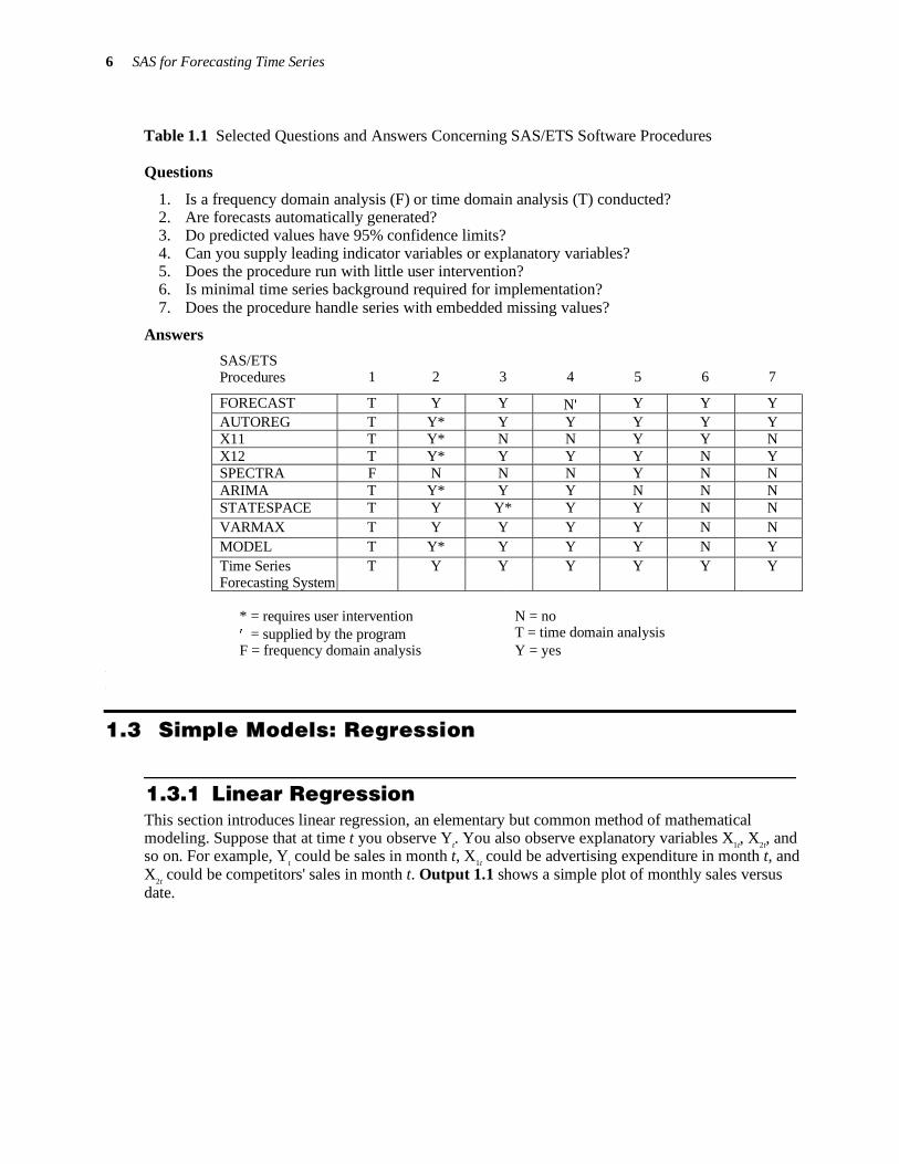
Table 1.1 Selected Questions and Answers Concerning SAS/ETS Software Procedures
Questions
1. Is a frequency domain analysis (F) or time domain analysis (T) conducted? 2. Are forecasts automatically generated? 3. Do predicted values have 95% confidence limits? 4. Can you supply leading indicator variables or explanatory variables? 5. Does the procedure run with little user intervention? 6. Is minimal time series background required for implementation? 7. Does the procedure handle series with embedded missing values?
Answers
SAS/ETS Procedures 1 2 3 4 5 6 7
FORECAST T Y Y N′ Y Y Y AUTOREG T Y* Y Y Y Y Y X11 T Y* N N Y Y N X12 T Y* Y Y Y N Y SPECTRA F N N N Y N N ARIMA T Y* Y Y N N N STATESPACE T Y Y* Y Y N N VARMAX T Y Y Y Y N N MODEL T Y* Y Y Y N Y Time Series Forecasting System
T Y Y Y Y Y Y
* = requires user intervention
N = no
′ = supplied by the program T = time domain analysis F = frequency domain analysis Y = yes
1.3 Simple Models: Regression
1.3.1 Linear Regression This section introduces linear regression, an elementary but common method of mathematical modeling. Suppose that at time t you observe Y
t. You also observe explanatory variables X
1t, X
2t, and
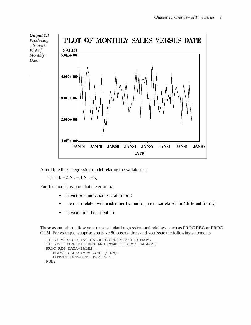
so on. For example, Yt could be sales in month t, X
1t could be advertising expenditure in month t, and
X2t could be competitors' sales in month t. Output 1.1 shows a simple plot of monthly sales versus
date.
Chapter 1: Overview of Time Series 7
Output 1.1 Producing a Simple Plot of Monthly Data
A multiple linear regression model relating the variables is
0 1 1 2 2Y X X
t t t t= β +β + β + ε
For this model, assume that the errors t
ε
• have the same variance at all times t
• are uncorrelated with each other (t
ε and s
ε are uncorrelated for t different from s)
• have a normal distribution.
These assumptions allow you to use standard regression methodology, such as PROC REG or PROC GLM. For example, suppose you have 80 observations and you issue the following statements:
TITLE “PREDICTING SALES USING ADVERTISING”; TITLE2 “EXPENDITURES AND COMPETITORS’ SALES”; PROC REG DATA=SALES; MODEL SALES=ADV COMP / DW;
OUTPUT OUT=OUT1 P=P R=R; RUN;
8 SAS for Forecasting Time Series
PREDICTING SALES USING ADVERTISING EXPENDITURES AND COMPETITORS' SALES
The REG Procedure Model: MODEL1
Dependent Variable: SALES
Analysis of Variance
Sum of Mean Source DF Squares Square F Value Prob>F
Model 2 2.5261822E13 1.2630911E13 51.140 0.0001 Error 77 1.9018159E13 246989077881
C Total 79 4.427998E13
Root MSE 496979.95722 R-square 0.5705
Dep Mean 3064722.70871 Adj R-sq 0.5593
C.V. 16.21615
Parameter Estimates
� Parameter � Standard T for H0:
Variable DF Estimate Error Parameter=0 Prob > |T|
INTERCEP 1 2700165 373957.39855 7.221 0.0001
ADV 1 10.179675 1.91704684 5.310 0.0001
COMP 1 -0.605607 0.08465433 -7.154 0.0001
Durbin-Watson D 1.394 �
(For Number of Obs.) 80 1st Order Autocorrelation 0.283 �
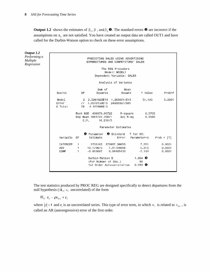
Output 1.2 shows the estimates of 210
and,, βββ �. The standard errors � are incorrect if the
assumptions on t
ε are not satisfied. You have created an output data set called OUT1 and have called for the Durbin-Watson option to check on these error assumptions.
Output 1.2 Performing a Multiple Regression
The test statistics produced by PROC REG are designed specifically to detect departures from the null hypothesis (
tε:H
0 uncorrelated) of the form
ttte+ρε=ε
−11:H
where 1<ρ and et is an uncorrelated series. This type of error term, in which
tε is related to
1−ε
t, is
called an AR (autoregressive) error of the first order.
Chapter 1: Overview of Time Series 9
The Durbin-Watson option in the MODEL statement produces the Durbin-Watson test statistic �
( )2
2
2 1 1ˆ ˆ ˆ/
n n
t t t t td
= − =
= Σ ε − ε Σ ε
where
0 1 1 2 2
ˆ ˆ ˆˆ Y X Xt t t tε = − β − β − β
If the actual errors t
ε are uncorrelated, the numerator of d has an expected value of about ( ) 212 σ−n
and the denominator has an expected value of approximately 2σn . Thus, if the errors
tε are
uncorrelated, the ratio d should be approximately 2.
Positive autocorrelation means that t
ε is closer to 1−
εt
than in the independent case, so 1−
ε−εtt
should be smaller. It follows that d should also be smaller. The smallest possible value for d is 0. If d is significantly less than 2, positive autocorrelation is present.
When is a Durbin-Watson statistic significant? The answer depends on the number of coefficients in the regression and on the number of observations. In this case, you have k=3 coefficients (
0 1 2and, ,β β β for the intercept, ADV, and COMP) and n=80 observations. In general, if you want
to test for positive autocorrelation at the 5% significance level, you must compare d=2.046 to a critical value. Even with k and n fixed, the critical value can vary depending on actual values of the independent variables. The results of Durbin and Watson imply that if k=3 and n=80, the critical value must be between d
L=1.59 and d
U=1.69. If d is less than d
L, then you would reject the null
hypotheses of uncorrelated errors in favor of the alternative: positive autocorrelation. Since d>2, which is evidence of negative autocorrelation, compute d′=4–d and compare the results to d
L and d
U.
Specifically, because d′ (1.954) is greater than 1.69, you are unable to reject the null hypothesis of uncorrelated errors. If d′ were less than 1.59 you would reject the null hypothesis of uncorrelated errors in favor of the alternative: negative autocorrelation. Note that if
1.59 < d < 1.69
you cannot be sure whether d is to the left or right of the actual critical value c because you know only that
1.59 < c < 1.69
Durbin and Watson have constructed tables of bounds for the critical values. Most tables use k′=k−1, which equals the number of explanatory variables, excluding the intercept and n (number of observations) to obtain the bounds d
L and d
U for any given regression (Draper and Smith 1998).*
Three warnings apply to the Durbin-Watson test. First, it is designed to detect first-order AR errors. Although this type of autocorrelation is only one possibility, it seems to be the most common. The test has some power against other types of autocorrelation. Second, the Durbin-Watson bounds do not hold when lagged values of the dependent variable appear on the right side of the regression. Thus, if the example had used last month's sales to help explain this month's sales, you would not know correct bounds for the critical value. Third, if you incorrectly specify the model, the Durbin-Watson statistic often lies in the critical region even though no real autocorrelation is present. Suppose an important variable, such as X
3t=product availability, had been omitted in the sales
example. This omission could produce a significant d. Some practitioners use d as a lack-of-fit statistic, which is justified only if you assume a priori that a correctly specified model cannot have autocorrelated errors and, thus, that significance of d must be due to lack of fit.
* Exact p-values for d are now available in PROC AUTOREG as will be seen in Output 1.2A later in this section.
10 SAS for Forecasting Time Series
The output also produced a first-order autocorrelation, � denoted as
ˆ 0.283ρ =
When n is large and the errors are uncorrelated,
( )1/ 2
1/ 2 2ˆ ˆ/ 1n ρ − ρ
is approximately distributed as a standard normal variate. Thus, a value
( )1/ 2
1/ 2 2ˆ ˆ/ 1n ρ − ρ
exceeding 1.645 is significant evidence of positive autocorrelation at the 5% significance level. This is especially helpful when the number of observations exceeds the largest in the Durbin-Watson table—for example,
80 (.283)/ 2283.01− = 2.639
You should use this test only for large n values. It is subject to the three warnings given for the
Durbin-Watson test. Because of the approximate nature of the ( )1/ 2
1/ 2 2ˆ ˆ/ 1n ρ − ρ test, the Durbin-
Watson test is preferable. In general, d is approximately ( )ρ− ˆ12 .
This is easily seen by noting that
and
Durbin and Watson also gave a computer-intensive way to compute exact p-values for their test statistic d. This has been incorporated in PROC AUTOREG. For the sales data, you issue this code to fit a model for sales as a function of this-period and last-period advertising.
PROC AUTOREG DATA=NCSALES; MODEL SALES=ADV ADV1 / DWPROB;
RUN;
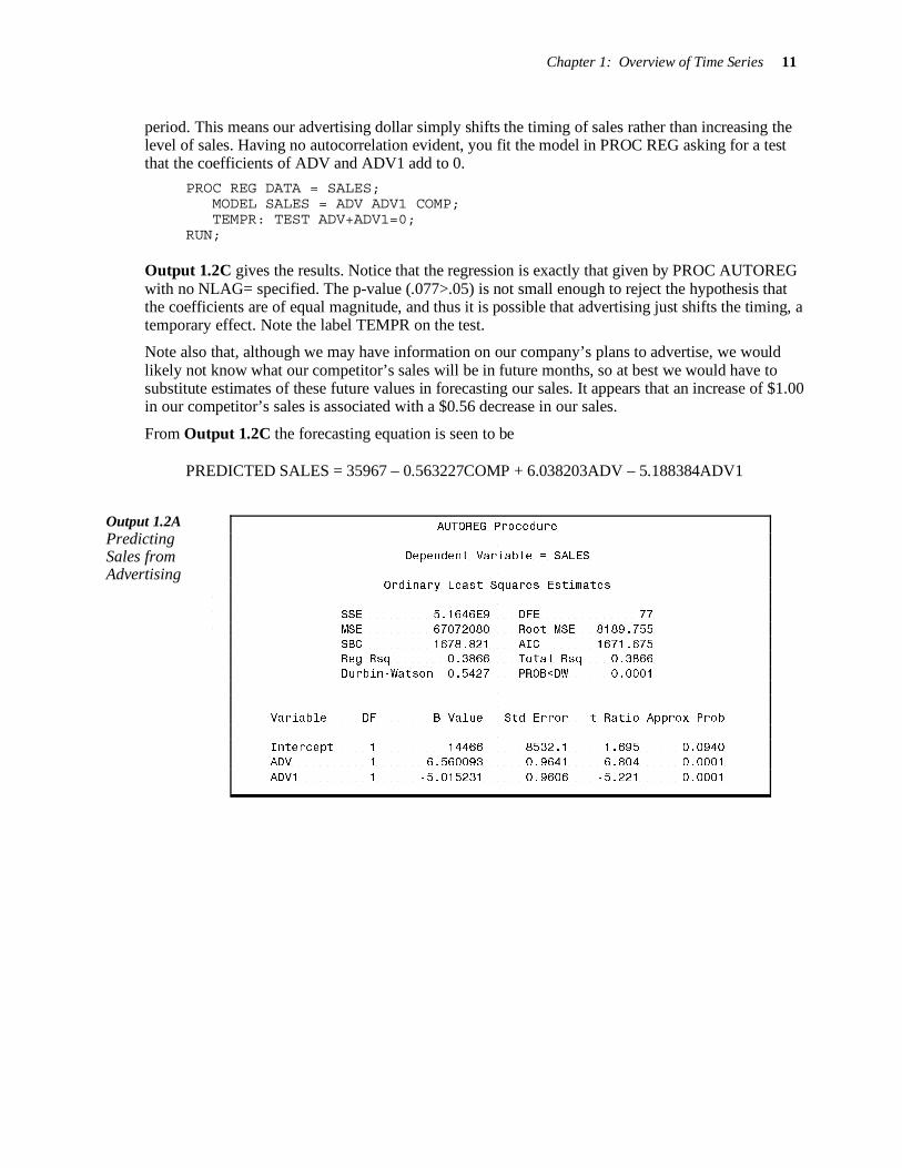
The resulting Output 1.2A shows a significant d=.5427 (p-value .0001 < .05). Could this be because of an omitted variable? Try the model with competitor’s sales included.
PROC AUTOREG DATA=NCSALES; MODEL SALES=ADV ADV1 COMP / DWPROB;
RUN;
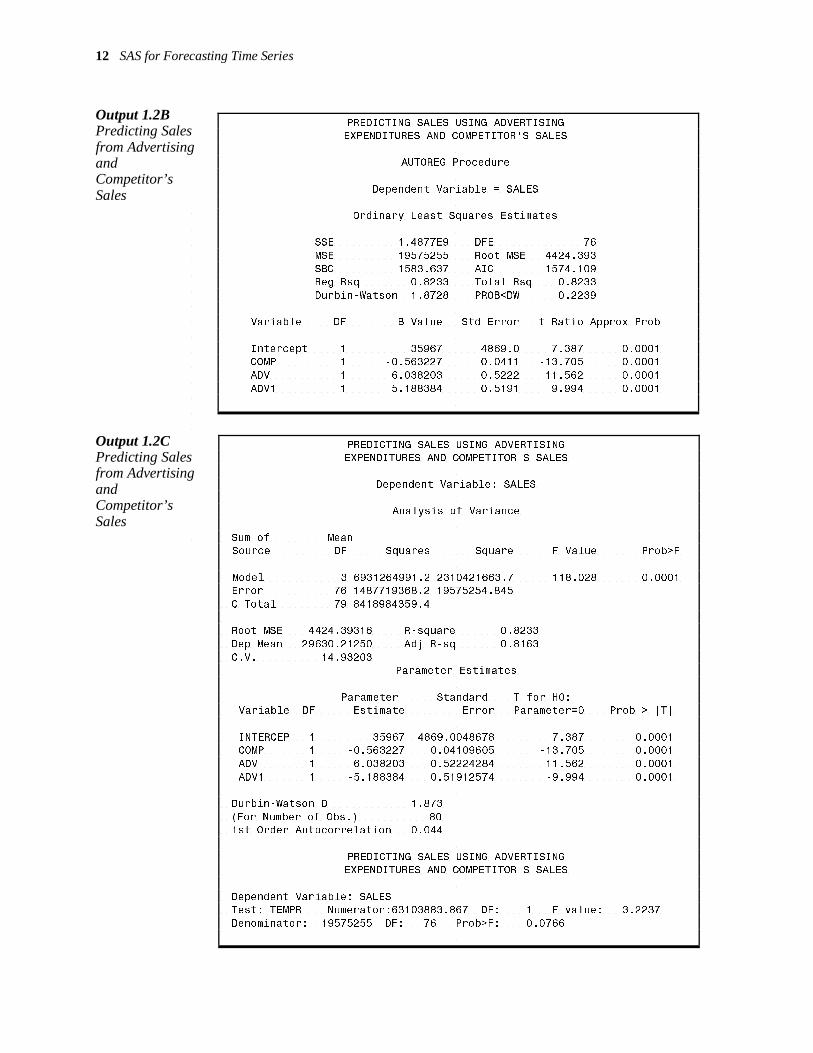
Now, in Output 1.2B, d =1.8728 is insignificant (p-value .2239 > .05). Note also the increase in R-square (the proportion of variation explained by the model) from 39% to 82%. What is the effect of an increase of $1 in advertising expenditure? It gives a sales increase estimated at $6.04 this period but a decrease of $5.18 next period. You wonder if the true coefficients on ADV and ADV1 are the same with opposite signs; that is, you wonder if these coefficients add to 0. If they do, then the increase we get this period from advertising is followed by a decrease of equal magnitude next
2
1ˆ ˆ ˆ ˆ/
t t t−
ρ = ε ε ε∑ ∑
2 2
1ˆ ˆ ˆd ( ) /
t t t−
= ε − ε ε∑ ∑
Chapter 1: Overview of Time Series 11
AUTOREG Procedure
Dependent Variable = SALES
Ordinary Least Squares Estimates
SSE 5.1646E9 DFE 77
MSE 67072080 Root MSE 8189.755
SBC 1678.821 AIC 1671.675 Reg Rsq 0.3866 Total Rsq 0.3866
Durbin-Watson 0.5427 PROB<DW 0.0001
Variable DF B Value Std Error t Ratio Approx Prob
Intercept 1 14466 8532.1 1.695 0.0940
ADV 1 6.560093 0.9641 6.804 0.0001
ADV1 1 -5.015231 0.9606 -5.221 0.0001
period. This means our advertising dollar simply shifts the timing of sales rather than increasing the level of sales. Having no autocorrelation evident, you fit the model in PROC REG asking for a test that the coefficients of ADV and ADV1 add to 0.
PROC REG DATA = SALES; MODEL SALES = ADV ADV1 COMP; TEMPR: TEST ADV+ADV1=0;
RUN;
Output 1.2C gives the results. Notice that the regression is exactly that given by PROC AUTOREG with no NLAG= specified. The p-value (.077>.05) is not small enough to reject the hypothesis that the coefficients are of equal magnitude, and thus it is possible that advertising just shifts the timing, a temporary effect. Note the label TEMPR on the test.
Note also that, although we may have information on our company’s plans to advertise, we would likely not know what our competitor’s sales will be in future months, so at best we would have to substitute estimates of these future values in forecasting our sales. It appears that an increase of $1.00 in our competitor’s sales is associated with a $0.56 decrease in our sales.
From Output 1.2C the forecasting equation is seen to be
PREDICTED SALES = 35967 – 0.563227COMP + 6.038203ADV – 5.188384ADV1
Output 1.2A Predicting Sales from Advertising
12 SAS for Forecasting Time Series
PREDICTING SALES USING ADVERTISING EXPENDITURES AND COMPETITOR'S SALES
AUTOREG Procedure
Dependent Variable = SALES
Ordinary Least Squares Estimates
SSE 1.4877E9 DFE 76
MSE 19575255 Root MSE 4424.393
SBC 1583.637 AIC 1574.109 Reg Rsq 0.8233 Total Rsq 0.8233
Durbin-Watson 1.8728 PROB<DW 0.2239
Variable DF B Value Std Error t Ratio Approx Prob
Intercept 1 35967 4869.0 7.387 0.0001 COMP 1 -0.563227 0.0411 -13.705 0.0001
ADV 1 6.038203 0.5222 11.562 0.0001
ADV1 1 -5.188384 0.5191 -9.994 0.0001
PREDICTING SALES USING ADVERTISING EXPENDITURES AND COMPETITOR'S SALES
Dependent Variable: SALES
Analysis of Variance
Sum of Mean Source DF Squares Square F Value Prob>F
Model 3 6931264991.2 2310421663.7 118.028 0.0001 Error 76 1487719368.2 19575254.845
C Total 79 8418984359.4
Root MSE 4424.39316 R-square 0.8233
Dep Mean 29630.21250 Adj R-sq 0.8163
C.V. 14.93203 Parameter Estimates
Parameter Standard T for H0: Variable DF Estimate Error Parameter=0 Prob > |T|
INTERCEP 1 35967 4869.0048678 7.387 0.0001 COMP 1 -0.563227 0.04109605 -13.705 0.0001
ADV 1 6.038203 0.52224284 11.562 0.0001
ADV1 1 -5.188384 0.51912574 -9.994 0.0001
Durbin-Watson D 1.873
(For Number of Obs.) 80 1st Order Autocorrelation 0.044
PREDICTING SALES USING ADVERTISING EXPENDITURES AND COMPETITOR'S SALES
Dependent Variable: SALES Test: TEMPR Numerator:63103883.867 DF: 1 F value: 3.2237
Denominator: 19575255 DF: 76 Prob>F: 0.0766
Output 1.2B Predicting Sales from Advertising and Competitor’s Sales
Output 1.2C Predicting Sales from Advertising and Competitor’s Sales
Chapter 1: Overview of Time Series 13
OBS DATE CHANGE S1 S2 S3 T1 T2
1 83Q1 . 1 0 0 1 1 2 83Q2 1678.41 0 1 0 2 4
3 83Q3 633.24 0 0 1 3 9
4 83Q4 662.35 0 0 0 4 16 5 84Q1 -1283.59 1 0 0 5 25
(More Output Lines)
47 94Q3 543.61 0 0 1 47 2209
48 94Q4 1526.95 0 0 0 48 2304
1.3.2 Highly Regular Seasonality Occasionally, a very regular seasonality occurs in a series, such as an average monthly temperature at a given location. In this case, you can model seasonality by computing means. Specifically, the mean of all the January observations estimates the seasonal level for January. Similar means are used for other months throughout the year. An alternative to computing the twelve means is to run a regression on monthly indicator variables. An indicator variable takes on values of 0 or 1. For the January indicator, the 1s occur only for observations made in January. You can compute an indicator variable for each month and regress Y
t on the twelve indicators with no intercept. You can also
regress Yt on a column of 1s and eleven of the indicator variables. The intercept now estimates the
level for the month associated with the omitted indicator, and the coefficient of any indicator column is added to the intercept to compute the seasonal level for that month.
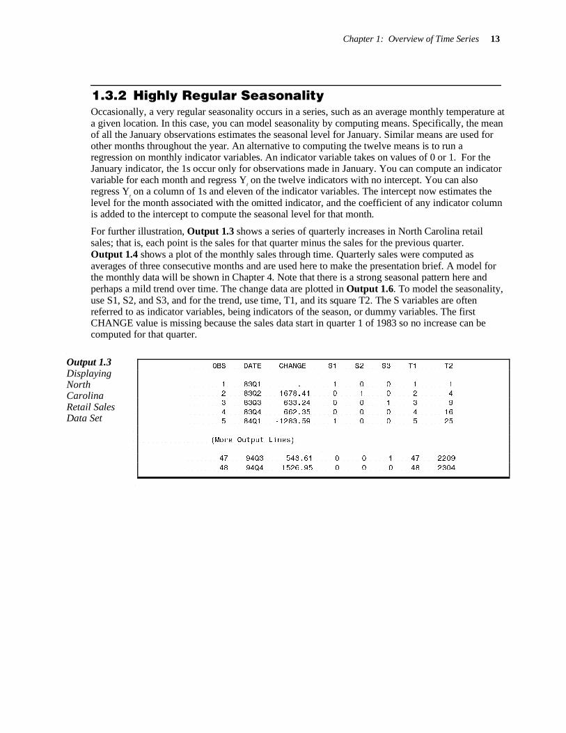
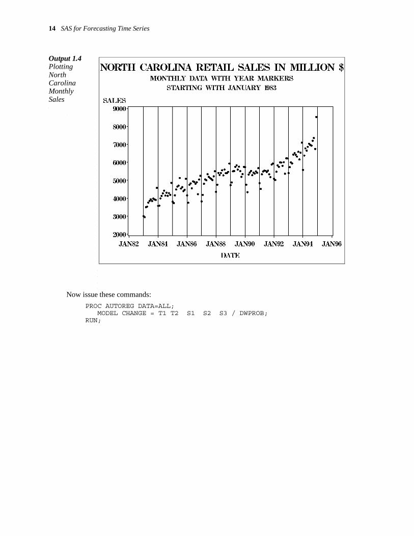
For further illustration, Output 1.3 shows a series of quarterly increases in North Carolina retail sales; that is, each point is the sales for that quarter minus the sales for the previous quarter. Output 1.4 shows a plot of the monthly sales through time. Quarterly sales were computed as averages of three consecutive months and are used here to make the presentation brief. A model for the monthly data will be shown in Chapter 4. Note that there is a strong seasonal pattern here and perhaps a mild trend over time. The change data are plotted in Output 1.6. To model the seasonality, use S1, S2, and S3, and for the trend, use time, T1, and its square T2. The S variables are often referred to as indicator variables, being indicators of the season, or dummy variables. The first CHANGE value is missing because the sales data start in quarter 1 of 1983 so no increase can be computed for that quarter.
Output 1.3 Displaying North Carolina Retail Sales Data Set
14 SAS for Forecasting Time Series
Output 1.4 Plotting North Carolina Monthly Sales
Now issue these commands:
PROC AUTOREG DATA=ALL; MODEL CHANGE = T1 T2 S1 S2 S3 / DWPROB;
RUN;
Chapter 1: Overview of Time Series 15
AUTOREG Procedure
Dependent Variable = CHANGE
Ordinary Least Squares Estimates
SSE 5290128 DFE 41
MSE 129027.5 Root MSE 359.204
SBC 703.1478 AIC 692.0469 Reg Rsq 0.9221 Total Rsq 0.9221
Durbin-Watson 2.3770 PROB<DW 0.8608
Variable DF B Value Std Error t Ratio Approx Prob
Intercept 1 679.427278 200.1 3.395 0.0015
T1 1 -44.992888 16.4428 -2.736 0.0091 T2 1 0.991520 0.3196 3.102 0.0035
S1 1 -1725.832501 150.3 -11.480 0.0001
S2 1 1503.717849 146.8 10.240 0.0001 S3 1 -221.287056 146.7 -1.508 0.1391
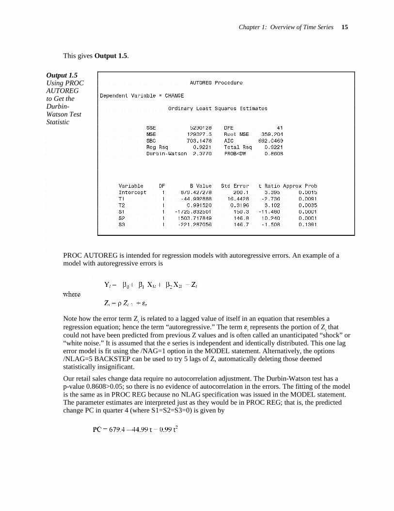
This gives Output 1.5.
Output 1.5 Using PROC AUTOREG to Get the Durbin-Watson Test Statistic
PROC AUTOREG is intended for regression models with autoregressive errors. An example of a model with autoregressive errors is
Yt = 0
β + 1β X1t +
2β X2t + Zt
where
Zt = ρ Zt–1 + gt
Note how the error term Zt is related to a lagged value of itself in an equation that resembles a
regression equation; hence the term “autoregressive.” The term gt represents the portion of Z
t that
could not have been predicted from previous Z values and is often called an unanticipated “shock” or “white noise.” It is assumed that the e series is independent and identically distributed. This one lag error model is fit using the /NAG=1 option in the MODEL statement. Alternatively, the options /NLAG=5 BACKSTEP can be used to try 5 lags of Z, automatically deleting those deemed statistically insignificant.
Our retail sales change data require no autocorrelation adjustment. The Durbin-Watson test has a p-value 0.8608>0.05; so there is no evidence of autocorrelation in the errors. The fitting of the model is the same as in PROC REG because no NLAG specification was issued in the MODEL statement. The parameter estimates are interpreted just as they would be in PROC REG; that is, the predicted change PC in quarter 4 (where S1=S2=S3=0) is given by
PC = 679.4 – 44.99 t + 0.99 t2
16 SAS for Forecasting Time Series
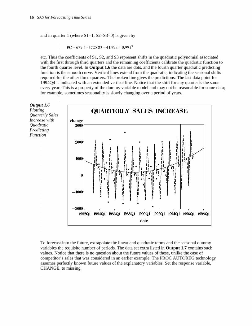
and in quarter 1 (where S1=1, S2=S3=0) is given by
PC = 679.4 –1725.83 – 44.99 t + 0.99 t2
etc. Thus the coefficients of S1, S2, and S3 represent shifts in the quadratic polynomial associated with the first through third quarters and the remaining coefficients calibrate the quadratic function to the fourth quarter level. In Output 1.6 the data are dots, and the fourth quarter quadratic predicting function is the smooth curve. Vertical lines extend from the quadratic, indicating the seasonal shifts required for the other three quarters. The broken line gives the predictions. The last data point for 1994Q4 is indicated with an extended vertical line. Notice that the shift for any quarter is the same every year. This is a property of the dummy variable model and may not be reasonable for some data; for example, sometimes seasonality is slowly changing over a period of years.
Output 1.6 Plotting Quarterly Sales Increase with Quadratic Predicting Function
To forecast into the future, extrapolate the linear and quadratic terms and the seasonal dummy variables the requisite number of periods. The data set extra listed in Output 1.7 contains such values. Notice that there is no question about the future values of these, unlike the case of competitor’s sales that was considered in an earlier example. The PROC AUTOREG technology assumes perfectly known future values of the explanatory variables. Set the response variable, CHANGE, to missing.
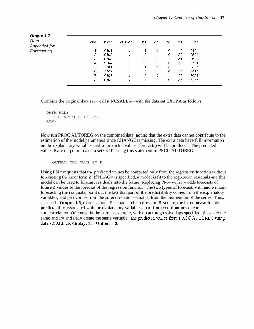
Chapter 1: Overview of Time Series 17
OBS DATE CHANGE S1 S2 S3 T1 T2
1 95Q1 . 1 0 0 49 2401 2 95Q2 . 0 1 0 50 2500
3 95Q3 . 0 0 1 51 2601
4 95Q4 . 0 0 0 52 2704 5 96Q1 . 1 0 0 53 2809
6 96Q2 . 0 1 0 54 2916
7 96Q3 . 0 0 1 55 3025
8 96Q4 . 0 0 0 56 3136
Output 1.7 Data Appended for Forecasting
Combine the original data set—call it NCSALES—with the data set EXTRA as follows:
DATA ALL; SET NCSALES EXTRA; RUN;
Now run PROC AUTOREG on the combined data, noting that the extra data cannot contribute to the estimation of the model parameters since CHANGE is missing. The extra data have full information on the explanatory variables and so predicted values (forecasts) will be produced. The predicted values P are output into a data set OUT1 using this statement in PROC AUTOREG:
OUTPUT OUT=OUT1 PM=P;
Using PM= requests that the predicted values be computed only from the regression function without forecasting the error term Z. If NLAG= is specified, a model is fit to the regression residuals and this model can be used to forecast residuals into the future. Replacing PM= with P= adds forecasts of future Z values to the forecast of the regression function. The two types of forecast, with and without forecasting the residuals, point out the fact that part of the predictability comes from the explanatory variables, and part comes from the autocorrelation—that is, from the momentum of the series. Thus, as seen in Output 1.5, there is a total R-square and a regression R-square, the latter measuring the predictability associated with the explanatory variables apart from contributions due to autocorrelation. Of course in the current example, with no autoregressive lags specified, these are the same and P= and PM= create the same variable. The predicted values from PROC AUTOREG using data set ALL are displayed in Output 1.8.
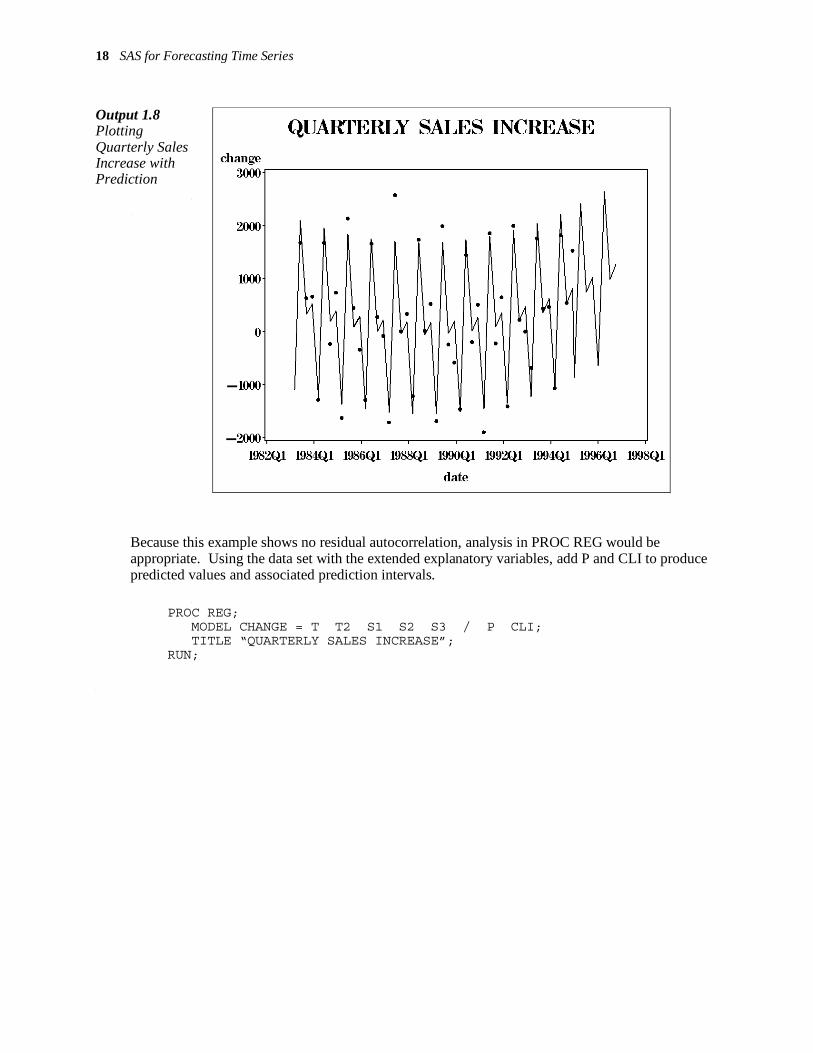
18 SAS for Forecasting Time Series
Output 1.8 Plotting Quarterly Sales Increase with Prediction
Because this example shows no residual autocorrelation, analysis in PROC REG would be appropriate. Using the data set with the extended explanatory variables, add P and CLI to produce predicted values and associated prediction intervals.
PROC REG; MODEL CHANGE = T T2 S1 S2 S3 / P CLI; TITLE “QUARTERLY SALES INCREASE”;
RUN;
Chapter 1: Overview of Time Series 19
QUARTERLY SALES INCREASE
Dependent Variable: CHANGE
Analysis of Variance
Sum of Mean
Source DF Squares Square F Value Prob>F
Model 5 62618900.984 12523780.197 97.063 0.0001
Error 41 5290127.6025 129027.5025
C Total 46 67909028.586
Root MSE 359.20398 R-square 0.9221
Dep Mean 280.25532 Adj R-sq 0.9126 C.V. 128.17026
Parameter Estimates
Parameter Standard T for H0:
Variable DF Estimate Error Parameter=0 Prob > |T|
INTERCEP 1 679.427278 200.12467417 3.395 0.0015
T1 1 -44.992888 16.44278429 -2.736 0.0091 T2 1 0.991520 0.31962710 3.102 0.0035
S1 1 -1725.832501 150.33120614 -11.480 0.0001
S2 1 1503.717849 146.84832151 10.240 0.0001 S3 1 -221.287056 146.69576462 -1.508 0.1391
Quarterly Sales Increase
Dep Var Predict Std Err Lower95% Upper95%
Obs CHANGE Value Predict Predict Predict Residual
1 . -1090.4 195.006 -1915.8 -265.0 .
2 1678.4 2097.1 172.102 1292.7 2901.5 -418.7 3 633.2 332.1 163.658 -465.1 1129.3 301.2
4 662.4 515.3 156.028 -275.6 1306.2 147.0
5 -1283.6 -1246.6 153.619 -2035.6 -457.6 -37.0083
(more output lines)
49 . -870.4 195.006 -1695.9 -44.9848 .
50 . 2412.3 200.125 1581.9 3242.7 .
51 . 742.4 211.967 -99.8696 1584.8 . 52 . 1020.9 224.417 165.5 1876.2 .
53 . -645.8 251.473 -1531.4 239.7 .
54 . 2644.8 259.408 1750.0 3539.6 . 55 . 982.9 274.992 69.2774 1896.5 .
56 . 1269.2 291.006 335.6 2202.8 .
Sum of Residuals 0
Sum of Squared Residuals 5290127.6025
Predicted Resid SS (Press) 7067795.5909
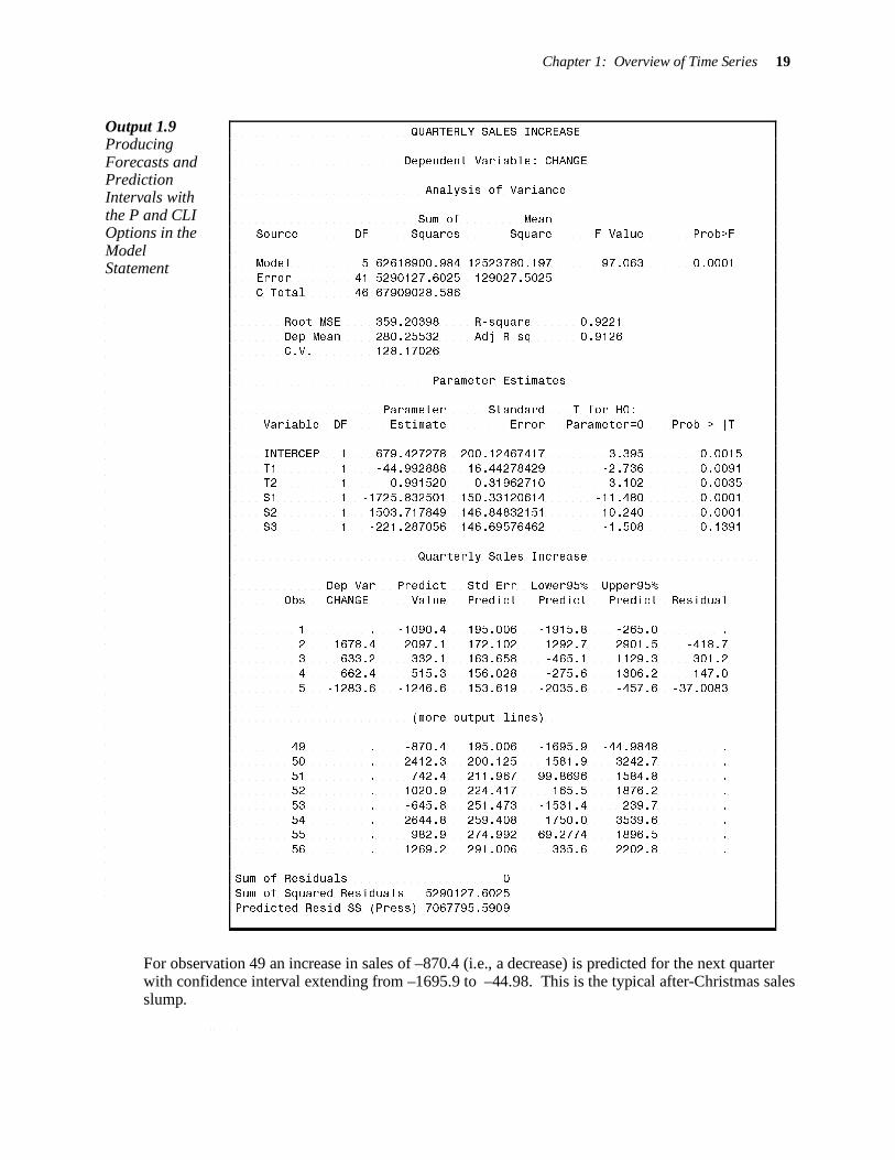
Output 1.9 Producing Forecasts and Prediction Intervals with the P and CLI Options in the Model Statement
For observation 49 an increase in sales of –870.4 (i.e., a decrease) is predicted for the next quarter with confidence interval extending from –1695.9 to –44.98. This is the typical after-Christmas sales slump.
20 SAS for Forecasting Time Series
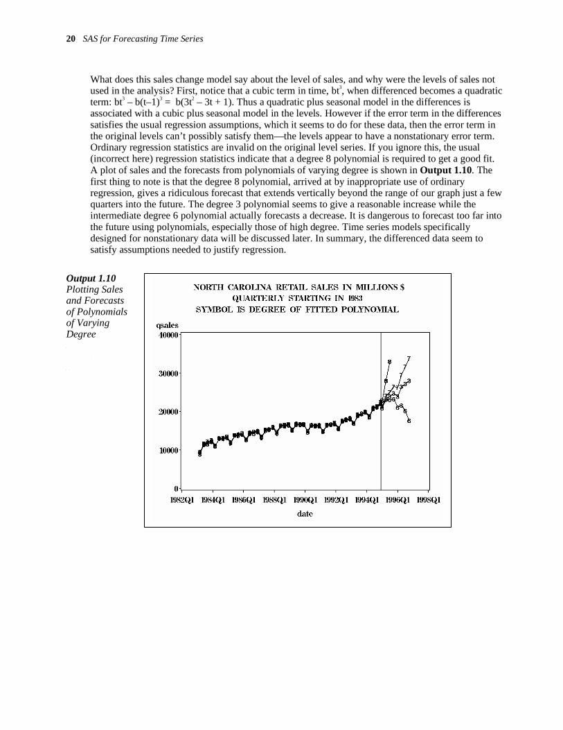
What does this sales change model say about the level of sales, and why were the levels of sales not used in the analysis? First, notice that a cubic term in time, bt3, when differenced becomes a quadratic term: bt3 – b(t–1)3 = b(3t2 – 3t + 1). Thus a quadratic plus seasonal model in the differences is associated with a cubic plus seasonal model in the levels. However if the error term in the differences satisfies the usual regression assumptions, which it seems to do for these data, then the error term in the original levels can’t possibly satisfy them—the levels appear to have a nonstationary error term. Ordinary regression statistics are invalid on the original level series. If you ignore this, the usual (incorrect here) regression statistics indicate that a degree 8 polynomial is required to get a good fit. A plot of sales and the forecasts from polynomials of varying degree is shown in Output 1.10. The first thing to note is that the degree 8 polynomial, arrived at by inappropriate use of ordinary regression, gives a ridiculous forecast that extends vertically beyond the range of our graph just a few quarters into the future. The degree 3 polynomial seems to give a reasonable increase while the intermediate degree 6 polynomial actually forecasts a decrease. It is dangerous to forecast too far into the future using polynomials, especially those of high degree. Time series models specifically designed for nonstationary data will be discussed later. In summary, the differenced data seem to satisfy assumptions needed to justify regression.
Output 1.10 Plotting Sales and Forecasts of Polynomials of Varying Degree
Chapter 1: Overview of Time Series 21
1.3.3 Regression with Transformed Data Often, you analyze some transformed version of the data rather than the original data. The logarithmic transformation is probably the most common and is the only transformation discussed in this book. Box and Cox (1964) suggest a family of transformations and a method of using the data to select one of them. This is discussed in the time series context in Box and Jenkins (1976, 1994).
Consider the following model:
( )X
0 1Y t
t tε= β β
Taking logarithms on both sides, you obtain
( ) ( ) ( ) ( )0 1log Y log log X log
t t tε= β + β +
Now if
( )logt t
εη =
and if tη satisfies the standard regression assumptions, the regression of log(Y
t) on 1 and X
t
produces the best estimates of log(0β ) and log(
1β ).
As before, if the data consist of (X1, Y
1), (X
2, Y
2), ..., (X
n, Y
n), you can append future known values
Xn+1
, Xn+2
, ..., Xn+s
to the data if they are available. Set Yn+1
through Yn+s
to missing values (.). Now use the MODEL statement in PROC REG:
MODEL LY=X / P CLI; where
LY=LOG(Y);
is specified in the DATA step. This produces predictions of future LY values and prediction limits for them. If, for example, you obtain an interval
−1.13 < log(Yn+s
) < 2.7
you can compute
exp(−1.13) = .323
and
exp(2.7) = 14.88
to conclude
.323 < Yn+s
< 14.88
Note that the original prediction interval had to be computed on the log scale, the only scale on which you can justify a t distribution or normal distribution.
When should you use logarithms? A quick check is to plot Y against X. When
( )X
0 1Y t
t tε= β β
the overall shape of the plot resembles that of
( )X
0 1Y = β β
22 SAS for Forecasting Time Series
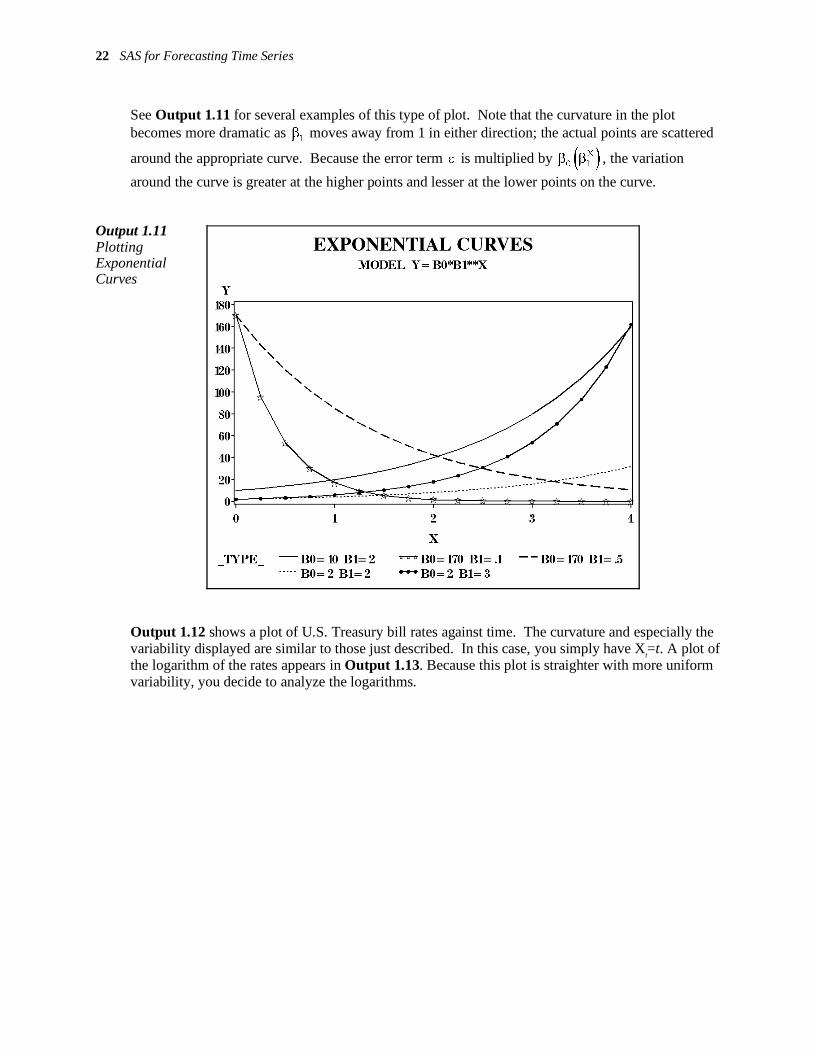
See Output 1.11 for several examples of this type of plot. Note that the curvature in the plot becomes more dramatic as
1β moves away from 1 in either direction; the actual points are scattered
around the appropriate curve. Because the error term ε is multiplied by ( )X
0 1β β , the variation
around the curve is greater at the higher points and lesser at the lower points on the curve.
Output 1.11 Plotting Exponential Curves
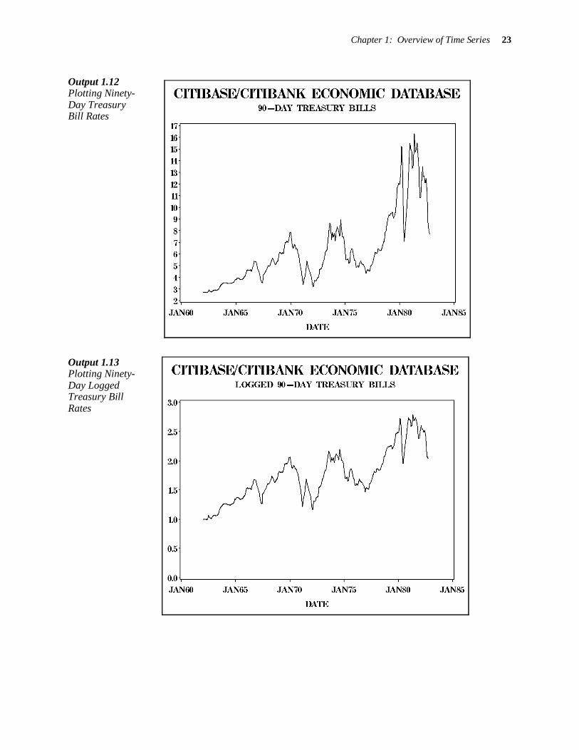
Output 1.12 shows a plot of U.S. Treasury bill rates against time. The curvature and especially the variability displayed are similar to those just described. In this case, you simply have X
t=t. A plot of
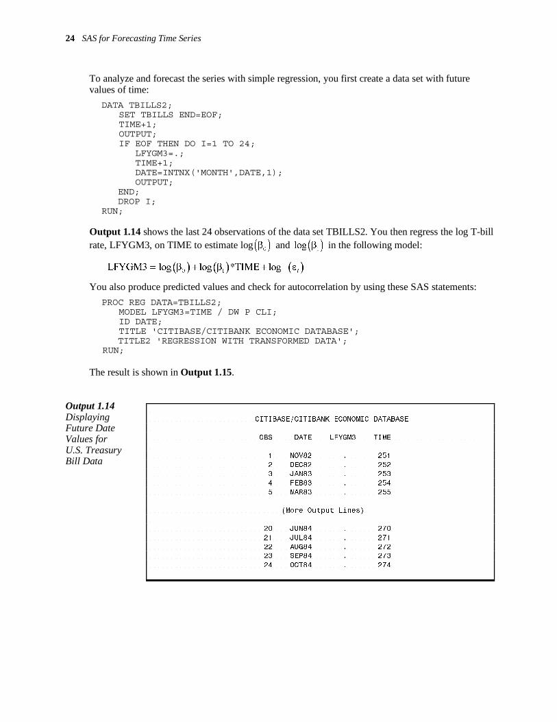
the logarithm of the rates appears in Output 1.13. Because this plot is straighter with more uniform variability, you decide to analyze the logarithms.
Chapter 1: Overview of Time Series 23
Output 1.12 Plotting Ninety-Day Treasury Bill Rates
Output 1.13 Plotting Ninety-Day Logged Treasury Bill Rates
24 SAS for Forecasting Time Series
CITIBASE/CITIBANK ECONOMIC DATABASE
OBS DATE LFYGM3 TIME
1 NOV82 . 251
2 DEC82 . 252 3 JAN83 . 253
4 FEB83 . 254
5 MAR83 . 255
(More Output Lines)
20 JUN84 . 270
21 JUL84 . 271
22 AUG84 . 272 23 SEP84 . 273
24 OCT84 . 274
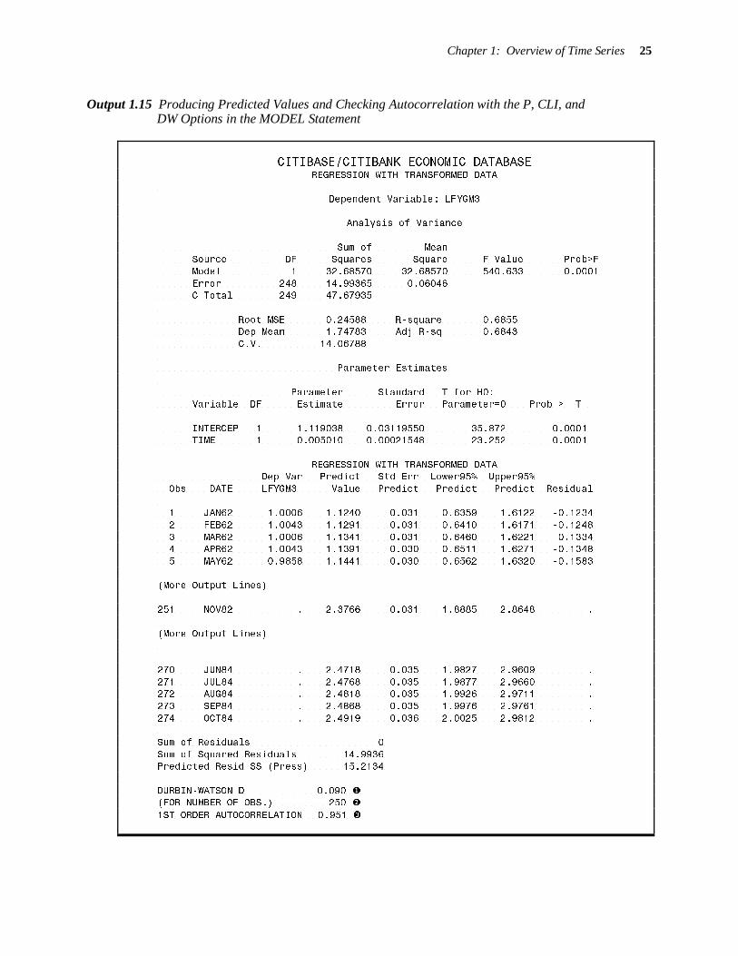
To analyze and forecast the series with simple regression, you first create a data set with future values of time:
DATA TBILLS2; SET TBILLS END=EOF; TIME+1; OUTPUT; IF EOF THEN DO I=1 TO 24; LFYGM3=.; TIME+1; DATE=INTNX('MONTH',DATE,1); OUTPUT;
END; DROP I; RUN;
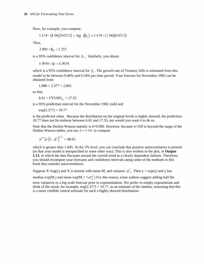
Output 1.14 shows the last 24 observations of the data set TBILLS2. You then regress the log T-bill rate, LFYGM3, on TIME to estimate log ( )0
β and ( )1log β in the following model:
( ) ( ) ( )0 1LFYGM3 log log *TIME log
t= β + β + ε
You also produce predicted values and check for autocorrelation by using these SAS statements:
PROC REG DATA=TBILLS2; MODEL LFYGM3=TIME / DW P CLI; ID DATE; TITLE 'CITIBASE/CITIBANK ECONOMIC DATABASE'; TITLE2 'REGRESSION WITH TRANSFORMED DATA';
RUN;
The result is shown in Output 1.15.
Output 1.14 Displaying Future Date Values for U.S. Treasury Bill Data
Chapter 1: Overview of Time Series 25
Output 1.15 Producing Predicted Values and Checking Autocorrelation with the P, CLI, and DW Options in the MODEL Statement
CITIBASE/CITIBANK ECONOMIC DATABASE REGRESSION WITH TRANSFORMED DATA
Dependent Variable: LFYGM3
Analysis of Variance
Sum of Mean Source DF Squares Square F Value Prob>F
Model 1 32.68570 32.68570 540.633 0.0001
Error 248 14.99365 0.06046 C Total 249 47.67935
Root MSE 0.24588 R-square 0.6855 Dep Mean 1.74783 Adj R-sq 0.6843
C.V. 14.06788
Parameter Estimates
Parameter Standard T for H0: Variable DF Estimate Error Parameter=0 Prob > |T|
INTERCEP 1 1.119038 0.03119550 35.872 0.0001 TIME 1 0.005010 0.00021548 23.252 0.0001
REGRESSION WITH TRANSFORMED DATA Dep Var Predict Std Err Lower95% Upper95%
Obs DATE LFYGM3 Value Predict Predict Predict Residual
1 JAN62 1.0006 1.1240 0.031 0.6359 1.6122 -0.1234
2 FEB62 1.0043 1.1291 0.031 0.6410 1.6171 -0.1248
3 MAR62 1.0006 1.1341 0.031 0.6460 1.6221 -0.1334 4 APR62 1.0043 1.1391 0.030 0.6511 1.6271 -0.1348
5 MAY62 0.9858 1.1441 0.030 0.6562 1.6320 -0.1583
(More Output Lines)
251 NOV82 . 2.3766 0.031 1.8885 2.8648 .
(More Output Lines)
270 JUN84 . 2.4718 0.035 1.9827 2.9609 .
271 JUL84 . 2.4768 0.035 1.9877 2.9660 . 272 AUG84 . 2.4818 0.035 1.9926 2.9711 .
273 SEP84 . 2.4868 0.035 1.9976 2.9761 .
274 OCT84 . 2.4919 0.036 2.0025 2.9812 .
Sum of Residuals 0
Sum of Squared Residuals 14.9936 Predicted Resid SS (Press) 15.2134
DURBIN-WATSON D 0.090 � (FOR NUMBER OF OBS.) 250 �
1ST ORDER AUTOCORRELATION 0.951 �
26 SAS for Forecasting Time Series
Now, for example, you compute:
( ) ( ) ( ) ( ) ( )01.119 1.96 0.0312 log 1.119 1.96 0.0312− < β < +
Thus,
02.880 3.255< β <
is a 95% confidence interval for 0
β . Similarly, you obtain
11.0046 1.0054< β <
which is a 95% confidence interval for 1β . The growth rate of Treasury bills is estimated from this
model to be between 0.46% and 0.54% per time period. Your forecast for November 1982 can be obtained from
1.888 < 2.377 < 2.865
so that
6.61 < FYGM3251
< 17.55
is a 95% prediction interval for the November 1982 yield and
exp(2.377) = 10.77
is the predicted value. Because the distribution on the original levels is highly skewed, the prediction 10.77 does not lie midway between 6.61 and 17.55, nor would you want it to do so.
Note that the Durbin-Watson statistic is d=0.090. However, because n=250 is beyond the range of the Durbin-Watson tables, you use 951.0ˆ =ρ to compute
( )1/ 2
1/ 2 2ˆ ˆn / 1ρ −ρ = 48.63
which is greater than 1.645. At the 5% level, you can conclude that positive autocorrelation is present (or that your model is misspecified in some other way). This is also evident in the plot, in Output 1.13, in which the data fluctuate around the overall trend in a clearly dependent fashion. Therefore, you should recompute your forecasts and confidence intervals using some of the methods in this book that consider autocorrelation.
Suppose X=log(y) and X is normal with mean Mx and variance 2
xσ . Then y = exp(x) and y has
median exp(Mx) and mean exp(M
x+ ½ 2
xσ ) For this reason, some authors suggest adding half the
error variances to a log scale forecast prior to exponentiation. We prefer to simply exponentiate and think of the result, for example, exp(2.377) = 10.77, as an estimate of the median, reasoning that this is a more credible central estimate for such a highly skewed distribution.