1 Overview of Labor Markets and Labor De- mand Labor Economics (Undergraduate), Review Problems 1 1 Overview of Labor Markets and Labor De-mand Question 1: Show in a labor supply and

Wiswall, Labor Economics (Undergraduate), Review Problems 1

1 Overview of Labor Markets and Labor De-

mand

Question 1: Show in a labor supply and demand graph the effect of each of

these changes. Indicate whether the equilibrium wage rate and the equilib-

rium number of hours worked increases or decreases. Draw a separate graph

for each. Note: each of these involves a shift of the demand or supply curve

for labor.

a) Increased supply of labor.

b) Decreased demand for labor.

c) A minimum wage law is imposed above the equilibrium wage.

d) A minimum wage law is imposed below the equilibrium wage.

Question 2: Provide one realistic example for each of the following. Note:

each of these involves a shift of the demand or supply curve for labor.

a) Increased supply of labor.

b) Decreased supply of labor.

c) Increased demand for labor.

d) Decreased demand for labor.

Question 3: Using the labor supply and demand model, provide an explana-

tion for these observed change in the equilibrium wage rate and equilibrium

hours worked.

a) Higher wage rate and more hours worked.


b) Lower wage rate and fewer hours worked.

c) Higher wage rate and fewer hours worked.

d) Lower wage rate and more hour worked.

Question 4: A survey asked how much a respondent worked in the past

week and how much they were paid per hour. 5 people responded to the

survey. Here is the collected data:

Respondent 1, 40 hours, $10 per hour





Calculate the following:

a) Average hourly wage. 11 (for those who work)

b) Average hours worked. 37.5 (for those who work)

c) Unemployment rate (assuming each of the respondents is in the labor

force). 1/5

d) Unemployment rate (assuming everyone but Respondent 4 is in the

labor force). 0

e) Labor force participation rate (assuming everyone but Respondent 4

is in the labor force). 4/5

Answer the following:


f) What additional information would we need to know to determine

whether Respondent 4 is in the labor force?

g) Provide at least two independent reasons why these people are working

different number of hours.

h) Provide at least two independent reasons why these people are being

paid different wage rates.

Question 5

a) Draw the following labor supply and demand curves in one graph.

Label each axis, each curve, the equilibrium labor hours employed (h∗), and

the equilibrium wage rate (w∗).

Labor Demand Curve:

h = 4 − 1

2w

Labor Supply Curve:

h = −1 +1

2w

b) Calculate the equilibrium wage rate (w∗) and the equilibrium number

of labor hours employed (h∗) in this market.

Answer:

w∗ = 5, h∗ = 32

c) In your graph, draw a minimum wage at w′ = $7. In the graph, indicate

the new equilibrium number of labor hours employed (h′).


d) Under the minimum wage of w′ = $7, calculate the new equilibrium

amount of labor employed (h′) and the new equilibrium wage rate (w′).

Answer:

w′ = 7, h′ = 12

e) Under the minimum wage of w′ = $10, calculate the new equilibrium

amount of labor employed (h′) and the new equilibrium wage rate (w′). w′ =

$10, h′ = −1 or h′ = 0 (the firm hires no labor at this wage rate).

Question 6

Assume the production function is

q = f(h, k) = 4h1/2 + 2k1/2

a) Calculate the following (as functions of input prices, output price, labor

hours, capital hours, etc.):

i) marginal product of labor (MPh) 2h−1/2

ii) marginal product of capital (MPk) k−1/2

iii) marginal revenue product of labor (MRPh) p2h−1/2

iv) marginal revenue product of capital (MRPk) pk−1/2

v) marginal rate of technical substitution (MRTS) 2k1/2

h1/2

b) Write the profit maximization problem for the firm.

c) Calculate the profit maximizing level of labor demand (h∗) as a function

of the output price p and input prices (w and r).


Answer:

h∗ = 4 p2

w2

d) Calculate the profit maximizing level of capital demand (k∗) as a func-

tion of output prices p and input prices (w and r). k∗ = p2

r2

e) Assume p = 2, w = 12, and r = 3. Calculate the profit maximizing

level of labor demand (h∗), capital demand (k∗), and output (q∗). How much

profit is the firm making?

Answer:

I’ll just do one: h∗ = 4 22

( 12)2

= 4 ∗ 4 ∗ 4 = 64.

f) If w increases to w = 3 (and p and r stay at p = 2 and r = 3), what

is the new profit maximizing level of labor demand, capital demand, and

output? How much profit is the firm making?

Answer:

I’ll just do one: h∗ = 422

32 = 4 ∗ 4 ∗ 19

= 169

g) If p increases to p = 4 (and w and r stay at w = 1/2 and r = 3),

what is the new profit maximizing level of labor demand, capital demand,

and output? How much profit is the firm making?

Answer:

h∗ = 4 42

1/22 = 4 ∗ 16 ∗ 4 = 256


h) Calculate the labor demand elasticity with respect to wages (ε). (Note:

your answer should be a function of h∗, w, p, and r).

Answer:

ε = −8 ∗ p2 ∗ w−2 ∗ 1h∗

i) What is the labor demand elasticity at w = 3, r = 3, and p = 2? (Note:

your answer should be a number, not a function.)

Answer:

ε = −8 ∗ 22 ∗ 3−2 ∗ 9/16 = −2

j) What is the labor demand elasticity at w = 1/2, r = 3, and p = 4?

(Note: your answer should be a number, not a function.)

Answer:

ε = −8 ∗ 42 ∗ 1/2−2 ∗ 1/256 = −8 ∗ 16 ∗ 4 ∗ 1/256 = −2

Question 7

Assume the production function is

q = f(h, k) = h1/2

a) Calculate the following (as functions of input prices, output price, labor

hours, capital hours, etc.):

i) marginal product of labor (MPh) 1/2 ∗ h−1/2


ii) marginal product of capital (MPk) 0

iii) marginal revenue product of labor (MRPh) p ∗ 1/2 ∗ h−1/2

iv) marginal revenue product of capital (MRPk) 0

b) Write the profit maximization problem for the firm.

c) Calculate the profit maximizing level of labor demand (h∗) as a function

of the output price p and input prices (w and r).

Answer:

h∗ = p2

4w2

d) Calculate the profit maximizing level of capital demand (k∗) as a func-

tion of output prices p and input prices (w and r).

e) Assume p = 2, w = 1/2, and r = 3. Calculate the profit maximizing

level of labor demand (h∗), capital demand (k∗), and output (q∗). How much

profit is the firm making?

Answer:

h∗ = 22

41/22 = 4 ∗ 1 = 4

f) If w increases to w = 3 (and p and r stay at p = 2 and r = 3), what

is the new profit maximizing level of labor demand, capital demand, and

output? How much profit is the firm making?

Answer:

h∗ = 22

4∗32 = 4/36 = 1/9


g) If p increases to p = 4 (and w and r stay at w = 1/2 and r = 3),

what is the new profit maximizing level of labor demand, capital demand,

and output? How much profit is the firm making?

h) Calculate the labor demand elasticity with respect to wages (ε). (Note:

your answer should be a function of h∗, w, and p).

Answer:

ε = −12∗ p2 ∗ w−2 ∗ 1

h∗

i) What is the labor demand elasticity at w = 3, r = 3, and p = 2? (Note:

your answer should be a number, not a function.)

Answer:

ε = −12∗ 22 ∗ 3−2 ∗ 9 = −2

j) What is the labor demand elasticity at w = 1/2, r = 3, and p = 4?

(Note: your answer should be a number, not a function.)


2 Labor Supply

Question 1

Assume the utility function has this form

U(c, l) = 2 c l1/2.

The individual has an endowment of V in non-labor income and T hours

to either work (h) or use for leisure (l).

a) Calculate the following as functions:

i) Marginal utility of leisure (MUl). cl−1/2

ii) Marginal utility of consumption (MUc). 2l1/2

iii) Marginal rate of substitution (MRS). c2l

iv) Total expenditure on consumer goods. pc

v) Total income. V + wh or V + w(T − l)

b) Write the budget constraint for this problem.

Answer:

V + wh = pc

c) Write the individual’s utility maximization problem.

Answer:


maxc,l

2cl1/2 s.t. V + wh = pc

d) Write the tangency condition for this problem.

Answer:

c2l

= wp

e) Derive the utility maximizing choices of leisure hours l∗, labor hours h∗,

and consumption of consumer goods c∗. Your answers should be functions.

Answer:

l∗ =V + wT

3w

h∗ = T − V + wT

3w

c∗ = V/p + w/p(T − V + wT

3w)

f) Show that the budget constraint is satisfied given these choices.

Answer:


V + wh∗ = pc∗

V + w(T − V + wT

3w) = p[V/p + w/p(T − V + wT

3w)]

V + w(T − V + wT

3w) = V + w(T − V + wT

3w)

g) Show that the time constraint is satisfied given these choices (T =

l∗ + h∗).

Answer:

l∗ + h∗ = T

T − V + wT

3w+

V + wT

3w= T

h) Assume the T = 16, p = 2, w = 1, and V = 5. What are the utility

maximizing choices of leisure hours l∗, labor hours h∗, and consumption of

consumer goods c∗? What is the total utility the individual is receiving given

these choices? Your answers should be numbers.


Answer:

l∗ = 5+1∗163∗1 = 21

3= 7

h∗ = 16 − 7 = 9

c∗ = 52

+ 12∗ 9 = 7

U = 2 ∗ 7 ∗ 71/2 = 14 ∗ 71/2

i) Show that the tangency condition (MRS = wp) is satisfied given your

answers in h).

Answer:

72∗7 = 1

2

j) Show that your answers in h) satisfy the budget constraint and the

time constraint.

Answer:

pc∗ = V + wh∗, 2 ∗ 7 = 5 + 1 ∗ 9

T = l∗ + h∗, 16 = 7 + 9

k) Calculate the elasticity of labor supply with respect to wages (γ). Your

answer should be a function.

Answer:

First, re-write h∗

h∗ = T − V + wT

3w= T − V

3w− T

3


∂h∗

∂w=

1

3∗ V ∗ w−2

γ =1

3∗ V ∗ w−2 ∗ w

h∗ =V

3w∗ 1

h∗

l) Assume the T = 16, p = 2, w = 1, and V = 5. Calculate γ at these

values. Your answer should be a number.

Answer:

γ =5

3∗ 1

9=

5

27

m)

i) Assume that w increases to w = 2 and everything else stays at the

initial values (T = 16, p = 2, w = 2, and V = 5). What are the utility




Answer:

l∗ =V + wT

3w


l∗ =5 + 2 ∗ 16

3 ∗ 2=

37

6

ii) Has labor supply increased or decreased after this increase in the wage

rate? Does this indicate that the substitution or income effect is stronger?

n) Show that the tangency condition (MRS = wp) is satisfied given your

answers in m). Also, show that your answers in m) satisfy the budget con-

straint and the time constraint.

o) Calculate γ at the new wage rate in m). Your answer should be a

number.

p)

i) Assume V increases to V = 8 and everything else stays at the initial

values (T = 16, p = 2, w = 1, and V = 8). What are the utility maximizing

choices of leisure hours l∗, labor hours h∗, and consumption of consumer

goods c∗? What is the total utility the individual is receiving given these

choices? Your answers should be numbers.

Answer:

l∗ =8 + 1 ∗ 16

3 ∗ 1= 8


ii) Has labor supply increased or decreased after this increase in non-labor

income? Does this indicate leisure is a normal good?

q) Show that the tangency condition (MRS = wp) is satisfied given your

answers in p). Also, show that your answers in p) satisfy the budget con-

straint and the time constraint.

r) Calculate γ at the new level of V in p). Your answer should be a

number.

Question 2

Assume the same utility function as in Question 1.

a) Assume T = 16, p = 2, w = 1. Find the minimum level of non-labor

income V at which this individuals will not work (l∗ = T ).

Answer:

From above,

l∗ =V + wT

3w

Set l∗ = T , substitute, and solve for V :

T =V + wT

3w

3wT = V + wT


V = 2wT

Substitute prices and T ,

V = 2 ∗ 1 ∗ 16 = 32

Check to make sure that at this V the individual never works.

l∗ =32 + 1 ∗ 16

3 ∗ 1=

48

3= 16 = T

b) Assume the T = 16, p = 2, w = 1. Find the maximum level of

non-labor income V at which this individual will always work (l∗ = 0).

c) Assume that w increases: T = 16, p = 2, w = 2. Find the minimum

level of non-labor income V at which this individual will not work (l∗ = T ).

Answer:

V = 2wT = 2 ∗ 2 ∗ 16 = 64

d) Assume that w increases: T = 16, p = 2, w = 2. Find the maximum

level of non-labor income V at which this individual will always work (l∗ = 0).

e) Explain (in words) why changes in the wage rate affect your answers.


In your discussion, reference the distinction between income and substitution

effects.

f) Assume T = 16, p = 2, V = 8. Find the reservation wage for this

individual.

Answer:

The reservation wage the level of w where the person is just indifferent

between working and not (l∗ = T ).

l∗ =V + wT

3w

T =V + wT

3w

3wT = V + wT

2wT = V

w =V

2T=

8

2 ∗ 16=

1

4

Confirm that at w = 1/4, the individual does not work:


l∗ =8 + 1/4 ∗ 16

3 ∗ 1/4=

12

3/4= 16

At a w higher than the reservation wage, the individual does work. Try,

w = 1/2.

l∗ =8 + 1/2 ∗ 16

3 ∗ 1/2=

16

3/2= 32/3 < 16

g) Assume non-labor income decreases: T = 16, p = 2, V = 4. Find

the reservation wage for this individual. Briefly explain why this change in

non-labor income changed the reservation wage level.

h) Assume non-labor income increases: T = 16, p = 2, V = 10. Find

the reservation wage for this individual. Briefly explain why this change in

non-labor income changed the reservation wage level.

Question 3


U(c, l) = 4l1/2.




a) What is the marginal utility of consumer goods (MUc)? 0

b) What is the marginal utility of leisure hours (MUl)? 2l−1/2

c) Derive the utility maximizing choices of leisure hours l∗, labor hours h∗,


Answer:

The individual only values leisure: l∗ = T , h∗ = 0, and c∗ = V/p.

d) Assume T = 16, p = 2, w = 1, and V = 5. What are the utility




e) Assume that w increases to w = 2 and everything else stays at the





f) What is the elasticity of labor supply with respect to the wage rate

(γ)?

Question 4



U(c, l) = 8c1/2.



a) What is the marginal utility of consumer goods (MUc)?

b) What is the marginal utility of leisure hours (MUl)?

c) Derive the utility maximizing choices of leisure hours l∗, labor hours h∗,


d) Assume T = 16, p = 2, w = 1, and V = 5. What are the utility




e) Assume that w increases to w = 2 and everything else stays at the





f) What is the elasticity of labor supply with respect to the wage rate

(γ)?


Question 5

Draw a graph for a take it or leave it welfare program (as in lecture notes).

In the lecture note graph, the welfare program decreases labor supply. This

is not the only outcome. Show this by drawing budget lines and indifference

curves which accomplish these outcomes:

Graph 1: Welfare program decreases labor supply (lecture note graph)

Graph 2: Welfare program does not affect labor supply.

Graph 3: Welfare program increases labor supply.

If you cannot draw a graph to illustrate an outcome, explain why this

outcome is impossible. Discuss (in words) why a welfare program can have

these different effects. In your discussion, reference the distinction between

income and substitution effects.

Question 6

Draw three graphs showing an EITC-like program (see lecture notes

graphs). The lecture note graph shows that an EITC-like program can reduce

labor supply. This is not the only outcome. Show this by drawing kinked

budget lines and indifference curves which accomplish these outcomes:

Graph 1: EITC program decreases labor supply (lecture notes graph).

Graph 2: EITC program does not affect labor supply.

Graph 3: EITC program increases labor supply.

If you cannot draw a graph to illustrate an outcome, explain why this


outcome is impossible. Discuss (in words) why an EITC program can have

these different effects. In your discussion, reference the distinction between

income and substitution effects.

Question 7

Assume the same utility function as above:

U(c, l) = 2 c l1/2.

For all of these questions, assume the individual has no non-labor income

(V = 0).

a) Assume T = 16, p = 2, w = 1. If a take it or leave it welfare program

is offered of M = 8, will this individual accept the welfare (h = 0) or work

(h > 0)?

Answer:

What is the utility level if the individual accepts the welfare program?

With welfare, the individual gets this amount of leisure and consumption

goods:

l = T = 16

p ∗ c = w ∗ 0 + M


c = M/p =8

2= 4

How much utility does this person get from l∗ = 16 and c∗ = 4?

U = 2 ∗ 4 ∗ 161/2 = 32

Now, calculate how much utility the individual would get if she decides

not to accept the welfare program and works.

From above,

l∗ =V + wT

3w

Set V = 0

l∗ =0 + wT

3w

T = 16, p = 2, w = 1

l∗ =0 + 1 ∗ 16

3 ∗ 1=

16

3

c∗ =w

p∗ (T − l) + 0 =

1

2∗ 48 − 16

3=

32

3


Can use calculator here:

U = 2 ∗ 32

3∗ (16/3)1/2 = 56.889 > 32

Therefore, utility from not accepting welfare is greater than utility from

welfare. This individual will not accept the welfare program of M = 10.

You can also solve this problem another way. We can substitute the

welfare program cash grant into the optimal leisure function. If the optimal

leisure decision is less than T , then this individual will not accept the welfare

program and would prefer to work.

From above with V = 0,

l∗ =0 + wT

3w

Now, substitute the welfare program non-labor income into this function:

l∗ =8 + 1 ∗ 16

3 ∗ 1=

24

3= 8 < 16 = T

This implies that this individual will still prefer to work even if you made

her 8 dollars richer through welfare.

b) Assume T = 16, p = 2, w = 1. If a take it or leave it welfare program


(h > 0)?


c) Assume T = 16, p = 2, w = 1. If a take it or leave it welfare program


(h > 0)?

d) Assume T = 16, p = 2, w = 1. If a take it or leave it welfare program


(h > 0)?

e) Assume T = 16, p = 2, w = 1. Find the minimum level of welfare

(minimum M) for which this individual will accept the welfare and choose

not to work.

Hint: you already answered this question in a previous problem.

f) Now raise the wage rate. Assume T = 16, p = 2, w = 2. If a take it or

leave it welfare program is offered of M = 32, will this individual accept the

welfare (h = 0) or work (h > 0)?

g) Assume the utility function is U(c, l) = c. Assume T = 16, p = 2,

w = 1. If a take it or leave it welfare program is offered of M = 30, will an

individual with this utility function accept the welfare program?

h) Assume the utility function is U(c, l) = l. Assume T = 16, p = 2,

w = 1. If a take it or leave it welfare program is offered of M = 1, will an

individual with this utility function accept the welfare program?


3 Equilibrium through Compensating Differ-

entials

Question 1

Assume you own a grocery store in Manhattan. Because labor costs are

lower in New Jersey, you are considering moving your store to New Jersey.

Discuss 3 different costs to moving your store.

Question 2

Assume you have just graduated from college with a B.A. degree in eco-

nomics. Because most lawyers have higher wages than individuals with B.A.

degrees in economics, you are thinking of becoming a lawyer. Discuss 3

different costs to switching occupations and becoming a lawyer.

Question 3

Consider the following types of market structures. For each market struc-

ture, explain what happens to the equilibrium wage rate, equilibrium labor

hours, and firm profits relative to a competitive market structure. (i.e. is the

wage rate higher in this market structure relative to the competitive market

structure.) If there is no clear prediction, explain why. Discuss each answer

and provide some intuition for the result.

a) monopsony in the labor market


b) monopoly in the labor market

c) monopoly in the product market

d) bilateral monopoly

Question 4

For each of the market structures in Question 3, explain whether unions

would be more or less likely to secure a better labor contract in this market

structure relative to a competitive market structure.

a) monopsony in the labor market

b) monopoly in the labor market

c) monopoly in the product market

d) bilateral monopoly

Question 5

a) Discuss the costs of all NYU faculty going on strike. Explain the costs

to NYU administration, NYU students, the parents of NYU students, NYU

faculty, the local (New York City) economy, and society in general.

b) Given these costs, explain why NYU faculty might still go on strike.

That is, what could the NYU faculty hope to gain from their strike?

c) Now assume NYU faculty do not go on strike. Instead, the NYU

administration decides to lockout the faculty. Would the costs of the lock-

out be the same as the costs to the strike in a)? Explain what the NYU

administration would hope to gain from a lockout of NYU faculty.


d) Instead of a strike or lockout, the NYU faculty and NYU administra-

tion decide to enter into binding arbitration. What are the potential costs

and benefits to binding arbitration for both sides?

Question 6

For the following types of employment contracts, discuss at least 2 in-

dustries or occupations for which this type of employment contract would be

ideally suited. Explain.

a) Piece rates

b) Tournaments

c) Efficiency wages

d) Bonuses based on sales

e) Bonuses based on supervisor’s review

f) Profit sharing/stock options

g) Deferred compensation

Question 7

For the following types of employment contracts, discuss at least 2 indus-

tries or occupations for which this type of employment contract would NOT

be well suited. Explain.

a) Piece rates

b) Tournaments

c) Efficiency wages


d) Bonuses based on sales

e) Bonuses based on supervisor’s review

f) Profit sharing/stock options

g) Deferred compensation

Question 8

Use a compensating differentials model to explain the following empirical

observations:

a) Policeman in New York City are paid more than policeman in Little

Rock, Arkansas

b) Soldiers in a war zone are paid more than soldiers at bases in the

United States.

c) Firm A provides health insurance for their workers. Firm B provides

no health insurance. Wages in Firm A are lower than in Firm B.

d) Firm C provides free lunch for its workers every workday. Firm D does

not. Wages in Firm C are lower than in Firm D.

Question 9

For each of the empirical observations in 9), provide an alternative expla-

nation. That is, explain these patterns not using a compensating differentials

model.


4 Human Capital

Question 1

a) Discuss how human capital is similar to physical capital (e.g. machines,

tools).

b) Discuss how human capital is different from physical capital (e.g. ma-

chines, tools).

c) Discuss how a human capital production function is similar to an out-

put good production function (q = f(h, k) as in the Labor Demand section).

d) Discuss how a human capital production function is different from

an output good production function (q = f(h, k) as in the Labor Demand

section).

Question 2

a) Provide at least 3 explanations why only 25 percent of the United

States population has a college degree. Why are there not more people

graduating from college?

b) For each explanation in a), explain one way we could empirically test

this explanation. What data would we need to collect to examine this expla-

nation?

c) In reference to each explanation in a), discuss one public policy that

would help increase the number of individuals earning college degrees.

Question 3


Calculate the present value of earnings for the following discount rates δ,

time horizons T , and per period wages w.

a) δ = 0.9, T = 4, w = 10.

Answer:

PV = 10 + 0.9 ∗ 10 + 0.92 ∗ 10 + 0.93 ∗ 10 = 34.39

b) δ = 0.99, T = 4, w = 10.

c) δ = 0.5, T = 4, w = 10.

d) δ = 0.9, T = 2, w = 10.

e) δ = 0.9, T = 6, w = 10.

f) δ = 0.9, T = 4, w = 5.

g) δ = 0.9, T = 4, w = 20.

h) δ = 0, T = 4, w = 10.

i) δ = 1, T = 4, w = 10.

j) δ = 0.9, T = 1, w = 10.

Question 4

Answer the following questions about the concept of credit constraints.

a) Why are poor families more credit constrained than wealth families?

b) How do low interest loans for college tuition reduce credit constraints?

c) Describe how children and parents could be credit constrained in paying

for pre-school.


d) How would free pre-school classes reduce credit constraints?

e) How would credit constraints for pre-school explain college attendance

decisions for children later in life?

Question 5

We collect data on two 18 year old high school graduates. One comes

from a wealthy family and the other student is from a poor family. The

student from the wealthy family attends college, but the student from the

poor family does not.

a) Explain this difference in decision making using differences in credit

constraints.

b) Explain this difference in decision making using differences in tastes

for schooling.

c) Explain this difference in decision making using differences in ability.

Question 6

Consider a human capital production composed of two inputs: invest-

ments in cognitive development (e.g. intelligence) and investments in non-

cognitive development (e.g. social skills, communication skills). Let Ic be

the cost of investment in cognitive skills and In be the cost of investment in

non-cognitive skills. Assume a child’s parents have a budget of b dollars to

invest in her human capital. Answer the following questions using the section

on complementarities in human capital production functions.


a) If the production function of adult human capital is h = min{Ic, In},

what should the optimal combination of Ic and In be?

Answer:

Since they are perfect complements, the investments should be equal:

Ic = In

Therefore, the budget should be allocated as Ic = 12b and In = 1

2b.

b) If the production function of adult human capital is h = 2Ic + 3In,


Answer: since they are perfect substitutes, all investments should be in

In since it provides more adult human capital. Therefore, the budget should

be allocated as In = b and Ic = 0.

c) If the production function of adult human capital is h = min{2Ic, 3In},


d) If the production function of adult human capital is h = 4Ic + 2In,


e) If the production function of adult human capital is h = Ic + In, what

should the optimal combination of Ic and In be?

f) Which type of human capital production function (perfect complements

or perfect substitutes) is the more reasonable approximation for the actual


human capital production function. Would a Cobb-Douglas type production

function be a better approximation? Explain.

g) Provide two examples of investments in cognitive development which

parents could make.

h) Provide two examples of investment in non-cognitive development

which parents could make.

Question 7

a) Why is using human capital to signal productivity costly for workers?

b) Why would some workers prefer that human capital provide no signal

of productivity?

c) How would a signalling model of human capital explain this finding:

workers with college degrees earn on average 40 percent more than workers

without a college degree?

d) Discuss one way to empirically test the model which argues that a col-

lege degree does not increase an individual’s productivity but simply signals

that the individual is hard working and intelligent.

Question 8

Using the signalling model of human capital presented in the lecture notes,

solve for a human capital signalling equilibrium given these parameter values.

a) p = 12, q1 = 1, q2 = 2, c1 = 2, c2 = 1

2.

Answer:


Type 1 chooses s = 0 over s∗ if

1 − 0 > 2 − 2s∗

Type 2 chooses s∗ over s = 0 if

2 − 1

2s∗ > 1

The s∗ which satisfies both conditions is

2 − 1

2< s∗ <

2 − 1

1/2

1

2< s∗ < 2

Therefore, for any s∗ between 1/2 and 2, a signalling equilibrium exists:

Type 1 chooses no schooling and Type 2 chooses s∗ schooling.

b) p = 1/2, q1 = 1, q2 = 2, c1 = 2, c2 = 1/4.

c) p = 1/2, q1 = 1, q2 = 2, c1 = 4, c2 = 1/2.

d) p = 1/4, q1 = 1, q2 = 2, c1 = 4, c2 = 1/2.

e) p = 1/4, q1 = 1, q2 = 4, c1 = 2, c2 = 1/2.

Question 9


a) Describe at least 3 occupations or industries where there is substantial

firm specific human capital.

b) Describe at least 3 occupations or industries where there is little firm

specific human capital and most of the human capital is general.

c) For each of the occupations or industries above, describe whether firms

would have an incentive to invest in the general human capital of their work-

ers.


5 Econometrics, Applied Labor Economics,

and Inequality

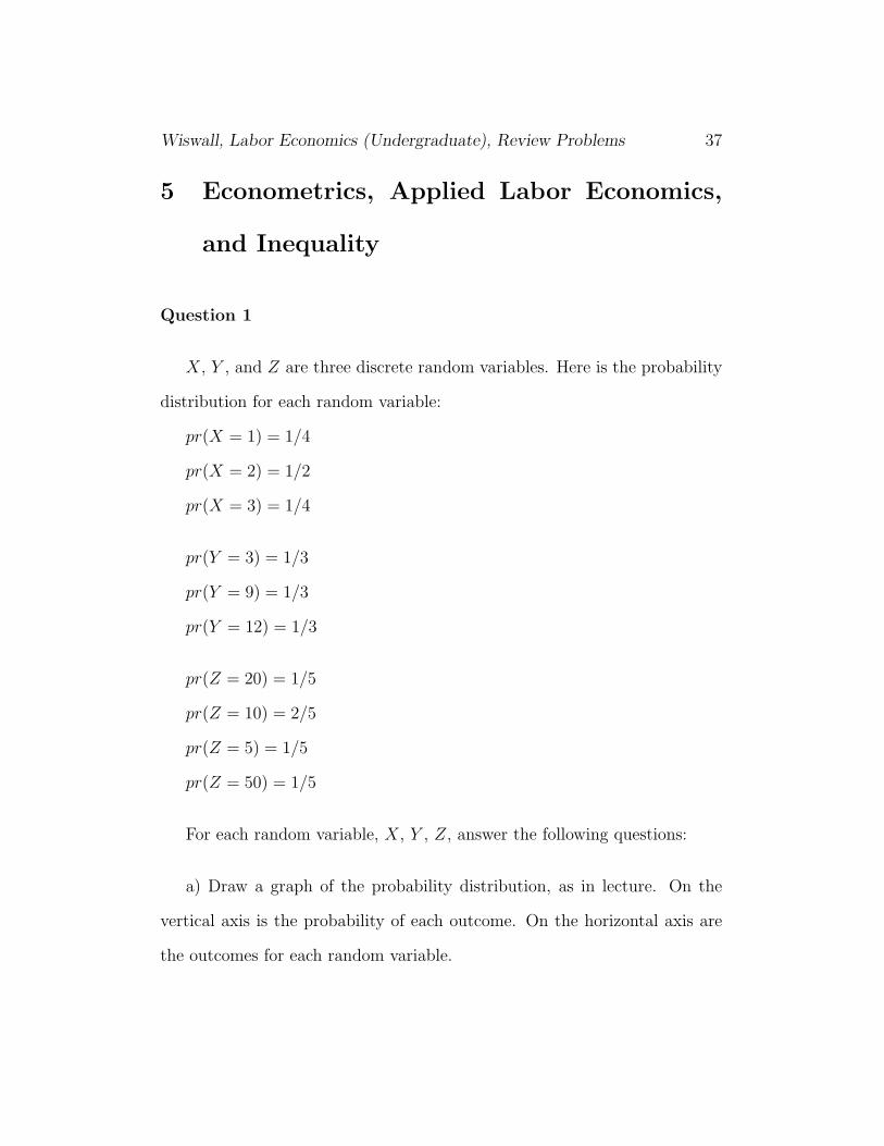
Question 1

X, Y , and Z are three discrete random variables. Here is the probability

distribution for each random variable:

pr(X = 1) = 1/4

pr(X = 2) = 1/2

pr(X = 3) = 1/4

pr(Y = 3) = 1/3

pr(Y = 9) = 1/3

pr(Y = 12) = 1/3

pr(Z = 20) = 1/5

pr(Z = 10) = 2/5

pr(Z = 5) = 1/5

pr(Z = 50) = 1/5

For each random variable, X, Y , Z, answer the following questions:

a) Draw a graph of the probability distribution, as in lecture. On the

vertical axis is the probability of each outcome. On the horizontal axis are

the outcomes for each random variable.


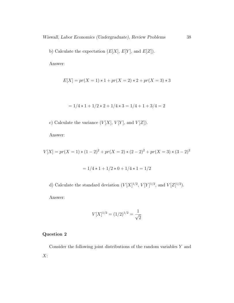
b) Calculate the expectation (E[X], E[Y ], and E[Z]).

Answer:

E[X] = pr(X = 1) ∗ 1 + pr(X = 2) ∗ 2 + pr(X = 3) ∗ 3

= 1/4 ∗ 1 + 1/2 ∗ 2 + 1/4 ∗ 3 = 1/4 + 1 + 3/4 = 2

c) Calculate the variance (V [X], V [Y ], and V [Z]).

Answer:

V [X] = pr(X = 1) ∗ (1 − 2)2 + pr(X = 2) ∗ (2 − 2)2 + pr(X = 3) ∗ (3 − 2)2

= 1/4 ∗ 1 + 1/2 ∗ 0 + 1/4 ∗ 1 = 1/2

d) Calculate the standard deviation (V [X]1/2, V [Y ]1/2, and V [Z]1/2).

Answer:

V [X]1/2 = (1/2)1/2 =1√2

Question 2

Consider the following joint distributions of the random variables Y and

X:


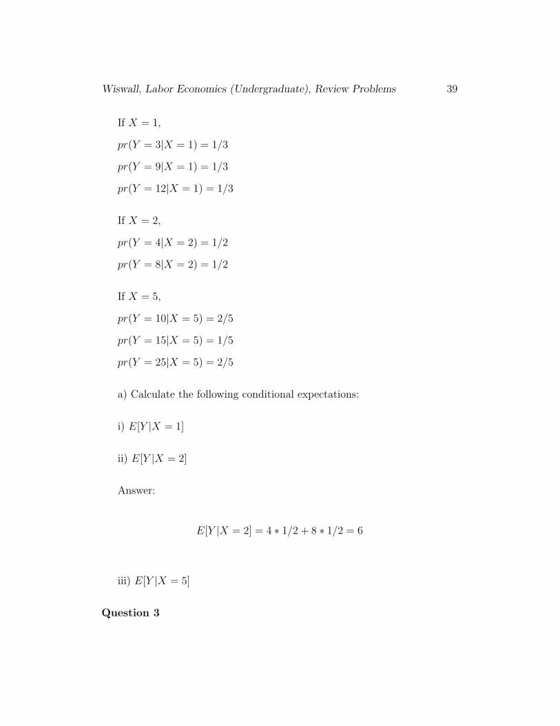
If X = 1,

pr(Y = 3|X = 1) = 1/3

pr(Y = 9|X = 1) = 1/3

pr(Y = 12|X = 1) = 1/3

If X = 2,

pr(Y = 4|X = 2) = 1/2

pr(Y = 8|X = 2) = 1/2

If X = 5,

pr(Y = 10|X = 5) = 2/5

pr(Y = 15|X = 5) = 1/5

pr(Y = 25|X = 5) = 2/5

a) Calculate the following conditional expectations:

i) E[Y |X = 1]

ii) E[Y |X = 2]

Answer:

E[Y |X = 2] = 4 ∗ 1/2 + 8 ∗ 1/2 = 6

iii) E[Y |X = 5]

Question 3


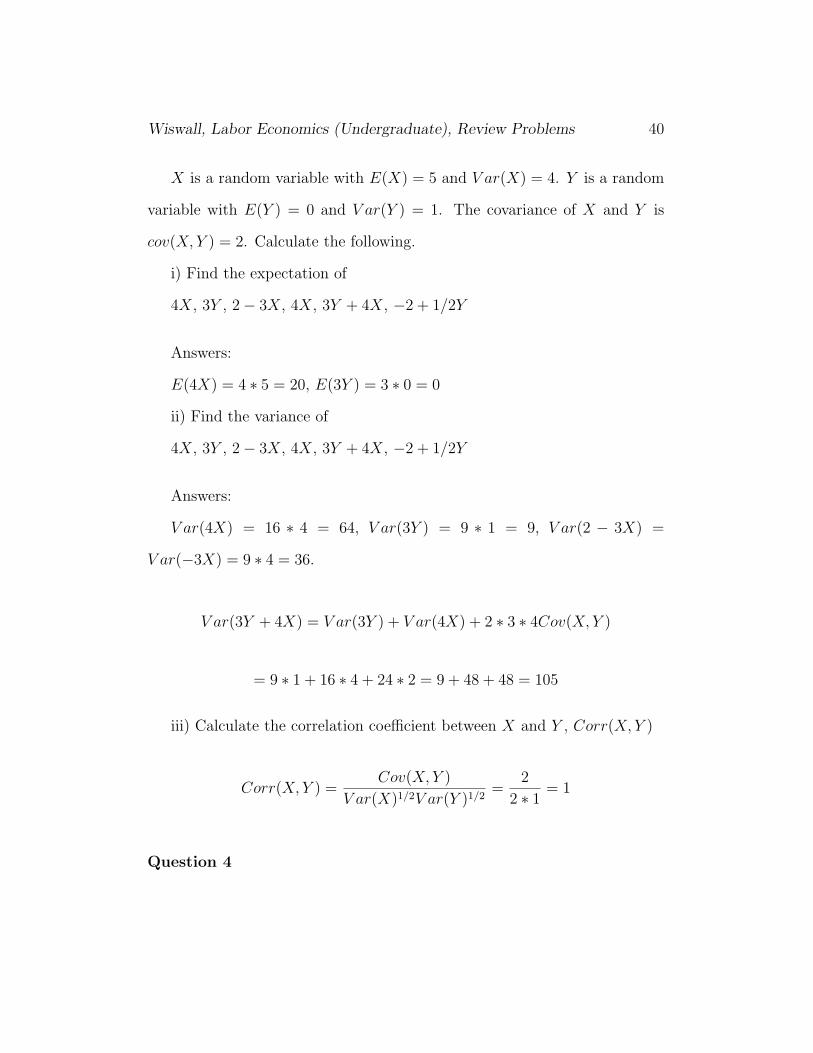
X is a random variable with E(X) = 5 and V ar(X) = 4. Y is a random

variable with E(Y ) = 0 and V ar(Y ) = 1. The covariance of X and Y is

cov(X, Y ) = 2. Calculate the following.

i) Find the expectation of

4X, 3Y , 2 − 3X, 4X, 3Y + 4X, −2 + 1/2Y

Answers:

E(4X) = 4 ∗ 5 = 20, E(3Y ) = 3 ∗ 0 = 0

ii) Find the variance of

4X, 3Y , 2 − 3X, 4X, 3Y + 4X, −2 + 1/2Y

Answers:

V ar(4X) = 16 ∗ 4 = 64, V ar(3Y ) = 9 ∗ 1 = 9, V ar(2 − 3X) =

V ar(−3X) = 9 ∗ 4 = 36.

V ar(3Y + 4X) = V ar(3Y ) + V ar(4X) + 2 ∗ 3 ∗ 4Cov(X, Y )

= 9 ∗ 1 + 16 ∗ 4 + 24 ∗ 2 = 9 + 48 + 48 = 105

iii) Calculate the correlation coefficient between X and Y , Corr(X, Y )

Corr(X, Y ) =Cov(X, Y )

V ar(X)1/2V ar(Y )1/2=

2

2 ∗ 1= 1

Question 4


A survey collected information from 10 respondents. Each respondent

was asked their hourly wage rate (w), their gender (M = 1 if male, G = 0

if female), whether they have a college degree (D = 1 if they have a college

degree, D = 0 if they do not), and their hours of work (h).

Here is the data: (w,M,D, h)

Person 1: (12, 1, 0, 20), Person 2: (8, 1, 0, 40), Person 3: (10, 1, 0, 35),

Person 4: (25, 1, 1, 38), Person 5: (60, 1, 1, 45),

Person 6: (8, 0, 0, 30), Person 7: (14, 0, 0, 15), Person 8: (7, 0, 0, 40),

Person 9: (48, 0, 1, 50), Person 10: (8, 0, 1, 20).

Calculate the following sample descriptive statistics. You may want to

use a spreadsheet program (e.g. Excel).

i)

Mean wage for all respondents

Answer:

w = 1/10 ∗ (12 + 8 + 10 + 25 + 60 + 8 + 14 + 7 + 48 + 8) = 20

Mean wage for males

Mean wage for females

Mean wage for college graduates

Mean wage for non-college graduates

Mean wage for male college graduates


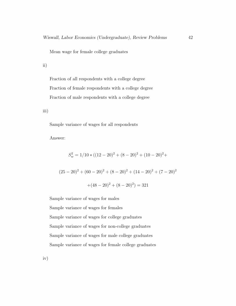
Mean wage for female college graduates

ii)

Fraction of all respondents with a college degree

Fraction of female respondents with a college degree

Fraction of male respondents with a college degree

iii)

Sample variance of wages for all respondents

Answer:

S2w = 1/10 ∗ ((12 − 20)2 + (8 − 20)2 + (10 − 20)2+

(25 − 20)2 + (60 − 20)2 + (8 − 20)2 + (14 − 20)2 + (7 − 20)2

+(48 − 20)2 + (8 − 20)2) = 321

Sample variance of wages for males

Sample variance of wages for females

Sample variance of wages for college graduates

Sample variance of wages for non-college graduates

Sample variance of wages for male college graduates

Sample variance of wages for female college graduates

iv)


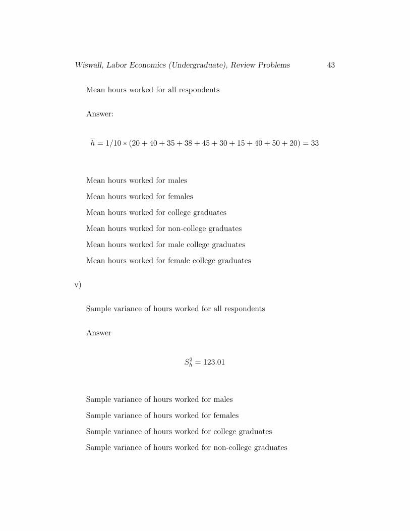
Mean hours worked for all respondents

Answer:

h = 1/10 ∗ (20 + 40 + 35 + 38 + 45 + 30 + 15 + 40 + 50 + 20) = 33

Mean hours worked for males

Mean hours worked for females

Mean hours worked for college graduates

Mean hours worked for non-college graduates

Mean hours worked for male college graduates

Mean hours worked for female college graduates

v)

Sample variance of hours worked for all respondents

Answer

S2h = 123.01

Sample variance of hours worked for males

Sample variance of hours worked for females

Sample variance of hours worked for college graduates

Sample variance of hours worked for non-college graduates


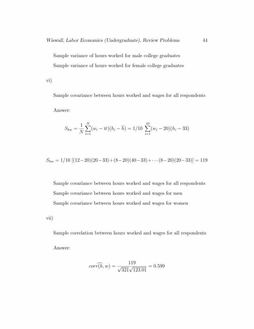
Sample variance of hours worked for male college graduates

Sample variance of hours worked for female college graduates

vi)

Sample covariance between hours worked and wages for all respondents

Answer:

Shw =1

N

N∑i=1

(wi − w)(hi − h) = 1/1010∑i=1

(wi − 20)(hi − 33)

Shw = 1/10 [(12−20)(20−33)+(8−20)(40−33)+· · · (8−20)(20−33)] = 119

Sample covariance between hours worked and wages for all respondents

Sample covariance between hours worked and wages for men

Sample covariance between hours worked and wages for women

vii)

Sample correlation between hours worked and wages for all respondents

Answer:

corr(h,w) =119√

321√

123.01= 0.599


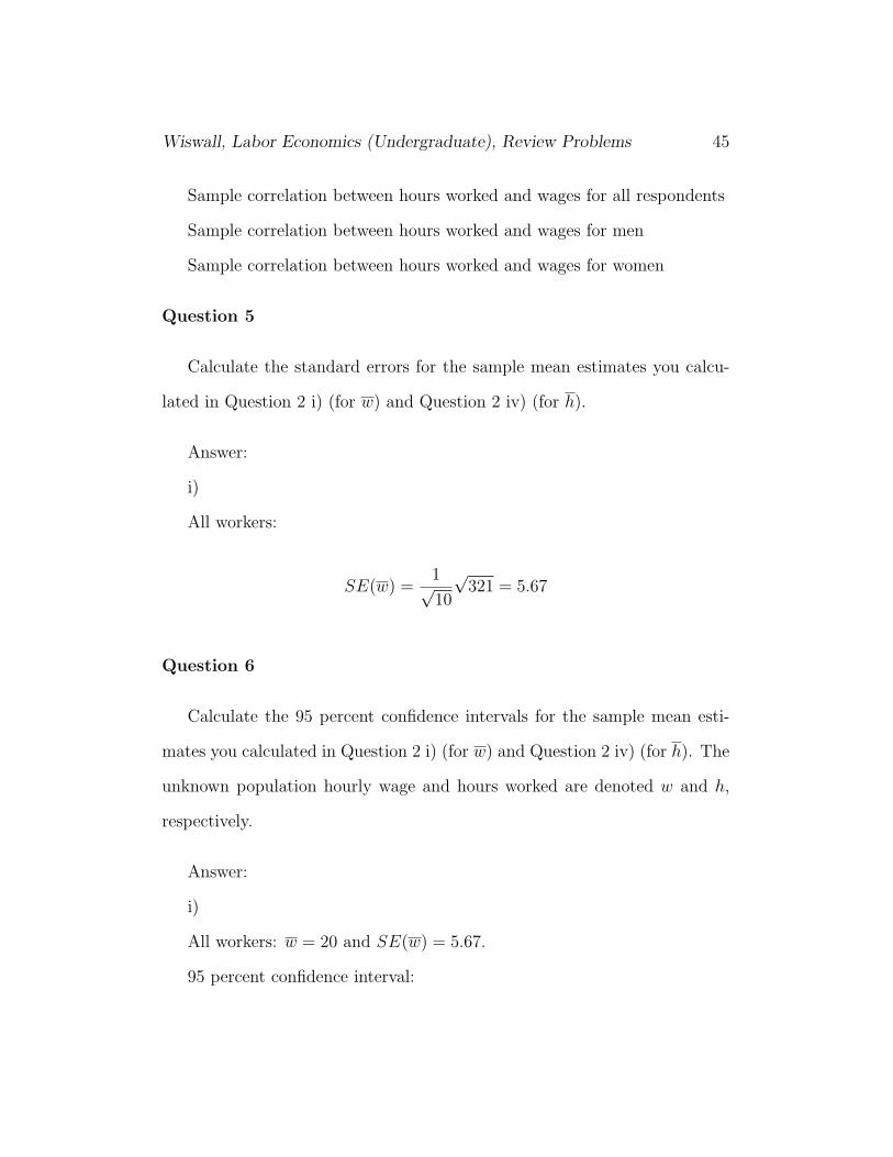
Sample correlation between hours worked and wages for all respondents

Sample correlation between hours worked and wages for men

Sample correlation between hours worked and wages for women

Question 5

Calculate the standard errors for the sample mean estimates you calcu-

lated in Question 2 i) (for w) and Question 2 iv) (for h).

Answer:

i)

All workers:

SE(w) =1√10

√321 = 5.67

Question 6

Calculate the 95 percent confidence intervals for the sample mean esti-

mates you calculated in Question 2 i) (for w) and Question 2 iv) (for h). The

unknown population hourly wage and hours worked are denoted w and h,

respectively.

Answer:

i)

All workers: w = 20 and SE(w) = 5.67.

95 percent confidence interval:


20 − 5.67 ∗ 2 ≤ w ≤ 20 + 5.67 ∗ 2

8.66 ≤ w ≤ 31.34

Question 7

Using the 95 percent confidence intervals you calculated in Question 4,

test the hypothesis (for w and h) that the population value is 0.

Answer:

All workers:

0 is outside the 95 percent confidence interval. We reject the hypothesis

that w is 0 at the 95 percent confidence level.

Question 8

Our regression model is

Y = β0 + β1X1 + β2X2 + εi

Assume the assumptions of the neo-classical regression model hold.

a) Using the regression model, calculate the following conditional expec-

tations:


i)

E[Y |X1 = 2, X2 = 3]

Answer:

E[Y |X1 = 2, X2 = 3] = β0 + β12 + β23 + E[ε|X1 = 2, X2 = 3]

Under the assumptions of the neo-classical regression model, X1 and X2

are independent of ε. Hence,

E[ε|X1 = 2, X2 = 3] = 0

Therefore, we can write

E[Y |X1 = 2, X2 = 3] = β0 + β12 + β23

ii)

E[Y |X1 = 0, X2 = 3]

iii)

E[Y |X1 = 2, X2 = 0]

iv)

E[Y |X1 = 1, X2 = 1]


v)

E[Y |X1 = 0, X2 = 0]

vi)

E[Y |X1 = −1, X2 = −3]

b) Now assume that X1 and X2 are not independent of ε. Re-calculate

the conditional expectations in part a).

Answer:

For i)

Since ε is not independent of X1 or X2, we can only write

E[Y |X1 = 2, X2 = 3] = β0 + β12 + β23 + E[ε|X1 = 2, X2 = 3]

c) Now assume we know the population parameters. β0 = 1/2, β1 = 2,

and β2 = −1. Assume X is independent of ε. Re-calculate the conditional

expectations in part a).

Answer:

For i)

E[Y |X1 = 2, X2 = 3] = 1/2 + 2 ∗ 2 + (−1) ∗ 3 = 9/2 − 6/2 = 3/2


Question 9

Assume the same regression model as in Question 1.

For three different samples, we calculate estimates of the regression model

parameters using OLS (standard errors are in parentheses):

Estimate Set A: β0 = 1 (0.5), β1 = 3 (1.5), β2 = −2 (1.5).

Estimate Set B: β0 = 2 (0.5), β1 = 0 (2), β2 = 3 (2).

Estimate Set C: β0 = 0.5 (1), β1 = 0.5 (0.1), β2 = 1 (0.5).

a) For each of the three sets estimates, predict the level of Y given the

following four sets of values for X1 and X2.

i) X1 = 1, X2 = 1.

Answer:

Prediction of Y using Estimate A is

Y = β0 + β1X1 + β2X2 = 1 + 3 ∗ 1 + (−2) ∗ 1 = 4 − 2 = 2

ii) X1 = 0, X2 = 0.

iii) X1 = 0, X2 = 1.

iv) X1 = 4, X2 = 5.


b) For each set of parameter estimates, describe what the estimated re-

lationship is between the X1 and X2 variables and the Y .

For Estimate A, β1 = 3 indicates that higher levels of X1 increase Y

(positive correlation). β2 = −2 indicates that higher levels of X2 decrease Y

(negative correlation).

c) For each parameter estimate and for each set of estimates, calculate the

95 percent confidence interval (3 x 3 = 9 total confidence intervals). Assume

the critical value is 2.

Answer:

95 percent confidence interval for β0 using Estimate A:

1 − 0.5 ∗ 2 ≤ β0 ≤ 1 + 0.5 ∗ 2

0 ≤ β0 ≤ 2

d) For each parameter estimate and for each set of estimates, test the

hypothesis at the 95 percent confidence level that each parameter is zero (3

x 3 = 9 total hypothesis tests).

For β0 using the estimate from Estimate A, we cannot reject the hy-

pothesis that β0 = 0. 0 is within the the 95 percent confidence interval we

calculated in part b).


e) For each parameter estimate and for each set of estimates, test the

hypothesis at the 95 percent confidence level that each parameter is 3 (3 x 3

= 9 total hypothesis tests).

For β0 using the estimate from Estimate A, we can reject the hypothesis

that β0 = 3. 3 is not within the the 95 percent confidence interval we

calculated in part b).

Question 10

Consider the following research questions and accompanying regression

models.

Research Design A: What is the effect of the size of the police force on

crime rates?

crimei = β0 + β1policei + εi,

where crimei is the crime rate for city i and policei is the size of the police

force for city i.

Research Design B: What is the effect of the number of immigrants in an

individual’s city on that person’s wages?

wi = β0 + β1immigri + εi,


where wi is individual i’s wage and immigri is the number of immigrants

in individual i’s city.

Research Design C: What is the effect of business failures on unemploy-

ment?

faili = β0 + β1unempli + εi,

where faili is the number of firms that went out of business in city i and

unempli is the unemployment rate in city i.

a) For each of the research designs, write down the specific equations for

the OLS estimator.

Answer:

For Research Design B:

β1 =1N

∑Ni=1(wi − w)(immigri − immigr)1N

∑Ni=1(immigri − immigr)2

β0 = w − β1immigr,

where immigr and w are the respective sample means of these two vari-

ables.


b) Write the specific assumption which are required for the OLS estimator

to be unbiased.

Answer:

For Research Design B:

The important assumption is that the X variable is independent of ε. In

this case, the number of immigrants in a city must be independent of all of

the other factors which affect an individual’s wage (represented by εi).

c) For each of the research designs, describe the potential self-selection

bias if we use OLS to estimate these regression models.

d) For each of the research designs, suggest at least 2 different ways to

solve the self-selection bias.

Question 11

Consider two different economies. For each economy, we have a random

sample of 13 hourly wage observations:

Economy A: 10, 10, 10, 15, 12, 20, 24, 25, 30, 40, 40, 40, 40

Economy B: 8, 8, 8, 15, 25, 30, 40, 70, 80, 90, 90, 90, 90

a) For each economy, calculate the following measures of inequality:

i) 90-10 differential

Answer:


Because of the few number of wage observations (N = 10), it’s difficult

to find the exact 90th and 10th percentiles of earnings.

For Economy A:

The 90th percentile is about W90 = 40

The 10th percentile is about W10 = 10

D90−10 =40

10= 4,

ii) 50-10 differential

iii) 70-30 differential

iv) standard deviation

b) Which economy has the higher level of inequality?

Question 12

Assume there are two groups of people: group A and group B. There

are two education levels: col (college degree) and high (no college degree).

We collect two random samples of 10 people for each group. Each data

observation consists of an education level and an hourly wage. Here is our

data:

Group A: (col, 30), (col, 50), (col, 35), (high, 10), (high, 20), (high, 8),

(high, 25), (high, 15), (high, 20), (high, 10)


Group B: (col, 15), (col, 60), (col, 40), (col, 35), (col, 50) (high, 12),

(high, 20), (high, 30), (high, 25), (high, 20)

a) For each group, calculate the average wage.

b) Calculate the fraction of each group with a college degree.

c) Calculate the average wage for each group by schooling level.

d) Calculate the 90-10 and 50-10 differential for the whole population

(both groups).

e) Calculate the 90-10 and 50-10 differential for each group separately.

f) Calculate a decomposition of the difference in wages between the groups

as in the lecture notes.

Documents

1 Overview of Labor Markets and Labor De- mand Labor Economics (Undergraduate), Review Problems 1 1 Overview of Labor Markets and Labor De-mand Question 1: Show in a labor supply and