Embed Size (px)
Citation preview

1
Optimization of Amplify-and-Forward
Multicarrier Two-Hop Transmission
Wenyi Zhang, Member, IEEE, Urbashi Mitra, Fellow, IEEE, and Mung Chiang,
Member, IEEE
Abstract
In this paper, frequency-domain relay processing in a two-hop transmission system is investigated.
The relay is constrained to be “non-regenerative”; that is, the relay is only allowed to perform symbol-
by-symbol memoryless transformation of its received signals. Multicarrier modulation, e.g., orthogonal
frequency division multiplexing (OFDM), is utilized to convert each hop link into a collection of non-
interfering parallel subcarriers. In contrast to conventional scalar amplify-and-forward (AF) relays that
scale all the subcarriers uniformly, it is possible to suppress relay noise and to exploit frequency-domain
diversity by optimizing the relay scaling coefficients of different subcarriers jointly with subcarrier
power allocation at the source transmitter. Although the end-to-end achievable rate is a non-concave
function of the power allocation vectors, its optimization is accomplished with an algorithm whose
computational complexity grows linearly with the number of subcarriers, by utilizing a structural property
of the problem. Further motivated by the problem structure, a suboptimal algorithm with even lower
complexity is also proposed, in which each hop link performs waterfilling separately over a selected
subset of subcarriers. For hop links with a frequency-flat channel profile, the maximum achievable rate
is explicitly derived as is the associated optimization. For hop links with Rayleigh fading frequency-
domain channel profiles, numerical simulation results are presented, and it is illustrated that the proposed
low-complexity suboptimal algorithm usually achieves near-optimal performance.
The work of W. Zhang and U. Mitra was supported in part by NSF OCE-0520324. Preliminary results in this paper have
appeared in part in [1].
W. Zhang was with the Ming Hsieh Department of Electrical Engineering, University of Southern California, Los Angeles,
CA, and he is now with Qualcomm Research Center, San Diego, CA. (Email: [email protected]).
U. Mitra is with the Ming Hsieh Department of Electrical Engineering, University of Southern California, Los Angeles, CA.
(Email: [email protected]).
M. Chiang is with Department of Electrical Engineering, Princeton University, Princeton, NJ. (Email:
August 11, 2008 DRAFT

2
Index Terms
amplify-and-forward, multicarrier, multihop network, non-convex optimization, relay network, OFDM,
rate optimization
I. INTRODUCTION
In a multihop transmission system, information flows through hop links connected by re-
lays (repeaters) from a source to a destination. Such systems have been persistently studied
since the early days of communication engineering; see, e.g., [2]-[6] and references therein for
an incomplete list covering various aspects of multihop transmission.1 Multihop transmission
dramatically benefits the per-hop signal-to-noise ratio (SNR) by splitting a long transmission
range into multiple shorter hops, and thus is an indispensable solution in various systems like
digital subscriber lines (DSL), wireless mesh networks, satellite networks, underwater acoustic
networks, low-power sensor networks, and optical networks.
Among different processing techniques at relay nodes, the decode-and-forward (DF) scheme
achieves the capacity of a multihop transmission system, as can be readily argued by a cut-
set bounding technique [8]. In certain practical systems, however, due to other considerations
like complexity (e.g., [7]) or latency (e.g., [6]), nodes may adopt simpler signal processing
techniques, in particular, the so-called non-regenerative relaying in which only symbol-by-symbol
memoryless transformation is allowed. In single-carrier modulation, the non-regenerative relay
processing is conventionally implemented by an amplify-and-forward (AF) scheme, in which
the received signal is linearly scaled by a scaling coefficient and then transmitted toward the
destination.
The scalar AF scheme fails to suppress the relay noise, and fails to exploit potential frequency
diversity exhibited by the hop links, especially in multicarrier modulation like orthogonal fre-
quency division multiplexing (OFDM) which decomposes each hop link into a collection of non-
interfering parallel subcarriers. In this paper, we investigate the problem of jointly optimizing
the relay AF scaling coefficient for each subcarrier in addition to the subcarrier power allocation
at the source transmitter. For tractability and simplicity, we focus on a two-hop system with
1Our multihop model only considers transmission between adjacent nodes, in contrast to the classical relay channel model
where the source and the destination are directly connected [8]. Such a hop-by-hop transmission is a consequence either of
physical constraints (e.g., wireline), or of practical design (e.g., treating signals from remote nodes as interference).
August 11, 2008 DRAFT

3
a single relay node. The objective of the optimization is to maximize the end-to-end achiev-
able information rate, expressed as the mutual information between the source inputs and the
destination outputs, subject to source power allocation and relay processing constraints.
Interestingly, exactly the same rate-maximization problem has been formulated in [11], stem-
ming from the general problem of designing optimal linear source precoder and linear relay
transformers for a two-hop system equipped with multiple antennas. Note that through singular-
value decomposition (SVD), multiple-port channel matrices can be decoupled into multicarrier
parallel channels. The end-to-end achievable rate, unfortunately, is a non-concave function with
power allocation vectors, and thus cannot be readily maximized utilizing techniques like the
interior point method or other methods relying on the sufficiency of the Karush-Kuhn-Tucker
(KKT) conditions (see, e.g., [9]) in characterizing optimal solutions. Due to this difficulty, no
optimal solution was provided in [11]. On the other hand, by extending the proof techniques
in an earlier work [10], the authors of [11] established an important structural property of the
optimal solution. For the multicarrier system considered here, the structural property implies
that the optimal linear relay processing consists of two stages. In the first stage, the incoming
subcarriers from the source-relay link should be permuted, such that their rankings with respect
to their channel gain magnitudes are matched to the outgoing subcarriers of the relay-destination
link. In this way, strong subcarriers are further strengthened, and weak subcarriers are further
weakened. This is somewhat analogous to maximal-ratio combining in diversity reception [12].
Subsequently, the second stage corresponds to a collection of per-subcarrier linear AF, and is
subject to optimization.
In this paper, we successfully accomplish the optimization of the end-to-end achievable rate,
and the corresponding algorithm is a linear search procedure with computational complexity
that is linear with the number of subcarriers. Although the optimization problem lacks the
desired convexity properties, it is still possible to obtain its solution through an exhaustive
enumeration of all of its stationary and boundary points. Generally speaking, the number of
those candidate points grows exponentially with the size of the problem (characterized by the
number of subcarriers) so that an exhaustive enumeration is practically infeasible. Fortunately,
by utilizing the aforementioned structural property regarding optimal permutation as established
in [10] and [11], we find that the exhaustive enumeration can be reduced to a linear search, in
which, at each step, we compute the maximum rate under the constraint that a certain number
of weak subcarriers are not allocated any power.
August 11, 2008 DRAFT

4
The optimal algorithm involves solving a series of cubic equations, which still may not be
pragmatic. Further motivated by the structural property and by a simple heuristic, we propose
a suboptimal algorithm, in which each hop link simply performs waterfilling separately over a
linearly searched subset of strong subcarriers, thus avoiding the occurrence of cubic equations. A
surprising observation made empirically via simulations is that the low-complexity, suboptimal
algorithm usually achieves near-optimal performance, with negligible rate loss. We note that all
the developments in the paper can readily be applicable to a system whose transceivers have
multiple input/output ports, as in [10] and [11].
We further present analytical results in the special case of frequency-flat channel profile, i.e.,
with common channel gain for each subcarrier in a link. For this case, the optimal algorithm and
the low-comlexity suboptimal algorithm coincide and the maximum rate is achieved by an on-off
power allocation scheme over the subcarriers. This phenomenon precisely reflects the impact of
the lack of convexity in the problem. Consequently, even if each hop link is wideband with
sufficiently many subcarriers available, it is often optimal not to use all of these subcarriers. In
contrast, for single-hop transmission, it is always optimal to uniformly allocate power among
all subcarriers in the wideband regime.
The remainder of this paper is organized as follows. Section II introduces the two-hop system
model and formulates the rate maximization problem. Section III establishes the linear search
algorithm that yields the optimal solution to the rate maximization problem. Section IV motivates
and describes the low-complexity suboptimal algorithm. Section V presents results and discussion
on the case where the hop links exhibit frequency-flat channel profile. Section VI generalizes
the problem to the limit of continuous frequency-domain response. Section VII presents results
and discussion from numerical simulation, for subcarriers whose channel coefficients resemble
Gaussian random variables. Finally Section VIII concludes the paper. As a convention, all
logarithms are to base e, and all rates are measured by nats.
II. SYSTEM MODEL AND PROBLEM FORMULATION
In this paper, we consider a two-hop system, with each hop link being a multicarrier modulated
channel consisting of N subcarriers. For simplicity, we assume that the channel responses
remain static throughout transmission, and that the inter-carrier interference between subcarriers
is negligible. With the time index suppressed, the channel equation for subcarrier n is written
August 11, 2008 DRAFT

5
in discrete-time baseband form as
Ym[n] = hm[n]Xm[n] + Zm[n], n = 1, . . . , N, (1)
with m = 1 denoting the source-relay link and m = 2 denoting the relay-destination link. For
each hop link, the complex-valued inputs Xm[·] have an average power constraint across the N
subcarriers,
E
[N∑
n=1
|Xm[n]|2]
= Pm, m = 1, 2. (2)
The additive noise random variables Zm[·] are modeled as circularly symmetric complex Gaus-
sian, with zero mean and variance σ2m for m = 1, 2. We further assume that Zm[·] are mutually
independent across time and across subcarriers (i.e., “white” in both time and frequency). The
complex-valued channel profile coefficients, hm[·], are modeled as deterministic and known
throughout transmission, in light of the static channel assumption.
The relay node that joins the two hop links is the cascade of a permutation stage and an
amplification stage, as illustrated in Figure 1. In its operation, the relay first demodulates the
time-domain received signal and obtains the signals over the N subcarriers from the source-
relay link, Y1 =(Y1[1], . . . ,Y1[N ]
)T, accomplished by standard OFDM demodulation, including
removing the cyclic prefix, serial-parallel conversion, and discrete Fourier transform (DFT). In
the subsequent permutation stage, the relay permutes the elements of the Y1 vector according to
a deterministic permutation function π(·), thus obtaining
Y(π)1 =
(Y1[π(1)], . . . ,Y1[π(N)]
)T. (3)
Taking Y(π)1 as its input vector, the amplification stage consists of N linear amplifiers each
corresponding to one element in Y(π)1 . The output stage vector is thus
X2 =(c[1]Y1[π(1)], . . . , c[N ]Y1[π(N)]
)T. (4)
Note that the amplification coefficients c[·] can be different. The optimal and suboptimal se-
lections of these coefficients will be one of the major contributions of this work. Finally, the
relay forms its time-domain transmitted signal for transmission over the relay-destination link,
by performing standard OFDM modulation (inverse DFT, adding the cyclic prefix, and parallel-
to-serial conversion) on X2.
August 11, 2008 DRAFT

6
The received signal at the destination for subcarrier n is denoted Y2[n]; the end-to-end channel
equation for Y2[n] is given by,
Y2[n] = h2[n]X2[n] + Z2[n]
= h2[n]c[n]Y1[π−1(n)] + Z2[n]
= h2[n]c[n](h1[π
−1(n)]X1[π−1(n)] + Z1[π
−1(n)])
+ Z2[n]
= h1[π−1(n)]h2[n]c[n]X1[π
−1(n)] +(h2[n]c[n]Z1[π
−1(n)] + Z2[n]). (5)
To proceed, it is more convenient to rewrite Xm[n] =√
γm[n]Xm[n], such that each Xm[n]
has zero mean and unit variance, and such that the nonnegative power allocation vector γm
=(γm[1], . . . , γm[N ]
)T satisfies the average power constraint∑N
n=1 γm[n] = Pm, for m = 1, 2.
With this notation, the amplification coefficients at the relay satisfy
|c[n]|2 =γ2[n]
|h1[π−1(n)]|2γ1[π−1(n)] + σ21
, n = 1, . . . , N. (6)
Consequently, the end-to-end channel equation (5) can be normalized and reduced to
Y2[n] =√
ρ[n]X1[π−1(n)] + Z[n], n = 1, . . . , N, (7)
where Z[n] is a circularly symmetric complex Gaussian random variable with zero mean and
unit variance, and
ρ[n] =|h1[π
−1(n)]|2|h2[n]|2γ1[π−1(n)]γ2[n]
|h1[π−1(n)]|2γ1[π−1(n)]σ22 + |h2[n]|2γ2[n]σ2
1 + σ21σ
22
(8)
characterizes the end-to-end SNR for Y2[n].
To simplify notation, in the remainder of this paper, we introduce
am[n] =|hm[n]|2
σ2m
, for m = 1, 2 (9)
as the normalized channel gains, and rewrite the per-subcarrier SNR ρ[n] as
ρ[n] =a1[π
−1(n)]a2[n]γ1[π−1(n)]γ2[n]
a1[π−1(n)]γ1[π−1(n)] + a2[n]γ2[n] + 1. (10)
For a specified permutation function π(·) and power allocation vectors γm
, m = 1, 2, the the-
oretically maximum information rate that is achievable over the end-to-end two-hop multicarrier
system is
R(π(·), γ
)=
N∑n=1
log (1 + ρ[n]) . (11)
August 11, 2008 DRAFT

7
To achieve the rate R(π(·), γ
), we assume that all the inputs over the N subcarriers resemble
mutually independent and circularly symmetric complex Gaussian random variables, and that
optimum encoding/decoding procedures are utilized. Consequently, the problem that we seek to
solve in this paper is to maximize the rate, as follows,
max R(π(·), γ
)=
N∑n=1
log (1 + ρ[n]) , (12)
s.t.N∑
n=1
γm[n] = Pm, m = 1, 2, (13)
variables: π(·), γ, (14)
where ρ[n] is given by Equation (10).
Remark 1: In the rate function in Equation (12), we implicitly ignore the rate loss due to
the cyclic prefix if the multicarrier modulation is implemented by OFDM. Such a loss becomes
negligible as we increase the number of subcarriers such that N is much larger than the channel
delay spread.
Remark 2: The preceding description of the channel model accommodates both full-duplex
and half-duplex relay transceivers. For the half-duplex case, we only need to properly scale the
model, namely, double the average power constraint (Pm, m = 1, 2) and halve the resulting
information rate R(π(·), γ
).
III. STRUCTURE AND ALGORITHM FOR OPTIMAL SOLUTION
The optimization problem (12) can be decoupled into two separate subproblems: a discrete
optimization that yields the optimum permutation function π∗(·), and a continuous optimization
that yields the optimum power allocation vectors γ∗m
, m = 1, 2. At first glance, optimizing
π(·) requires an exhaustive search over all possible permutations of {1, . . . , N}, whose com-
plexity grows exponentially with N because the total number of possible permutations is N !.
Fortunately, by exploiting matrix theory, the authors of [10], [11] were able to circumvent the
exhaustive enumeration and prove that the optimal permutation function yields a rather simple
form. Furthermore, in this paper, we depart from characterization of optimal solution structures
to practical algorithm implementations.
To rephrase the result for our problem in this paper, it is convenient to introduce a ranking
operator instead of the permutation function. For a vector, the ranking operator is defined as
follows.
August 11, 2008 DRAFT

8
Definition 1: For a length-N vector s = {s[n]}Nn=1 whose elements are all nonnegative, the
ranking operator R is defined such that R(s) = {sR[n]}Nn=1 is another length-N vector, whose
elements are obtained by permuting the elements of s, with sR[n1] ≥ sR[n2] for arbitrary n1 < n2.
Having defined the ranking operator, we state the optimal permutation function in the following
lemma.
Lemma 2: (see [10, Sec. III] and [11, Thm. 1])
For the two-hop transmission system model in Section II, the permutation function π∗(·) that
solves problem (12) is an identity function π(n) = n if we apply the ranking operator R to
{a1[n]}Nn=1 and {a2[n]}N
n=1 simultaneously.
In words, Lemma 2 states that if we rank and re-index the subcarriers of each hop link
according to the rankings of subcarriers’ channel gain magnitudes, in a descending order, then
no further permutation is needed for achieving the maximum transmission rate. Throughout the
remainder of this paper, we shall adhere to this ranking (therefore suppressing the superscript
·R in {aRm[n]}N
n=1), m = 1, 2, thus reducing the problem to one of power allocation only. Now
it is convenient to rewrite the achievable rate in Equation (12), utilizing Equation (10), as
R(γ)
=N∑
n=1
log (1 + a1[n]γ1[n]) +N∑
n=1
log (1 + a2[n]γ2[n])
−N∑
n=1
log (1 + a1[n]γ1[n] + a2[n]γ2[n]) , (15)
where we once again emphasize that the channel profile coefficients have been ranked and re-
indexed such that a1[1] ≥ a1[2] ≥ . . . ≥ a1[N ] and a2[1] ≥ a2[2] ≥ . . . ≥ a2[N ].
It is easy to verify that R(γ)
is not a concave function, and thus its maximization cannot be
solved by techniques like the interior point method or other methods relying on the sufficiency
of the Karush-Kuhn-Tucker (KKT) conditions in characterizing optimal solutions. Actually,
the KKT conditions can only yield all possible candidates of the optimal solution, whereas
enumerating all those candidate solutions is still overwhelming in complexity. What can be said
is that, in the optimal solution, for each subcarrier index n ∈ {1, . . . , N}, we have either
∂J(γ)
∂γ1[n]=
∂J(γ)
∂γ2[n]= 0; (16)
or, γ1[n] = γ2[n] = 0, (17)
August 11, 2008 DRAFT

9
where the Lagrangian J(γ)
is
J(γ)
= R(γ)− λ1
(N∑
n=1
γ1[n]− P1
)− λ2
(N∑
n=1
γ2[n]− P2
), (18)
for arbitrary λm ∈ R, m = 1, 2. The vanishing partial derivatives in Equation (16), are from the
first-order optimality test. In Equation (17), the variables are on the boundary of the feasible
set, and we note that if either of γm[n], m = 1, 2, vanishes, the other also has to be so in the
optimal solution.
Applying Lemma 2, we obtain that the optimal power allocation solution exhibits the following
truncated structure.
Lemma 3: For the optimal power allocation vectors γ∗m
, m = 1, 2, there exists an integer
K ∈ {1, . . . , N}, such that
γ∗m[n] > 0, ∀n ≤ K (19)
and γ∗m[n] = 0, otherwise, (20)
for m = 1, 2.
Proof: This is a direct consequence of the ranking with a1[1] ≥ a1[2] ≥ . . . ≥ a1[N ] and
a2[1] ≥ a2[2] ≥ . . . ≥ a2[N ]. Actually, assume that there exist n1 and n2, n1 < n2, with at
least one of the inequalities am[n1] ≥ am[n2], m = 1, 2, being strict, and with γ∗m[n1] = 0 and
γ∗m[n2] > 0, m = 1, 2, in the optimal solution. Then if we exchange the values of γ∗m[n1] and
γ∗m[n2], the resulting achievable rate will always be increased because we have am[n1] ≥ am[n2],
m = 1, 2, with at least one of them being strict, and because R(γ)
is a monotonically increasing
function with each γm[·] ≥ 0, m = 1, 2.�
The implication of Lemma 3 is that we can adopt a linear search procedure to seek the optimal
power allocation vectors and the maximum achievable rate. Due to the truncated structure of the
optimal solution, all the power allocation variables satisfying the boundary condition (17) are
grouped together around the weak subcarriers, and all the remaining power allocation variables
have to be positive and satisfy the first-order optimality condition (16). In the k-th step of the
linear search, we explicitly enforce γm[n] = 0, m = 1, 2, for all n > k, solve γm[n], m = 1, 2,
for n ≤ k according to Equation (16), and simultaneously find λ1, λ2 such that the resulting
power constraints (13) are satisfied. For each k ∈ {1, . . . , N} the above procedure yields a pair
of power allocation vectors and a resulting achievable rate, and the solution to the optimization
August 11, 2008 DRAFT
10
problem (12) corresponds to the maximum among the obtained N rates. Such a procedure has
a complexity that is linear in the number of subcarriers.
Formally, we can describe the linear search procedure in details, as follows.
Proposition 1: For the rate maximization problem (12), the optimal solution can be obtained
through the following linear search algorithm.
The optimal linear search algorithm
Initialization Set k = 1, γ1[1] = P1, γ2[1] = P2, and γm[n] = 0, m = 1, 2, for all n > 1. Compute
R1 = R(γ)
according to Equation (15).
Execution For k from 2 to N :
(a) Set γm[n] = 0, m = 1, 2, for all n > k (if k = N , skip).
(b) Find λm > 0, m = 1, 2, such that the positive solutions {γm[n]}kn=1, m = 1, 2, of the
following equations:
a1[n]
1 + a1[n]γ1[n]− a1[n]
1 + a1[n]γ1[n] + a2[n]γ2[n]= λ1 (21)
a2[n]
1 + a2[n]γ2[n]− a2[n]
1 + a1[n]γ1[n] + a2[n]γ2[n]= λ2, (22)
for n = 1, . . . , k, satisfy the power constraintsk∑
n=1
γm[n] = Pm, m = 1, 2. (23)
Remark 1: If for certain n, multiple positive solutions exist for Equations (21, 22), compare
the resulting values of the corresponding term in J(γ), and select the one that leads to the
maximum; c.f., e.g., [13].
Remark 2: If for certain n, no positive solutions exist for Equations (21, 22), then the
corresponding pair of λm, m = 1, 2, does not satisfy the power constraints and therefore
should be discarded.
(c) Compute Rk = R(γ)
according to Equation (15) using the power allocation vectors
obtained in (b).
Termination Choose k ∈ {1, . . . , N} that achieves the maximum Rk, which then is the outcome of
the optimization problem (12), and the associated power allocation vectors are the optimal
solution.
August 11, 2008 DRAFT

11
In the linear search algorithm described, the key part is step (b) in the execution, where for
each 1 ≤ n ≤ k, a pair of equations (21, 22) need be solved. For implementation, these two
equations can be solved through a cubic equation as follows,
Let t =1
1 + a1[n]γ1[n], where t is the positive solution of
t3 −(
1 +2λ1
a1[n]− λ2
a2[n]
)t2 +
λ1
a1[n]
(2 +
λ1
a1[n]− λ2
a2[n]
)t− λ1
a1[n]
(λ1
a1[n]− λ2
a2[n]
)= 0;
then γ1[n] =1
a1[n]
(1
t− 1
),
γ2[n] =1
a2[n]
[(t− λ1
a1[n]+
λ2
a2[n]
)−1
− 1
].
We note that, finding λm > 0, m = 1, 2, that satisfy the power contraints involves a two-
dimensional grid search, which can be implemented in principle through discretization, because
from Equations (21, 22) it is obvious that 0 < λm < minn≤k am[n], m = 1, 2, corresponding to
a bounded area.
IV. LOW-COMPLEXITY SUBOPTIMAL ALGORITHM BASED ON WATERFILLING
In this section, we propose a low-complexity algorithm which for the general case is usually
near-optimal and is optimal for a specific set of channel conditions. The idea is a simple
heuristic stemming from Equation (15); that is, in Equation (15) we only maximize the first
two summations (easily accomplished through waterfilling the two hop links separately) without
considering the loss in the third. Meanwhile, in light of the structure of the optimal solution
developed in Lemma 3, we again adopt a linear search procedure, rather than always activating
all the N subcarriers.
The low-complexity algorithm is described in details as follows.
A low-complexity linear search algorithm
Initialization Set k = 1, γ1[1] = P1, γ2[1] = P2, and γm[n] = 0, m = 1, 2, for all n > 1. Compute
R1 = R(γ)
according to Equation (15).
Execution For k from 2 to N :
(a) Set γm[n] = 0, m = 1, 2, for all n > k (if k = N , skip).
(b) Find λm > 0, m = 1, 2, with
γm[n] = max
(1
λm
− 1
am[n], 0
), m = 1, 2, and n = 1, . . . , k, (24)
August 11, 2008 DRAFT

12
to satisfy the power constraintsk∑
n=1
γm[n] = Pm, m = 1, 2. (25)
(c) Compute Rk = R(γ)
according to Equation (15) using the power allocation vectors
obtained in (b).
Termination Choose k ∈ {1, . . . , N} that achieves the maximum Rk, which then is the outcome of the
algorithm.
It is clear that step (b), here, generally leads to a power allocation different from that of the
optimal algorithm in Section III. However, the attendant computational complexity is substantially
reduced, hence rendering the algorithm attractive for practical purposes.
For the above low-complexity algorithm, we can establish a result regarding the permutation
function, as given by the following proposition.
Proposition 2: In the low-complexity linear search algorithm described above, even if we are
allowed to choose any permutation function to re-index the subcarriers, the optimal permutation
function is still the same as that given by Lemma 2.
Proof: We shall prove that for any value of k in the algorithm execution, the optimal re-indexing
of the subcarriers should be such that a1[1] ≥ a1[2] ≥ . . . ≥ a1[N ] and a2[1] ≥ a2[2] ≥ . . . ≥a2[N ]. From the waterfilling step in the algorithm, we observe that if we adopt the re-indexing
implied by Lemma 2, the overall signal strengths also satisfy a1[1]γ1[1] ≥ a1[2]γ1[2] ≥ . . . ≥a1[N ]γ1[N ], and a2[1]γ2[1] ≥ a2[2]γ2[2] ≥ . . . ≥ a2[N ]γ2[N ]. Hence now it suffices to prove the
following inequality: for any two length-N nonnegative real vectors {un}Nn=1 and {vn}N
n=1, both
sorted in descending order, we haveN∑
n=1
log(1 + un + vn) ≤N∑
n=1
log(1 + uπ(n) + vn), (26)
for any permutation function π(·). By invoking certain matrix inequalities, (26) can be shown
to be a special case of the development in [10]. Herein we provide an alternative direct proof.
Since any permutation function can be decomposed into the concatenation of a series of switching
operations, each exchanging the indexes of two elements,2 it suffices to show that each such
2For example, consider (u1, u2, u3, u4) in descending order, then (u3, u1, u4, u2) can be obtained through the following three
switching operations in sequential order: u1 ↔ u2 (obtaining (u2, u1, u3, u4)), u2 ↔ u3 (obtaining (u3, u1, u2, u4)), and finally
u2 ↔ u4.
August 11, 2008 DRAFT

13
switching operation does not decrease the value of the left hand side of the inequality (26). For
this, suppose we exchange uk and ul with l < k (hence ul ≥ uk and vl ≥ vk). Then the net
increment due to this switching operation is
log(1 + ul + vk) + log(1 + uk + vl)− log(1 + ul + vl)− log(1 + uk + vk)
= log1 + uk + vk + ul + vl + ukul + vkvl + ukvk + ulvl
1 + uk + vk + ul + vl + ukul + vkvl + ukvl + ulvk
≥ 0, (27)
since ukvk + ulvl − ukvl − ulvk = (ul − uk)(vl − vk) ≥ 0. This finalizes the proof of Proposition
2.�
V. HOPS WITH FREQUENCY-FLAT CHANNEL PROFILE
If the two hop links in the system model both have a frequency-flat channel profile, i.e.,
a1[n] = g1 and a2[n] = g2 for all n = 1, . . . , N , then from the linear search optimization
algorithm in Section III we readily find that the optimal power allocation vectors take an on-off
form, and that the maximum achievable rate can be written as
R∗ = maxK∈{1,...,N}
K · log
[(1 + g1P1/K)(1 + g2P2/K)
1 + (g1P1 + g2P2)/K
]. (28)
If we denote the maximizer K by K∗, then the optimal power allocation is to arbitrarily let K out
of the N subcarriers be endowed with power Pm/K, m = 1, 2, and to not use the remaining (N−K) subcarriers, for each hop link. Also, there is no need to use any specific permutation function,
besides enforcing that no “on” subcarrier is connected to any “off” subcarriers. Intuitively, the
simplicity of the solution in the frequency-flat channel profile case is because all the subcarriers
are homogeneous.
From Equation (28), the maximization problem can be approximated by the following relaxed
form:
R∗ ≈ maxt∈[1/N,1]
1
t· log
[(1 + g1P1t)(1 + g2P2t)
1 + (g1P1 + g2P2)t
]. (29)
Here we note that the real-valued variable t is no longer restricted to be the reciprocal of integers.
For the underlying function
f(t) =1
t· log
[(1 + g1P1t)(1 + g2P2t)
1 + (g1P1 + g2P2)t
],
August 11, 2008 DRAFT

14
over t ∈ (0, 1] in Equation (29), it can be shown that it has a unique maximum and asymptotically
vanishes as t → 0, for any finite (gm, Pm), m = 1, 2. Denote the maximizer t by t∗. It then
follows that
If N ≥ 1/t∗, K∗ = b1/t∗c or d1/t∗e ; (30)
else, K∗ = N. (31)
That is, when the number of subcarriers N is relatively small, it is optimal to allocate power
uniformly over all of them; however, when N exceeds a threshold, there is no further benefit
from spreading power, and instead the optimal number of subcarriers remains fixed. In fact,
since limt→0+ f(t) = 0, uniform wideband power allocation only leads to vanishing achievable
rates.
To illustrate the analysis, we plot in Figures 2 and 3 the bahavior of 1/t∗ and R∗, for the case
where g1P1 = g2P2, i.e., both hop links have identical SNR. In Figure 2 it is evident that the
optimal number of subcarriers (K∗ ≈ 1/t∗) rapidly grows with SNR, approximately at a linear
speed in the log-log plot. Consequently, in Figure 3 we notice that the maximum achievable rate
(R∗) rapidly increases with hop links’ SNR.
Not immediately evident, but a closer look at Figure 3 reveals that the ratio between R∗ and
gmPm, m = 1, 2, is actually a constant approximately equal to 0.3. Note that therein gmPm, m =
1, 2, can be shown to be nothing but the two-hop channel capacity using the DF scheme in the
wideband limit. So this observation shows that the optimal frequency-domain non-regenerative
relay processing can achieve an information rate linearly growing with SNR but with a reduced
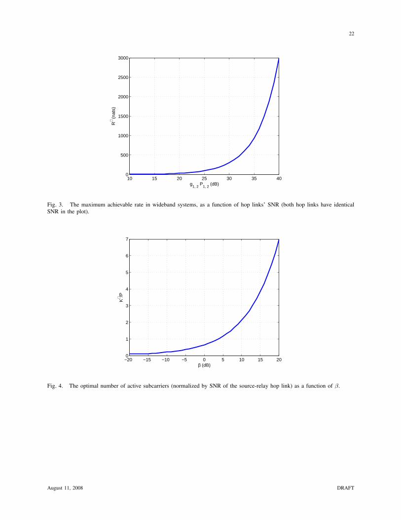
growth slope. To further elaborate on this issue, let g1P1 = P and g2P2 = βP , where β > 0 is
fixed as P changes. Now consider the performance metric
f(t)
P=
1
Pt· log
[(1 + Pt)(1 + βPt)
1 + (1 + β)Pt
],
which is the ratio between the achievable rate upon activating 1/t subcarriers and P , and can be
maximized by changing Pt (equivalent to changing K/P , the SNR-normalized number of active
subcarriers), for any given β. In Figure 4 we plot the relationship between K∗/P and β (in dB).
As can be seen, the optimal number of active subcarriers increases with β; for example, if β = 1
(0 dB), then it is optimal to activate approximately 0.7P subcarriers. In Figure 5 we further plot
the relationship between R∗/P and β (in dB). To verify our observation in Figure 3, we can
see that R∗/P ≈ 0.3 at β = 1. As β increases (i.e., the relay-destination hop link becomes less
August 11, 2008 DRAFT
15
noisy), R∗/P gradually approaches one, corresponding to the wideband DF capacity P . This is
because as β → ∞, the relay-destination link effectively vanishes, and the two-hop system is
reduced to a single-hop system with the source-relay link only.
VI. CONTINUOUS FREQUENCY-DOMAIN CHANNEL RESPONSE
In the previous sections, we focus on multicarrier channels with a fixed number of subcarriers.
In physical systems, a multicarrier channel is obtained from discretizing a continuous frequency-
domain channel response into a collection of discrete frequency bins over each of which the
frequency response is approximately “flat”. In this section, we therefore present the problem in
the limit of continuous frequency-domain channel responses, and analyze the behavior of the
low-complexity suboptimal algorithm in Section IV.
We start with a two-hop network in which each hop link is described by a continuous-time
real baseband channel [14], as
Ytm(t) = ht
m(t) ∗ Xtm(t) + Zt
m(t), (32)
where the superscript ·t indicates that the variables are in time, and the subscript ·m = 1, 2 denotes
the source-relay link or the relay-destination link, respectively. The additive noise process Ztm(t)
is white Gaussian, with one-sided power spectral density N0. The channel input process Xtm(t)
is linearly convolved with the channel impulse response htm(t), modeling a linear-filter channel.
As we take Fourier transform of Equation (32), we obtain the frequency-domain description of
the hop links
Ym(f) = hm(f)Xm(f) + Zm(f). (33)
The continuous frequency-domain channel response hm(f) is the Fourier transform of htm(t).
For the subsequent exposition, it is convenient to extend the ranking operator from vectors to
continuous functions, as given in the following definition.
Definition 4: For a measurable nonnegative real function g(f) over the positive real line
f ≥ 0, the ranking operator R is defined such that R ◦ g(f) is another measurable nonnegative
real function over the positive real line, denoted by gR(f), satisfying:
1) For each α ≥ 0, we have
µ ({f : g(f) ≤ α}) = µ({f : gR(f) ≤ α}
), (34)
where µ(·) denotes the Lebesgue measure on the real line.
August 11, 2008 DRAFT

16
2) For arbitrary 0 ≤ f1 < f2, we have
gR(f1) ≥ gR(f2). (35)
Intuitively, the ranking operator is used to “re-index” the frequencies such that the resulting
frequency-domain channel responses are monotonically decreasing with frequency. Consequently,
no further permutation is needed in any discretized multicarrier systems. For simplicity, we
assume that for each m = 1, 2, both am(f) = |hm(f)|2/N0 and aRm(f) are sufficiently smooth
with piecewise continuous derivatives.
Now as we discretize the frequency line into infinitesimal bins and perform multicarrier
modulation over them, the resulting rate maximization problem for frequency-domain non-
regenerative relaying can be formulated in the following form:
max
∫ ∞
0
log(1 + ρ(f))df, (36)
s.t.∫ ∞
0
γm(f)df = Pm, m = 1, 2, (37)
where the SNR density function ρ(f) is given by
ρ(f) =aR
1 (f)aR2 (f)γ1(f)γ2(f)
aR1 (f)γ1(f) + aR
2 (f)γ2(f) + 1. (38)
With sufficiently fine discretization, it is in principle possible to carry out the linear search
procedure in Section III to find out the optimal solution to Equation (36). In practice, however,
the computational complexity of such a procedure is expected to be still prohibitive. Here we turn
to analyzing the behavior of the low-complexity suboptimal algorithm as proposed in Section
IV, for which we can establish analytical results.
Following Section IV, for the ranked frequency-domain channel responses aRm(f), m = 1, 2,
we need to find out a cutoff frequency f > 0, such that the transmitted signals have strictly
positive power density below f , and do not contain any component beyond f . There exists a
maximum value for possible f , since if f is chosen too large, the waterfilling procedure would
enforce some frequency components below f to be zero. To determine the maximum possible
f , we note that for a valid f , we have
γm(f) =1
λm
− 1
aRm(f)
, m = 1, 2, and ∀0 ≤ f ≤ f , (39)
and ∫ f
0
γm(f)df = Pm, m = 1, 2. (40)
August 11, 2008 DRAFT

17
Hence λm, m = 1, 2, should satisfy
1
λm
=1
f
∫ f
0
1
aRm(f)
df +Pm
f. (41)
On the other hand, for each m = 1, 2, since aRm(f) is monotonically decreasing with f , we need
to have 1/λm ≥ 1/aRm(f) to ensure γm(f) > 0 for all f < f . Therefore the maximum possible
f is the lesser between the solutions of the two equations
1
f
∫ f
0
1
aRm(f)
df +Pm
f=
1
aRm(f)
, m = 1, 2. (42)
Let us denote the maximum possible f by fmax. For each cutoff frequency f ≤ fmax, the
achievable rate is
R(f) =
∫ f
0
[log
(aR
1 (f)
λ1
− 1
)+ log
(aR
2 (f)
λ2
− 1
)− log
(aR
1 (f)
λ1
+aR
2 (f)
λ2
− 1
)]df, (43)
where λm, m = 1, 2, are given by Equation (41). The maximum rate of the low-complexity
suboptimal algorithm is therefore max0≤f≤fmaxR(f).
VII. SIMULATION RESULTS
In this section, we study the performance of the algorithms presented in Sections III and IV,
via Monte Carlo simulations as a theoretical analysis appears elusive (except for certain special
cases as in Section V).
For each realization of the two-hop N -subcarrier system, we randomly generate the link
channel profile coefficients {am[n]}Nn=1, m = 1, 2. Specifically, these coefficients are generated as
the squared magnitudes of 2N independent and identically distributed (i.i.d.) circularly symmetric
complex Gaussian random variables with zero mean and unit variance. Therefore the {am[n]}Nn=1,
m = 1, 2, are a collection of i.i.d. exponentially distributed random variables, corresponding to
the standard Rayleigh fading model. Such a link model may be a suitable choice for wireless
transmission over rich-scattering propagation environments with abundant multipath and without
significant line-of-sight paths. Simulation results for other transmission systems can be similarly
generated and are not presented in this paper.
In simulation we compute the following end-to-end achievable rates for comparison.
1) The capacity of the two-hop transmission system, which is achieved by the DF scheme,
with the source and the relay performing waterfilling to optimally allocate power among
subcarriers. The resulting rates will be indicated by “DF” in plots.
August 11, 2008 DRAFT

18
2) The rate achieved by the conventional AF scheme, in which the power is uniformly
allocated among subcarriers for both the source-relay link and the relay-destination link.
The resulting rates will be indicated by “AF” in plots.
3) The rate achieved by the optimal algorithm in Section III. The resulting rates will be
indicated by “optimal algorithm” in plots.
4) The rate achieved by the low-complexity suboptimal algorithm in Section IV. The resulting
rates will be indicated by “suboptimal algorithm” in plots.
To get a qualitative view of the execution of the algorithms, we plot in Figure 6 the snapshot
corresponding to a particular channel realization sample with N = 16 and P1 = P2 = 20 dB.
The x-axis indicates the number of active subcarriers through the execution of algorithm, and
the y-axis correspondingly indicates the achieved rate Rk when the k strongest subcarriers are
activated. Comparing the curves for the optimal (curve with circles) and the suboptimal (curve
with squares) algorithms, we find that the performance of the two algorithms are fairly close.
Both algorithms show that the maximum rates are achieved when the number of active subcarriers
is ten, implying that it is not optimal to activate all the available subcarriers. In particular, for
the suboptimal algorithm, it is seen that the achievable rate actually decreases as k goes beyond
ten.
For comparison, the capacity (achieved by DF) and the AF achievable rate are indicated in
Figure 6 as well. Even for the relatively small number of subcarriers (N = 16), we observe that
the multicarrier relay processing does not lead to a large performance gain compared with the
conventional scalar AF scheme.
To futher quantify the small gap between the optimal algorithm and the low-complexity
suboptimal algorithm, we plot in Figure 7 the empirical histogram of the ratio between the
rates achieved by the two algorithms. Due to the slow execution of the optimal algorithm in
practice, we take N = 16, a relatively small number. The number of channel realizations is 300
in generating Figure 7. Surprisingly, we notice that most of the time the gap is less than two
percent within the optimal performance. This observation is quite noteworthy, especially given
the simplicity of the suboptimal algorithm.
We plot in Figure 8 the empirical cumulative distribution functions (CDF) of the achievable
rates, for a system with parameters of N = 16 and P1 = P2 = 20 dB. The number of channel
realizations is 300. Obviously the CDF of the capacity (achieved by DF) dominates those of the
other transmission strategies, while the CDF of the AF achievable rate is the most inferior. The
August 11, 2008 DRAFT
19
CDF of the optimal algorithm and the suboptimal algorithm virtually overlap with each other
without much noticeable difference, and lie between that of the capacity and that of the AF
achievable rate.
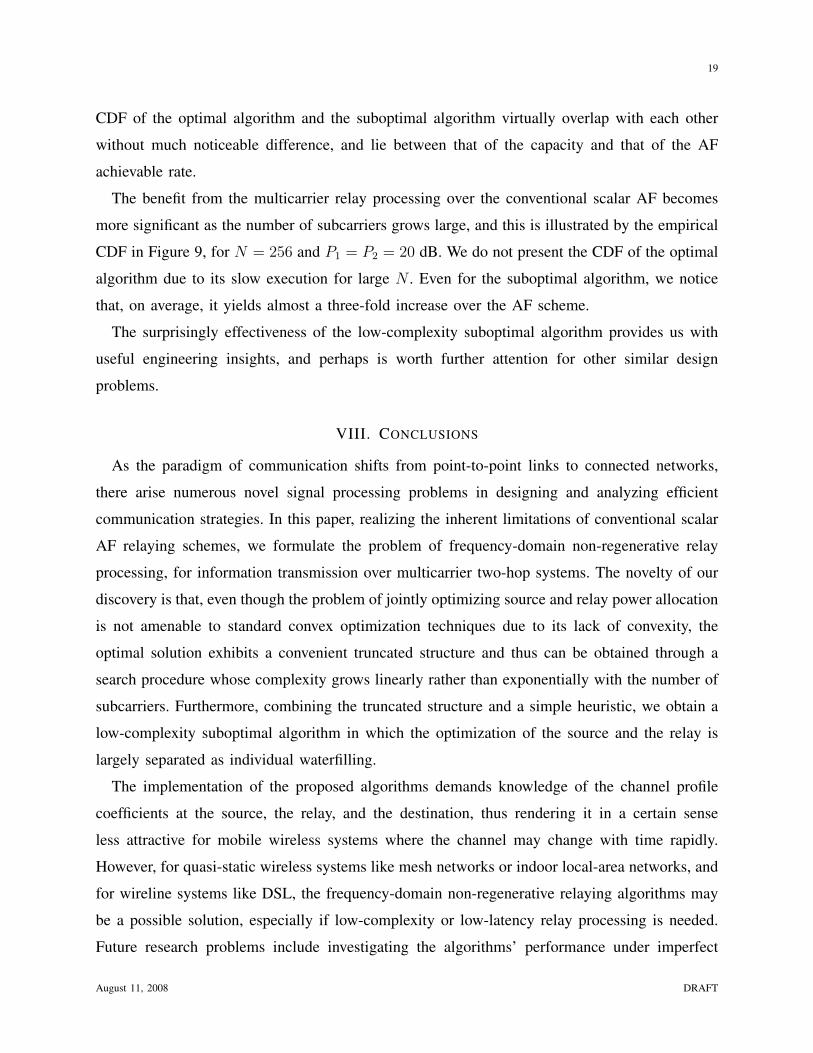
The benefit from the multicarrier relay processing over the conventional scalar AF becomes
more significant as the number of subcarriers grows large, and this is illustrated by the empirical
CDF in Figure 9, for N = 256 and P1 = P2 = 20 dB. We do not present the CDF of the optimal
algorithm due to its slow execution for large N . Even for the suboptimal algorithm, we notice
that, on average, it yields almost a three-fold increase over the AF scheme.
The surprisingly effectiveness of the low-complexity suboptimal algorithm provides us with
useful engineering insights, and perhaps is worth further attention for other similar design
problems.
VIII. CONCLUSIONS
As the paradigm of communication shifts from point-to-point links to connected networks,
there arise numerous novel signal processing problems in designing and analyzing efficient
communication strategies. In this paper, realizing the inherent limitations of conventional scalar
AF relaying schemes, we formulate the problem of frequency-domain non-regenerative relay
processing, for information transmission over multicarrier two-hop systems. The novelty of our
discovery is that, even though the problem of jointly optimizing source and relay power allocation
is not amenable to standard convex optimization techniques due to its lack of convexity, the
optimal solution exhibits a convenient truncated structure and thus can be obtained through a
search procedure whose complexity grows linearly rather than exponentially with the number of
subcarriers. Furthermore, combining the truncated structure and a simple heuristic, we obtain a
low-complexity suboptimal algorithm in which the optimization of the source and the relay is
largely separated as individual waterfilling.
The implementation of the proposed algorithms demands knowledge of the channel profile
coefficients at the source, the relay, and the destination, thus rendering it in a certain sense
less attractive for mobile wireless systems where the channel may change with time rapidly.
However, for quasi-static wireless systems like mesh networks or indoor local-area networks, and
for wireline systems like DSL, the frequency-domain non-regenerative relaying algorithms may
be a possible solution, especially if low-complexity or low-latency relay processing is needed.
Future research problems include investigating the algorithms’ performance under imperfect
August 11, 2008 DRAFT

20
channel knowledge, extending the problem and its algorithms to multihop transmission systems
with more than two hops, and combining the problem with interference mitigation in DSL
systems.
ACKNOWLEDGMENT
The authors wish to thank Prof. Yingbo Hua of University of California Riverside and Mr.
Xiaojun Tang of Rutgers University for helpful discussion.
REFERENCES
[1] W. Zhang and U. Mitra, “Channel-Adaptive Frequency-Domain Relay Processing in Multicarrier Multihop Transmission,”
in Proc. IEEE International Conference on Acoustic, Speech, and Signal Processing (ICASSP), Las Vegas, NV, Mar.-Apr.
2008.
[2] M. Haenggi and D. Puccinelli, “Routing in Ad Hoc Networks: A Case for Long Hops,” IEEE Communication Magazine,
Vol. 43, No. 10, pp. 93-101, Oct. 2005.
[3] M. Sikora, J. N. Laneman, M. Haenggi, D. J. Costello, Jr., and T. E. Fuja, “Bandwidth- and Power-Efficient Routing in
Linear Wireless Networks,” IEEE Trans. Inform. Theory, Vol. 52, No. 6, pp. 2624-2633, Jun. 2006.
[4] U. Niesen, C. Fragouli, and D. Tuninetti, “Scaling Laws for Line Networks: From Zero-Error to Min-Cut Capacity,” in
Proc. IEEE International Symposium on Information Theory (ISIT), Seattle, WA, Jul. 2006.
[5] O. Oyman and S. Sandhu, “Non-Ergodic Power-Bandwidth Tradeoff in Linear Multi-hop Networks,” in Proc. IEEE
International Symposium on Information Theory (ISIT), Seattle, WA, Jul. 2006.
[6] W. Zhang and U. Mitra, “Multihopping Strategies: An Error-Exponent Comparison,” in Proc. IEEE International Symposium
on Information Theory (ISIT), Nice, France, Jun. 2007.
[7] E. C. Posner and A. L. Rubin, “The Capacity of Digital Links in Tandem,” IEEE Trans. Inform. Theory, Vol. 30, No. 3,
pp. 464-470, May 1984.
[8] T. M. Cover and J. A. Thomas, Elements of Information Theory, John Wiley & Sons, Inc., New York, 1991.
[9] S. Boyd and L. Vandenberghe, Convex Optimization, Cambridge University Press, 2004.
[10] X. Tang and Y. Hua, “Optimal Design of Non-Regenerative MIMO Wireless Relays,” IEEE Trans. Wireless Commun.,
Vol. 6, No. 4, pp. 1398-1407, Apr. 2007.
[11] Z. Fang, Y. Hua, and J. C. Koshy, “Joint Source and Relay Optimization for a Non-Regenerative MIMO Relay,” in Proc.
IEEE Workshop on Sensor Array and Multi-channel Processing, Waltham, MA, Jul. 2006.
[12] D. G. Brennan, “Linear Diversity Combining Techniques,” Proc. IRE, Vol. 47, No. 1, pp. 1075-1102, Jun. 1959.
[13] R. Cendrillon, J. Huang, M. Chiang, and M. Moonen, “Autonomous Spectrum Balancing for Digital Subscriber Lines,”
IEEE Trans. Signal Process., Vol. 55, No. 8, pp. 4241-4257, Aug. 2007.
[14] G. D. Forney, Jr. and G. Ungerboeck, “Modulation and Coding for Linear Gaussian Channels,” IEEE Trans. Inform.
Theory, Vol. 44, No. 6, pp. 2384-2415, Oct. 1998.
[Authors’ Bio]
August 11, 2008 DRAFT

21
Fig. 1. Schematic illustration of the relay processing. Note that the additional standard multicarrier modulation/demodulationsteps, viz., adding/removing cyclic prefix and parallel/serial conversions are not explicitly displayed.
10 15 20 25 30 35 4010
0
101
102
103
104
g1, 2
P1, 2
(dB)
K∗ ≈
1/t∗
Fig. 2. The optimal number of subcarriers in wideband systems, as a function of hop links’ SNR (both hop links have identicalSNR in the plot).
August 11, 2008 DRAFT
22
10 15 20 25 30 35 400
500
1000
1500
2000
2500
3000
g1, 2
P1, 2
(dB)
R∗ (
nats
)
Fig. 3. The maximum achievable rate in wideband systems, as a function of hop links’ SNR (both hop links have identicalSNR in the plot).
−20 −15 −10 −5 0 5 10 15 200
1
2
3
4
5
6
7
β (dB)
K∗ /P
Fig. 4. The optimal number of active subcarriers (normalized by SNR of the source-relay hop link) as a function of β.
August 11, 2008 DRAFT

23
−20 −15 −10 −5 0 5 10 15 200
0.1
0.2
0.3
0.4
0.5
0.6
0.7
0.8
0.9
β (dB)
R∗ /P
Fig. 5. The maximum achievable rate (normalized by SNR of the source-relay hop link) as a function of β.
0 2 4 6 8 10 12 14 165
10
15
20
25
30
k (# of active subcarriers)
Rat
e (n
ats)
DF
AF
optimal algorithm
suboptimal algorithm
optimal # ofactivesubcarriers
Fig. 6. The snapshot of the execution of the algorithms, corresponding to a particular channel realization sample. The systemparameters are N = 16, P1 = P2 = 20 dB.
August 11, 2008 DRAFT

24
95.5 96 96.5 97 97.5 98 98.5 99 99.5 1000
0.02
0.04
0.06
0.08
0.1
0.12
0.14
R/R∗ (%)
Pro
babi
lity
Fig. 7. The empirical histogram of the ratio between the rates achieved by the suboptimal algorithm and the optimal algorithm.The system parameters are N = 16, P1 = P2 = 20 dB. The number of channel realizations is 300.
10 15 20 25 30 350
0.1
0.2
0.3
0.4
0.5
0.6
0.7
0.8
0.9
1
R (nats)
Pr[
Rat
e ≤
R]
DF
AF
optimalalgorithm
suboptimalalgorithm
Fig. 8. The empirical CDF of the achievable rates. The system parameters are N = 16, P1 = P2 = 20 dB. The number ofchannel realizations is 300.
August 11, 2008 DRAFT

25
0 20 40 60 80 100 1200
0.1
0.2
0.3
0.4
0.5
0.6
0.7
0.8
0.9
1
R (nats)
Pr[
Rat
e ≤
R]
AFsuboptimalalgorithm DF
Fig. 9. The empirical CDF of the achievable rates. The system parameters are N = 256, P1 = P2 = 20 dB. The number ofchannel realizations is 300.
August 11, 2008 DRAFT