Embed Size (px)
Citation preview

Optimal Portfolio Strategy for Risk Management in Toll Road Forecasts and Investments 1
2 3
Rohan Shah* 4 Analyst and Task Manager 5
CDM Smith Inc. 6 Toll Finance and Technology Group 7
12357-A Riata Trace Parkway, Suite 210 8 Austin, TX 78727 9
Phone: 1-512-992-7350 10 Email: [email protected] 11
12 Phani Jammalamadaka 13
Associate and Local Team Leader 14 CDM Smith Inc. 15
Toll Finance and Technology Group 16 2301 Maitland Center Parkway, Suite 300 17
Maitland, FL 32751 18 Phone: 1-407-618-1921 19
Email: [email protected] 20 21 22
*Corresponding Author 23 24 25
Submitted for presentation and publication at the 26 96th Annual Meeting of the Transportation Research Board 27
January 2017, Washington D.C. 28 29
30
31
32
Word count: 33 Text: 6774 words 34 Tables: 0 × 250 = 0 word equivalents 35 Figures: 4 × 250 = 1000 word equivalents 36 Total: 7774 words 37 38 39 Original submission: August 1, 2016 40
Revised submission: November 15, 2016 41
42 43 44 45 46

Shah and Jammalamadaka
2
ABSTRACT 1
The study leverages modern portfolio theory and stochastic time series models to develop a new risk 2
management strategy for future traffic projections along brownfield toll facilities. Uncertainty in future 3
traffic forecasts may give rise to concerns about performance reliability and revenue potential. Historical 4
time series of traffic data offered by brownfield corridors are utilized for developing econometric forecast 5
estimates, and Monte-Carlo simulation is used to quantify à priori risks or variance in them. Optimal 6
forecast portfolios are developed using mean-variance optimization strategies. Numerical analysis is 7
presented using historical toll transactions along the Massachusetts Turnpike system. Suggested 8
diversification strategies are found to achieve better forecast efficiencies in the long-term, with better 9
tradeoffs between expected returns and risks. Forecast performance expectations and risk-propensity of 10
planners and agencies are thus jointly captured. 11
Keywords: modern portfolio theory; risk management; Monte-Carlo simulation; traffic and toll revenue 12
studies; stochastic time series, mean-variance optimization 13
14
15
16
17
18
19
20
21
22
23
24
25
26
27
28
29
30
31

Shah and Jammalamadaka
3
1 BACKGROUND AND STUDY APPROACH 1
1.1 Toll Road Forecasting and Financing under À Priori Uncertainty 2
Transportation infrastructure and tolling industry are witnessing a variety of project financing, 3
procurement, and delivery methods such as design-build, build-operate-transfer, public-private 4
partnerships, and concessionaires. Such alternative mechanisms often help meet financing gaps 5
considering limited federal budgets. They are also sensitive to uncertainty and risks surrounding long-6
term performance and profitability. Toll road assets are generally part of revenue-dependent infrastructure 7
systems that rely on traffic across the facility for revenue generation, return on investments, debt 8
coverage, and operations and maintenance costs. 9
That being said, natural concerns often surround the reliability of any prediction or forecasting activity in 10
general. Such concerns originate from intrinsic uncertainty about the future, and in the case of toll 11
facilities, several exogenous factors such as market volatility and future economic growth. They often 12
pose challenges in long-range toll network planning and policymaking, and also in determining financial 13
feasibility due to unpredictable future cash flows. Reliability of forecasted toll returns is also affected by 14
operational factors like potential revenue ‘leakage’ from unaccounted transactions (especially in toll 15
charging methods involving video/picture-capture of license plates, and pay-by-mail setups), and 16
incomplete recovery of tariffs and fines from toll violators. In recent times, varying user-adoption levels 17
of widespread conversion to electronic toll collection (ETC) systems also pose a challenge in estimating 18
their true market penetration and revenue yield. Jammalamadaka et al. (2013) provide further insight into 19
sources of T&R uncertainty from both supply and demand-side perspectives. Bain (2009) presents a 20 synthesis of potential errors and biases in traffic forecasts. Additional studies highlighting T&R forecast 21
uncertainty include Lemp and Kockelman (2009), and Flyvbjerg et al. (2005) who identify differences in 22
forecasted and actual traffic patterns along not just toll roads but also other existing transportation 23
systems including public transit. Toll infrastructure practices are thus often confronted with traffic 24
forecasting and investment decision-making under various kinds of à priori uncertainties. This warrants 25
robust and strategic approaches for proactive risk or uncertainty management, which is the underlying 26
motivation of this study. 27
1.2 Optimal Portfolio-based Risk Management 28
From a broader perspective, this study postulates that the aforementioned challenges of T&R forecasting 29
and investment under uncertainty have parallels with monetary investments in stock markets, real assets 30
and even commodities which are also sensitive to market trends and volatility. This is an attempt to link 31
T&R forecasting and toll road investment workflows with financial investment strategies for real assets. 32
Specifically, it leverages strategies from the modern portfolio theory (MPT) originally proposed by 33 Markowitz (1952). MPT provides a set of effective tools widely applied in finance, markets, and 34
investment economics. Qualitatively, it suggests diversification among all available investment assets or 35
options with a view to spread out the risks. Quantitatively, it enables optimal asset allocation by 36
constructing portfolios to optimize or maximize expected returns based on their prevalent risks. Risk 37
represents the likelihood of the returns increasing or diminishing in value and by how much, and hence 38
represented by variance or standard deviation of the rate of return. Higher expected returns inherently 39
carry higher risks. MPT also incorporates the correlation and covariance between assets, in order to 40
capture their variation relative to each other. It also assumes ‘rational’ investor behavior, where they want 41
to minimize their risks. However, investors willing to rake in additional risk also expect to be 42
compensated with higher expected returns. 43

Shah and Jammalamadaka
4
In the same spirit, an array of available forecast models is treated as assets or options available to 1
planners, which is also a hypothetical portfolio of sorts. Planners are also faced with a decision to choose 2
the ‘best’ forecast estimates. Along the lines of investment portfolios developed in financial MPT, this 3
study proposes a notion of ‘forecast portfolio’ which contains the set of forecast options or models to 4
choose from. For the purpose of analysis, time series-based forecast models are used in this study. 5
However, they can be replaced by any stochastic forecasting tools available to practitioners. Each model 6
option projects their own set of forecasts, which are equivalent to expected returns. However due to the 7
presence of future uncertainty and risks, they are equivalents of risky assets. A practical challenge arises 8
in quantifying risks or variance from model forecasts. In this study, standard deviation or variance in 9
forecasts is used to quantify risks. Expected values (or returns) and variance (or risks) in forecasts from 10
each model contribute to returns and risks of the combined forecast portfolio. 11
An optimal forecast portfolio provides a forecast value derived using an optimal combination of multiple 12
forecast options, as opposed to a singular, undiversified forecast estimate. In line with merits of MPT 13
strategies, optimal allocations of investments and forecast expectations across individual forecast assets in 14
the portfolio can collectively manage risks more effectively. They can also better inform financing 15
decisions that significantly depend on expected forecast projections. The allocation or diversification 16
across forecast assets each of which has a unique combination of risk and return can also be case-specific. 17
In other words, it can be tailored according to preferred degrees of risk-averseness or risk-affinity of the 18
concessionaire, tolling agencies or financers, and in certain cases even project or system-specific 19
conditions. 20
1.3 Study Applicability and Contributions 21
The current study leverages econometric time series tools to develop the various forecast options 22
comprising the portfolio. Two independent classes of univariate time series models are estimated, 23
including Autoregressive Integrated Moving Average (ARIMA), and Brownian Motion Mean Reversion 24
(BMMR) models. Each has unique mathematical properties and forecasting structures. Econometric time 25
series models for any variable typically build on historical data and past trends, and hence the 26
applicability of the current study also relies on historical toll transactions data over existing toll facilities. 27
Accordingly, application of the current approach and framework is suitable for existing open facilities 28
with rich historical data. These models learn discernable patterns in input data and previous growth rate 29
trends, and are adaptive to any extreme events (such as a major economic recession, like the one in 2008) 30
that may be reflected from data movements in the past. The risk analysis workflow includes Monte-Carlo 31
simulation-based techniques that quantify the variance in forecast estimates. Monte-Carlo techniques not 32
only help evaluate relative risk levels of each model forecasts but also identify the largest contributors to 33
the overall risk of the forecast portfolio. Use of Monte-Carlo methods for risk analysis in revenue-based 34
infrastructure and road investments can also be found in Songer et al. (1997) and Lam and Tam (1998) 35
respectively. Wibowo and Kochendörfer (2005) use Latin Hypercube simulation for financial risk 36
analysis in the context of Indonesian toll roads. Simulation-based techniques have earlier been found to 37
provide effective and computationally tractable approaches to risk analysis. The current study extends the 38
literature by using them to quantify uncertainty in the context of univariate time series model forecasts for 39
toll traffic. 40
The study contributions span across both academic research and industry. It can be used to jointly manage 41
forecast expectations and risks, and can be used to assist policies and decision-making to mitigate the 42
effects of uncertainty. The study also leverages well-known economic strategies of MPT to propose a 43
novel risk management approach to fit toll T&R forecasting. From the practice standpoint, single-point 44

Shah and Jammalamadaka
5
forecasts from demand-model based T&R studies or forecast streams developed through other means can 1
be overlaid with probabilistic streams from stochastic time series models. This can help develop an early 2
understanding of à priori risks associated with long-term traffic forecasts and toll revenue potential. 3
These can also be engaged to proactively plan for risks, and design more adaptive toll policies. Forecast 4
risks are also linked with concerns about financial returns on infrastructure investments, future toll policy 5
development, and long-term toll network expansion. Comprehensive long-range T&R studies in toll 6
industry practice typically use a travel demand-toll diversion modeling framework for forecasting. The 7
methods presented in this paper can be used to supplement and cross-check the forecasts developed in 8
traditional long-range T&R forecast studies. 9
The tolling industry and practice thus face ever-growing needs of new analytical methods and policies for 10
forecast risk management. The current study develops one such set of workable tools. They are designed 11
to leverage several interdisciplinary strategies also with a view to make them versatile and conceivable 12
enough to the diverse mix of stakeholders involved. 13
2 TOLL TRANSACTIONS FORECASTING USING TIME SERIES MODELS 14
Annual transactions are considered in this study to avoid any seasonality effects in data. The subsections 15
below describe the models, cover brief numerical experiments that validate their predicted forecasts over 16
observed field data, and produce long-term forecasts. Several studies have demonstrated applications of 17
the time series models in traffic predictions, including Nihan and Holmesland (1980), Williams (2001), 18
Williams and Hoel (2003), and Ghosh et al. (2009). 19
2.1 Model Descriptions 20
2.1.1 ARIMA Model 21
ARIMA is a combination of an autoregressive (AR) and a moving average (MA) models. The term 22
‘integrated’ represents additional operations to stationarize the data. Stationarity of a time series variable 23
indicates that its mean and variance do not change with time, and this can often be achieved using 24
differencing operations. AR components indicate dependence of a variable on its own prior values. It is 25
conceivable from practical experience and has been demonstrated in studies that traffic patterns in urban 26
corridors evolve over time and have interdependencies with their past patterns. This notion is extended to 27
toll transactions in the same spirit here. MA components model prediction error of the independent 28
variable as a function of its own past errors, again a practically perceivable notion in practice where 29
forecast errors may accumulate and propagate through time. 30
ARIMA models are specified as ARIMA(p,d,q), where arguments p,d,q represent the orders of the AR, 31
differencing, and MA components respectively. Qualitatively p and q also indicate number of historical 32
data lags and forecast error terms affecting the present value. For the current study dataset, individual 33
correlation effects are found to be insignificant beyond the first order lags, and thus higher-order models 34
are not found to be good fits to data. First-order model specifications such as ARIMA(1,1,0), 35
ARIMA(0,1,1) and ARIMA(1,1,1) are thus estimated on the differenced dataset. For the purpose of 36
comparison and expanding the diversity of the forecast portfolio, additional second-order specifications 37
including ARIMA(0,1,2) and ARIMA(2,1,0) are also estimated. 38
The forecasting operation under ARIMA is conducted by taking the expectation of the time series, or 39
expected values of transactions and error terms. This can also be referred to as deterministic forecasting. 40
Under this case, the error terms are eliminated since their expected values are zero. 41

Shah and Jammalamadaka
6
2.1.2 BMMR Model 1
BMMR models are part of the broader class of Brownian motion (BM) models. BM models are more 2
commonly applied in financial economics to study patterns of particularly volatile or dynamic market 3
variables such as stocks, commodity or asset prices, and interest rates, as found in Osborne (1962), and 4
Dixit and Pindyick (1994), among others. Previous applications in the transportation/traffic forecasting 5
domain have been limited, such as in some studies including Soliño et al. (2012), Galera and Soliño 6
(2010). Their application is also recently validated in Shah and Jammalamadaka (2016). 7
The sub-class of mean reverting models (BMMR) is driven by a mean-reversion process which is used for 8
modeling financial assets and commodities or generally quantities where an infinite growth is not 9
practically possible. 10
2.1.3 Risk Analysis and Monte-Carlo Simulation Framework 11
Both the time series models used in this study have stochastic elements in the form of ‘error terms’ that 12
are present at every stage of forecasting. Error terms qualitatively indicate likely deviation of forecasts 13
from actual values if available, or expected values if estimating or forecasting. They are random variables 14
representing both the uncertain magnitudes and unpredictable trends of these deviations. Even though 15 their ‘expected value’ is statistically zero (so they disappear under deterministic forecasting), under 16
realistic conditions where forecasts are produced they may take finite measurable values. 17
As part of the risk analysis approach in this study, stochasticity is introduced using a Monte-Carlo 18
simulation of these error terms. It includes random sampling of the error terms that helps assign 19 confidence bands around the single-point forecasts produced deterministically. The theoretical basis for 20
this approach is that the randomness associated with every model forecast arises from the error term 𝑒𝑡, 21
which follows a Gaussian (Normal) distribution as follows: 𝑒𝑡~𝑖. 𝑖. 𝑑. 𝒩(0, 𝜎2). These error terms thus 22 sampled from a Gaussian distribution give a range of errors and subsequently forecast estimates (in the 23
form of confidence bounds). The risk analysis approach thus treats the forecast estimates as random 24
variables themselves. Further mathematical description of error sampling can be found in the literature on 25
theoretical time series, such as Box et al. (1994), and Enders (1995). 26
Extending the forecasting approach into a stochastic framework also allows for consideration of 27
sensitivities of forecasts to market volatility and uncertainty in growth rate projections. It provides a 28
means to test the robustness of the process by simulating a range of mathematically possible forecasts at 29
any given time-step, and capture the expected variance. 30
2.2 Empirical Validation 31
A case study of the Massachusetts Turnpike corridor is used as a test-bed application of the proposed 32
method. Historical system-wide toll transactions data dating back to 1950s are acquired. Model validation 33
tests for the two time series forecast models are thus conducted on real observed transaction data on the 34
study facilities. A fraction of the original data is kept aside exclusively for this purpose and not used 35
during model estimation (hence also called ‘out-of-sample testing’). Four years’ worth of annual 36
transactions data (from 2010-2013) are used for validation, and the mean absolute percentage error 37
(MAPE) is used to quantify the prediction accuracy. The MAPE is a measure of accuracy of any 38
forecasting method and is defined by the formula: 39

Shah and Jammalamadaka
7
𝑀𝐴𝑃𝐸 =1
𝑁(∑ |
𝑥𝑖 − 𝑥�̂�
𝑥𝑖| ∗ 100
𝑁
𝑖=1
) (1) 1
where, 2
{𝑥𝑖} = actual observations of the time series 3
{𝑥�̂�} = the estimated or forecasted time series 4
𝑁 = number of non-missing data points 5
The validation results, including comparison with the actual transactions and the MAPE calculations are 6
summarized in Figures 1(a) and 1(b) respectively below. 7
The models are also mobilized for forecasting into the long-term future, under a 30-year future planning 8
horizon (through 2040). Planning and programming decisions regarding toll roads or their expansions are 9
generally long-term. They are also fiscally aligned with regional transportation or thoroughfare 10
improvements dictated in long-range transportation plans for the area. Various degrees of confidence 11
intervals (5%, 25%, 75%, 95%) are obtained, along with expected values of forecasts. However, for ease 12 of representation in the plot area, they are plotted only for the preferred model specification (one with the 13
lowest MAPE during the forecast validation tests). Forecast streams are illustrated below in Figure 1(c). 14
It can be seen that the long-range forecast streams are a reflection of the validation period, indicating a 15
mix of forecast performance by the models in the portfolio, ranging from conservative, neutral, to 16
aggressive forecasts. Confidence intervals for only the preferred model specification are illustrated. It is 17
worth noting that expected value forecast paths from all other models lie within a 5%-75% bands of the 18
preferred specification. These confidence intervals can qualitatively help visualize a ‘best-case/worst-19
case’ outlook for forecasts. Under the various upper and lower confidence bounds of the expected value 20
forecast path, a wide range of possible future deviations away from the expected values (due to 21
uncertainty and unknown future market factors) are expected to lie. 22

Shah and Jammalamadaka
8
1 (a) Short term forecasts: Comparison with actuals 2
3
4
(b) Empirical validation: Mean absolute prediction errors 5
60
62
64
66
68
70
72
74
76
78
80
2010 2011 2012 2013
An
nu
al T
ota
l Tra
nsa
ctio
ns
Mill
ion
s
Forecast Model Validation Year
Observed ARIMA(0,1,1) ARIMA(1,1,1) ARIMA(1,1,0)
ARIMA(2,1,0) BMMR ARIMA(1,0,1)
0
1
2
3
4
5
6
ARIMA(0,1,1) ARIMA(1,1,1) ARIMA(1,1,0) ARIMA(2,1,0) BMMR ARIMA(1,0,1)
MA
PE
(%)
Forecast Assets (Models)

Shah and Jammalamadaka
9
1
(c) Long-term forecasts: expected values and confidence intervals 2
FIGURE 1 Toll transactions forecast streams using various time series model options 3
It can be seen that the selected time series models each predict a unique set of forecasts. The 4
ARIMA(0,1,1) specification and the BMMR model each have good empirical fit and the smallest range of 5
prediction errors (≤ 1%). The other first-order specifications ARIMA(1,0,1) and ARIMA(1,1,0) have 6 slightly higher but acceptable MAPE ranges. However the second-order specification ARIMA(2,1,0) 7
specification appears to have the highest MAPE range among these candidate models, and its forecasts 8
over the validation period also appear to be higher, and thus more on the aggressive side. 9
The forecast portfolio composition for the case-study is quite diverse, and contains a good mix of 10
aggressive and conservative model assets. 11
3 FORECAST PORTFOLIOS 12
3.1 Forecast Portfolio Risk and Return 13
Monte-Carlo simulation of transactions forecasts projected by the time-series models above provides a 14
range of possible forecast options and help quantify expected returns and risks associated with each. They 15
also help identify individual options contributing most to the overall portfolio risks. As in the time series 16
models, forecasts of transactions are thus treated as random variables. Expected forecast returns in a 17
particular year are computed using the expected value of the probability distribution of forecasts, and 18
forecast risk is measured by the estimated variance or standard deviation around the expected value in the 19
distribution. Gaussian distributions of transactions are assumed in this study, as they are a function of the 20
distribution of the error terms in the underlying time series models as discussed earlier. In essence, 21
transactions forecasts are thus treated as random variables, with an expected value and variance of 22
projections in every year along the future planning horizon. 23
In line with assumptions of MPT, it is assumed that planners or agencies are generally risk-averse with 24
regard to forecasts, meaning that given two portfolios that offer the same forecast returns (or expected 25
values of forecast projections), the less risky one (with lesser variance) is more likely to be preferred. 26
Investors are sometimes willing to take on additional risk if compensated by higher expected returns, and 27

Shah and Jammalamadaka
10
conversely, investors targeting higher expected returns must accept more risk. In a similar spirit, more 1
optimistic forecast performance expectations or more aggressive revenue projections come with higher 2
risks or higher portfolio variance. The resulting trade-off between forecasting returns and risks achieved 3
from portfolio optimization is the same for all project stakeholders. Different parties, however, can 4
evaluate the trade-off differently based on their independent risk preferences. It is thus important to 5
quantify combined portfolio risks and returns, as opposed to respective values of the individual forecast 6
options. 7
For a general case of 𝑛 individual forecast options or models 𝑖, let 𝑟𝑖 denote the returns or forecast 8
projections from each of them, and 𝐸(𝑟𝑖) its expected value. Thus given this set of risky options, a set of 9
weights 𝑊 describing the optimal distribution of a forecast portfolio of size 𝑛 is defined. It is the 10
proportion in which the overall portfolio is split among the individual model options. Let 𝑤𝑖 be the 11
optimal weight for an option 𝑖, which also indicates the proportion of the overall forecast returns to be 12
assigned to model i. All weights are also assumed to be non-negative. 13
The returns from the overall forecast portfolio containing the above forecast assets is denoted by 𝑟𝑝, and 14
the portfolio return’s expected value is computed by the following vector combination of individual 15
options: 16
𝐸(𝑟𝑝) = ∑ 𝑤𝑖𝐸(𝑟𝑖)
𝑛
𝑖=1
(2) 17
The sum of optimal weights across individual options is equal to one, shown by: 18
∑ 𝑤𝑖 = 1
𝑛
𝑖=1
(3) 19
The portfolio return computation thus involves finding the weighted average return of the individual 20
components. Portfolio variance 𝜎𝑝2, (or standard deviation 𝜎𝑝
) on the other hand, is defined in terms of 21
both individual variance of options and also the expected variability among all component asset pairs 22
(𝑖, 𝑗) or the forecasted covariance. Let an estimate of the covariance matrix of individual options be 23
represented by Σp. The overall risks of a portfolio of forecast options is thus equal to the weighted 24
average covariance of the individual forecast returns, denoted as follows in the scalar notation: 25
𝑉𝑎𝑟(𝑟𝑝) = 𝜎𝑝2 = ∑ ∑
𝑛
𝑗=1
𝑤𝑖𝑤𝑗𝐶𝑜𝑣(𝑟𝑖, 𝑟𝑗)
𝑛
𝑖=1
(4) 26
Covariance can also be expressed in terms of the correlation coefficient 𝜌𝑖𝑗 between the returns from a 27
pair of forecasts options (𝑖, 𝑗), and standard deviations of individual assets, 𝜎𝑖 and 𝜎𝑗 as follows: 28
𝐶𝑜𝑣(𝑟𝑖, 𝑟𝑗) = 𝜌𝑖𝑗𝜎𝑖𝜎𝑗 (5) 29
The portfolio variance can thus also be expressed in terms of the correlation coefficient as follows: 30
𝑉𝑎𝑟(𝑟𝑝) = ∑ ∑
𝑛
𝑗=1
𝑤𝑖𝑤𝑗𝜌𝑖𝑗𝜎𝑖𝜎𝑗
𝑛
𝑖=1
(6) 31

Shah and Jammalamadaka
11
A weight vector 𝒘 is an 𝑛-dimensional vector that represents the weight assignment across individual 1
forecast options in a given portfolio containing 𝑛 assets. Portfolio variance can be represented in the 2
vector notation as: 3
𝑉𝑎𝑟(𝑟𝑝) = 𝒘 𝐓. Σp. 𝒘 (7) 4
In summary, the estimate of the expected return for each forecast option or model is its average value 5
across the range of forecasts in a particular planning year. The estimate of variance is the average value of 6
the squared deviations around the forecast mean, and the estimate of covariance is the average value of 7
the cross-product of deviations across the different forecast options under consideration. When the 8
options are combined into a forecast portfolio, the expected value and variance of the portfolio 9
accommodates both an individual option’s properties and the covariance among the available options. 10
3.2 Mean-Variance Optimization Strategies 11
This subsection discusses the model formulations for a few standard classes of portfolio optimization 12
methods. For the current study, five different optimization models each with a different policy goal are 13
formulated. They are developed for a general 𝑛-options (or 𝑛-forecast model) portfolio. All the models 14 are part of the broader mean-variance optimization (MVO) class of models that aim to jointly optimize 15
expected values and variance of a variable. 16
3.2.1 Global Minimum Forecast Portfolio Variance (Global MFPV) 17
MFPV is a constrained minimization problem that seeks to minimize the overall risk of the forecast 18
portfolio subject to basic constrains related to weight on an individual forecast option 𝑤𝑖. This particular 19 formulation is called ‘global’ MFPV since there are no conditions or expectations tied around the overall 20
forecast returns from the portfolio, as long as the portfolio variance or risks are minimum. The 21
formulation is developed as follows: 22
min𝑤∈𝑊
𝜎𝑝 (8) 23
subject to: 24
∑ 𝑤𝑖 = 1
𝑛
𝑖=1
(9) 25
𝑤𝑖 ≥ 0 ∀ 𝑖 ∈ (1, 𝑛) (10) 26
27
The first constraint indicates that the individual weights must sum to one, and the second is the non-28
negativity constraint that indicates all the weights must be non-negative. The solution to this model is 29
trivial, as the selection merely involves choosing the model with the minimum observed variance. 30
3.2.2 MFPV with Target Forecast Returns 31
This is very similar to the Global MFPV formulation, but with additional expectations regarding the 32
forecast returns. This model addresses a dual objective of maximum forecast returns and minimum 33
forecast risks. Consider the following optimization formulation: 34

Shah and Jammalamadaka
12
min𝑤∈𝑊
𝜎𝑝 (11) 1
subject to: 2
∑ 𝑤𝑖 = 1
𝑛
𝑖=1
(12) 3
𝑤𝑖 ≥ 0 ∀ 𝑖 ∈ (1, 𝑛) (13) 4
𝐸(𝑟𝑝) ≥ max(𝐸(𝑟𝑖)) ∀ 𝑖 ∈ (1, 𝑛) (14) 5
As seen from the model formulation, this model has an additional third constraint requiring the forecast 6
portfolio returns to be greater than the best possible returns from all individual model assets. 7
3.2.3 Global Maximum Forecast Portfolio Returns (Global MFPR) 8
This model is the dual of the Global MFPV model formulation. It is also a single objective optimization 9
problem, aiming on maximizing forecast returns from the portfolio without limitations on the additional 10
risks accumulated alongside. The formulation is as follows: 11
max𝑤∈𝑊
𝐸(𝑟𝑝) (15) 12
subject to: 13
∑ 𝑤𝑖 = 1
𝑛
𝑖=1
(16) 14
𝑤𝑖 ≥ 0 ∀ 𝑖 ∈ (1, 𝑛) (17) 15
The solution to this model is also trivial, as one can just select the forecast asset that projects the 16 maximum forecast returns and assign the maximum weight (or rather the entire portfolio weight) to it. It 17 must be noted however that high returns also contain high risks, and under most practical applications the 18 objectives may be to minimize overall variance as opposed to singularly maximizing returns. 19 20 3.2.4 MFPR with Target Forecast Variance 21
This model is similar to the Global MFPR model but with an additional constraint related to the forecast 22
variance. This model attempts to maximize the forecast returns from the portfolio but is concerned with 23
the additional risks, and thus tries to limit the variance at the lowest possible variance across individual 24
options (or target variance). The formulation for this case is as follows: 25
max𝑤∈𝑊
𝐸(𝑟𝑝) (18) 26
subject to: 27
∑ 𝑤𝑖 = 1
𝑛
𝑖=1
(19) 28
𝑤𝑖 ≥ 0 ∀ 𝑖 ∈ (1, 𝑛) (20) 29
𝜎𝑝 ≤ min(𝜎𝑖
) ∀ 𝑖 ∈ (1, 𝑛) (21) 30
Shah and Jammalamadaka
13
The last expression is the target minimum portfolio variance constraint. 1
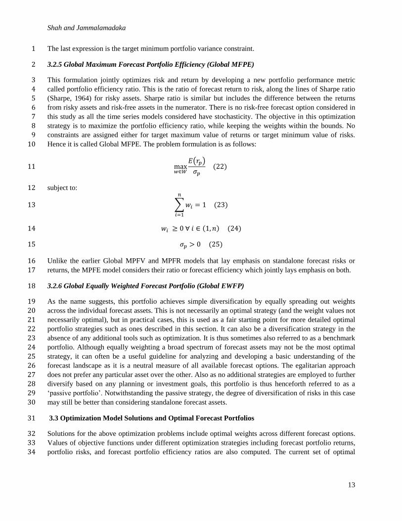
3.2.5 Global Maximum Forecast Portfolio Efficiency (Global MFPE) 2
This formulation jointly optimizes risk and return by developing a new portfolio performance metric 3
called portfolio efficiency ratio. This is the ratio of forecast return to risk, along the lines of Sharpe ratio 4
(Sharpe, 1964) for risky assets. Sharpe ratio is similar but includes the difference between the returns 5
from risky assets and risk-free assets in the numerator. There is no risk-free forecast option considered in 6
this study as all the time series models considered have stochasticity. The objective in this optimization 7
strategy is to maximize the portfolio efficiency ratio, while keeping the weights within the bounds. No 8
constraints are assigned either for target maximum value of returns or target minimum value of risks. 9
Hence it is called Global MFPE. The problem formulation is as follows: 10
max𝑤∈𝑊
𝐸(𝑟𝑝)
𝜎𝑝 (22) 11
subject to: 12
∑ 𝑤𝑖 = 1
𝑛
𝑖=1
(23) 13
𝑤𝑖 ≥ 0 ∀ 𝑖 ∈ (1, 𝑛) (24) 14
𝜎𝑝 > 0 (25) 15
Unlike the earlier Global MPFV and MPFR models that lay emphasis on standalone forecast risks or 16
returns, the MPFE model considers their ratio or forecast efficiency which jointly lays emphasis on both. 17
3.2.6 Global Equally Weighted Forecast Portfolio (Global EWFP) 18
As the name suggests, this portfolio achieves simple diversification by equally spreading out weights 19
across the individual forecast assets. This is not necessarily an optimal strategy (and the weight values not 20
necessarily optimal), but in practical cases, this is used as a fair starting point for more detailed optimal 21
portfolio strategies such as ones described in this section. It can also be a diversification strategy in the 22
absence of any additional tools such as optimization. It is thus sometimes also referred to as a benchmark 23
portfolio. Although equally weighting a broad spectrum of forecast assets may not be the most optimal 24
strategy, it can often be a useful guideline for analyzing and developing a basic understanding of the 25
forecast landscape as it is a neutral measure of all available forecast options. The egalitarian approach 26
does not prefer any particular asset over the other. Also as no additional strategies are employed to further 27
diversify based on any planning or investment goals, this portfolio is thus henceforth referred to as a 28
‘passive portfolio’. Notwithstanding the passive strategy, the degree of diversification of risks in this case 29
may still be better than considering standalone forecast assets. 30
3.3 Optimization Model Solutions and Optimal Forecast Portfolios 31
Solutions for the above optimization problems include optimal weights across different forecast options. 32
Values of objective functions under different optimization strategies including forecast portfolio returns, 33
portfolio risks, and forecast portfolio efficiency ratios are also computed. The current set of optimal 34
Shah and Jammalamadaka
14
portfolios is developed for a future planning year 2020. This is only for demonstration and the framework 1
is generic and can be applied for any future year of interest. 2
The efficacy of the diversification strategy over selection of standalone forecast options can also be 3
quantified. Risks and returns yielded by the several combinations of optimal portfolios (including the 4
passive portfolio) are compared with those from the individual model options. Essential characteristics of 5
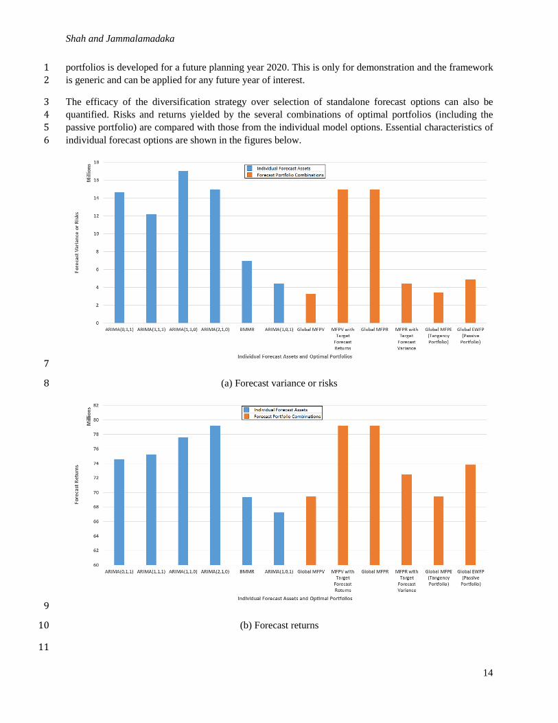
individual forecast options are shown in the figures below. 6
7
(a) Forecast variance or risks 8
9
(b) Forecast returns 10
11

Shah and Jammalamadaka
15
1
(c) Forecast efficiency ratio 2
FIGURE 2 Performance metrics for individual forecast options and combined forecast portfolios 3
Forecast variance for returns projected by individual model assets, their expected returns, and efficiency 4
ratios are plotted in Figures 2(a), (b), and (c) respectively. Forecast returns from the Global MFPR and 5
MFPV with Target Forecast Returns strategies are found to correspond with the highest possible returns 6
projected by individual forecast assets. However, forecast risks or variance under the risk-averse 7
strategies including Global MFPV, MFPR with Target Forecast Variance, and the efficiency oriented 8
Global MFPE strategy are found with lower forecast risks than those carried by all individual forecast 9
assets. Also forecast efficiency ratios achieved under these three strategies are found to be higher than 10
efficiencies under all individual forecast assets. Apart from the optimal portfolio strategies, the Global 11
EWFP strategy which suggests a passive portfolio with equal weight allocation also underscores the 12
merits of diversification. The portfolio variance for the passive portfolio is found to be lower than almost 13
all individual assets in both case studies, and forecast efficiency ratios found to be higher. Thus overall, 14
portfolio optimization strategies and diversifications are generally found to outperform the individual 15
forecast assets in terms of risk optimization and achieving better efficiency ratios. 16
Results for the optimal weight assignments across the different forecast options are shown below. These 17
weights hold under the current estimates of individual forecast returns, variance, and covariance. Results 18
for all the five MVO-classes of strategies are shown, but ones for the passive portfolio strategy are not 19
shown since it is nothing but an equal weight assignment. 20

Shah and Jammalamadaka
16
1
FIGURE 3 Weight allocations across forecast options under optimal portfolio strategies 2
It can be seen that for the first case-study application, the Global MFPV, MFPR with Target Forecast 3
Variance, and Global MFPE models suggest diversification across individual forecast assets, but not the 4
models with the Global MFPR and MFPV with Target Forecast Returns strategies. Both the latter models 5
are inclined towards maximizing forecast returns, and the optimization models find that assigning 6
maximum (or rather the entire) weightage on the asset providing the highest returns in both cases, or the 7
ARIMA(2,1,0) model provides the highest overall portfolio returns. Recollect however, that this is a 8
trivial solution from the Global MFPR strategy and doesn’t result in a diversified portfolio. As mentioned 9
earlier, this can generally be a most risky proposition, and in simple terms, amounts to “putting all eggs in 10
one basket”. Other strategies result in relatively more diversified portfolios. The Global MFPV strategy, 11
as expected, suggests the comparatively highest allocation on a model with the lowest variance, which is 12
ARIMA(1,0,1). Also the optimal weight for this model is almost thrice that of the second preferred model 13
which is BMMR. For the MFPR with Target Forecast Variance strategy, a higher weight is assigned to 14
the BMMR model than the ARIMA(1,0,1) model, though the corresponding weights are not much 15
different. The Global MFPE strategy also results in the ARIMA(1,0,1) model getting the highest 16
weightage followed by the BMMR. 17
Asset weights in optimal portfolios are found to be driven by the respective individual asset 18
characteristics such as their expected returns, variance and forecast efficiency. It is worth noting that these 19
optimal weights, naturally, are sensitive to the current optimization model formulations and constraints. 20
Relaxation of any constraint on the decision variables, particularly the non-negativity of may result in 21
different optimal combinations, but that aspect is not explored in the current study. 22
5 RECOMMENDATIONS FOR RISK MANAGEMENT 23
This section develops policy and practice takeaways from the current study approach and the findings 24
from the case-study application. 25
0
0.2
0.4
0.6
0.8
1
1.2
Global MFPV MFPV with TargetForecast Returns
Global MFPR MFPR with TargetForecast Variance
Global MFPE
Op
tim
al F
ore
cast
Ass
et
(Mo
de
l) W
eig
hts
Forecast Portfolio Optimization Strategy
ARIMA(0,1,1) ARIMA(1,1,1) ARIMA(1,1,0) ARIMA(2,1,0) BMMR ARIMA(1,0,1)
Shah and Jammalamadaka
17
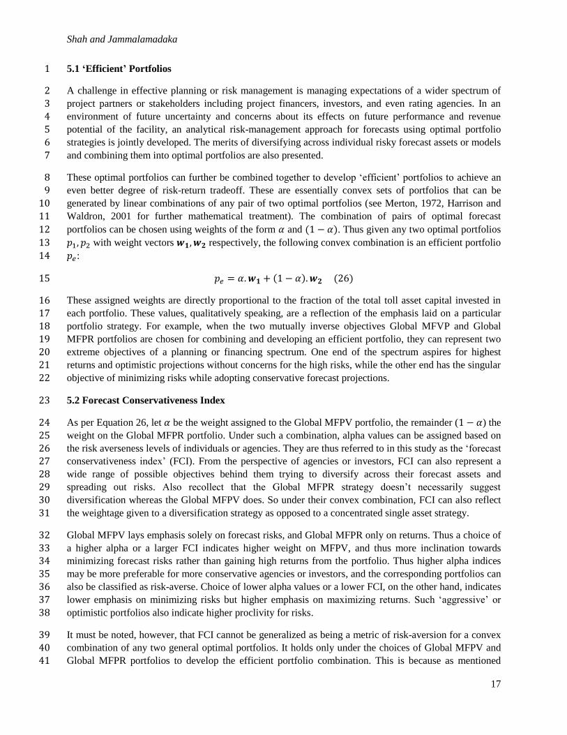
5.1 ‘Efficient’ Portfolios 1
A challenge in effective planning or risk management is managing expectations of a wider spectrum of 2
project partners or stakeholders including project financers, investors, and even rating agencies. In an 3
environment of future uncertainty and concerns about its effects on future performance and revenue 4
potential of the facility, an analytical risk-management approach for forecasts using optimal portfolio 5
strategies is jointly developed. The merits of diversifying across individual risky forecast assets or models 6
and combining them into optimal portfolios are also presented. 7
These optimal portfolios can further be combined together to develop ‘efficient’ portfolios to achieve an 8
even better degree of risk-return tradeoff. These are essentially convex sets of portfolios that can be 9
generated by linear combinations of any pair of two optimal portfolios (see Merton, 1972, Harrison and 10
Waldron, 2001 for further mathematical treatment). The combination of pairs of optimal forecast 11
portfolios can be chosen using weights of the form 𝛼 and (1 − 𝛼). Thus given any two optimal portfolios 12
𝑝1 , 𝑝2
with weight vectors 𝒘𝟏, 𝒘𝟐 respectively, the following convex combination is an efficient portfolio 13
𝑝𝑒 : 14
𝑝𝑒 = 𝛼. 𝒘𝟏 + (1 − 𝛼). 𝒘𝟐 (26) 15
These assigned weights are directly proportional to the fraction of the total toll asset capital invested in 16
each portfolio. These values, qualitatively speaking, are a reflection of the emphasis laid on a particular 17
portfolio strategy. For example, when the two mutually inverse objectives Global MFVP and Global 18
MFPR portfolios are chosen for combining and developing an efficient portfolio, they can represent two 19
extreme objectives of a planning or financing spectrum. One end of the spectrum aspires for highest 20
returns and optimistic projections without concerns for the high risks, while the other end has the singular 21
objective of minimizing risks while adopting conservative forecast projections. 22
5.2 Forecast Conservativeness Index 23
As per Equation 26, let 𝛼 be the weight assigned to the Global MFPV portfolio, the remainder (1 − 𝛼) the 24
weight on the Global MFPR portfolio. Under such a combination, alpha values can be assigned based on 25
the risk averseness levels of individuals or agencies. They are thus referred to in this study as the ‘forecast 26 conservativeness index’ (FCI). From the perspective of agencies or investors, FCI can also represent a 27
wide range of possible objectives behind them trying to diversify across their forecast assets and 28
spreading out risks. Also recollect that the Global MFPR strategy doesn’t necessarily suggest 29
diversification whereas the Global MFPV does. So under their convex combination, FCI can also reflect 30
the weightage given to a diversification strategy as opposed to a concentrated single asset strategy. 31
Global MFPV lays emphasis solely on forecast risks, and Global MFPR only on returns. Thus a choice of 32
a higher alpha or a larger FCI indicates higher weight on MFPV, and thus more inclination towards 33
minimizing forecast risks rather than gaining high returns from the portfolio. Thus higher alpha indices 34
may be more preferable for more conservative agencies or investors, and the corresponding portfolios can 35
also be classified as risk-averse. Choice of lower alpha values or a lower FCI, on the other hand, indicates 36
lower emphasis on minimizing risks but higher emphasis on maximizing returns. Such ‘aggressive’ or 37
optimistic portfolios also indicate higher proclivity for risks. 38
It must be noted, however, that FCI cannot be generalized as being a metric of risk-aversion for a convex 39 combination of any two general optimal portfolios. It holds only under the choices of Global MFPV and 40
Global MFPR portfolios to develop the efficient portfolio combination. This is because as mentioned 41

Shah and Jammalamadaka
18
earlier, these are two inverse portfolios with one focusing unequivocally only on risks and the other only 1
on returns. Their combination thus represents polarized objectives of minimizing forecast risks and 2
maximizing forecast returns, and the relative degree of each captured through FCI. 3
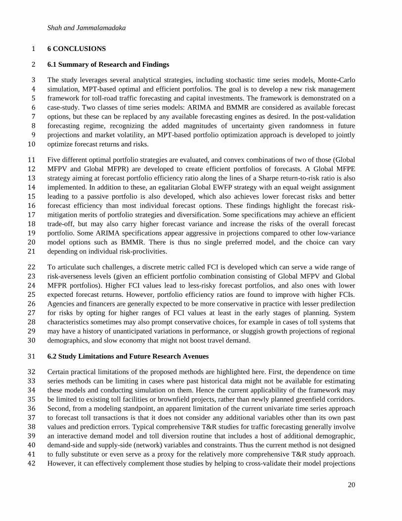
The effects of selection of a range of FCI values on forecast returns, risks, and also the forecast efficiency 4
ratio of the forecast portfolio are demonstrated in the figures below. 5
6 (a) Forecast portfolio variance or risks 7
8
9 (b) Forecast portfolio returns 10

Shah and Jammalamadaka
19
1 (c) Forecast portfolio efficiency ratios 2
FIGURE 4 Forecast conservativeness indices and portfolio characteristics 3
4
As seen from the trends, increasing FCI indicates a higher degree of forecast risk-averseness. Also 5
consistent with those objectives, the forecast variance or risk levels are found to decrease. In line with 6
basic characteristics of any common financial portfolio produced using MPT, the forecast portfolios 7
developed in this study indicate that forecast returns at lower risk levels are also low in proportion. This 8
trend can again be observed in the trends of decreasing forecast returns with increasing conservativeness 9
or FCI. The third set of plots indicates the forecast portfolio efficiency ratios improve with higher values 10
of FCI, which can be attributed to a drop in forecast variance. 11
5.3 Role of System-Specific Characteristics 12
Apart from risk-averseness preferences, system characteristics such as operations may also play a role in 13
selecting ranges of the FCI. For the purposes of long-range planning and toll infrastructure programming, 14
toll network planners and bidders in coordination with local agencies can adopt FCI ranges based on their 15
understanding of what fits the respective system best. Governmental support or assurance on investment 16
returns may also promote optimism among bidders and contractors, an example being a guaranteed level 17
of minimum revenue that is designed to alleviate the concern of demand risk (Cheah and Liu, 2005). Toll 18
facilities in developing areas with modest projections of traffic and demographic growth in the near future 19
might prompt selection of more conservative forecasts (higher FCI values). Inversely, low-variance 20
forecasts or high-growth facilities might create more room for taking risks. It may prompt adoption of 21
relatively aggressive forecast portfolios (lower ranges of FCI values). 22
More often though, or in the absence of any conspicuous system characteristics, planning decisions tend 23
to gravitate towards the low to moderate risk category, and as found here, this can also help improve 24
forecast portfolio efficiency in trying to achieve an optimal risk-return trade-off. Agencies can also design 25 future toll schedules and plan toll rate revisions based on the expected forecast returns on transactions and 26
the corresponding risk levels in a way that favorable revenue streams are generated in the future. 27
28
Shah and Jammalamadaka
20
6 CONCLUSIONS 1
6.1 Summary of Research and Findings 2
The study leverages several analytical strategies, including stochastic time series models, Monte-Carlo 3
simulation, MPT-based optimal and efficient portfolios. The goal is to develop a new risk management 4
framework for toll-road traffic forecasting and capital investments. The framework is demonstrated on a 5
case-study. Two classes of time series models: ARIMA and BMMR are considered as available forecast 6
options, but these can be replaced by any available forecasting engines as desired. In the post-validation 7
forecasting regime, recognizing the added magnitudes of uncertainty given randomness in future 8
projections and market volatility, an MPT-based portfolio optimization approach is developed to jointly 9
optimize forecast returns and risks. 10
Five different optimal portfolio strategies are evaluated, and convex combinations of two of those (Global 11
MFPV and Global MFPR) are developed to create efficient portfolios of forecasts. A Global MFPE 12
strategy aiming at forecast portfolio efficiency ratio along the lines of a Sharpe return-to-risk ratio is also 13
implemented. In addition to these, an egalitarian Global EWFP strategy with an equal weight assignment 14
leading to a passive portfolio is also developed, which also achieves lower forecast risks and better 15
forecast efficiency than most individual forecast options. These findings highlight the forecast risk-16
mitigation merits of portfolio strategies and diversification. Some specifications may achieve an efficient 17
trade-off, but may also carry higher forecast variance and increase the risks of the overall forecast 18
portfolio. Some ARIMA specifications appear aggressive in projections compared to other low-variance 19
model options such as BMMR. There is thus no single preferred model, and the choice can vary 20
depending on individual risk-proclivities. 21
To articulate such challenges, a discrete metric called FCI is developed which can serve a wide range of 22
risk-averseness levels (given an efficient portfolio combination consisting of Global MFPV and Global 23
MFPR portfolios). Higher FCI values lead to less-risky forecast portfolios, and also ones with lower 24
expected forecast returns. However, portfolio efficiency ratios are found to improve with higher FCIs. 25
Agencies and financers are generally expected to be more conservative in practice with lesser predilection 26 for risks by opting for higher ranges of FCI values at least in the early stages of planning. System 27
characteristics sometimes may also prompt conservative choices, for example in cases of toll systems that 28
may have a history of unanticipated variations in performance, or sluggish growth projections of regional 29
demographics, and slow economy that might not boost travel demand. 30
6.2 Study Limitations and Future Research Avenues 31
Certain practical limitations of the proposed methods are highlighted here. First, the dependence on time 32
series methods can be limiting in cases where past historical data might not be available for estimating 33
these models and conducting simulation on them. Hence the current applicability of the framework may 34
be limited to existing toll facilities or brownfield projects, rather than newly planned greenfield corridors. 35
Second, from a modeling standpoint, an apparent limitation of the current univariate time series approach 36
to forecast toll transactions is that it does not consider any additional variables other than its own past 37
values and prediction errors. Typical comprehensive T&R studies for traffic forecasting generally involve 38
an interactive demand model and toll diversion routine that includes a host of additional demographic, 39
demand-side and supply-side (network) variables and constraints. Thus the current method is not designed 40
to fully substitute or even serve as a proxy for the relatively more comprehensive T&R study approach. 41
However, it can effectively complement those studies by helping to cross-validate their model projections 42
Shah and Jammalamadaka
21
and quantify potential forecast risk. In combination with conventional four-step demand models, these 1
methods can help to improve forecast reliability and make better planning and investment decisions. 2
These limitations open the avenues for several continuing and future research possibilities. Multivariate 3
time series models that consider additional supply-side variables or historical demographic trends are 4
worth exploring, as are more advanced time series models such as the Generalized Autoregressive 5
Conditional Heteroskedasticity (GARCH). On the financial-side, given that the asset investment 6
landscape changes quite dynamically and as newer infrastructure financing and risk-sharing instruments 7 such as public-private partnerships emerge rapidly in urban toll road projects, planners or investors may 8
not always conform to the rationality assumptions of the MPT such as inherent risk-averseness. 9
Additional insights may be borrowed from behavioral finance to design assorted portfolios, and more 10
innovative portfolio optimization strategies for toll road assets. 11
REFERENCES 12
1. Adler, T., Doherty, M., Klodzinski, J., & Tillman, R. (2014). Methods for Quantitative Risk Analysis 13
for Travel Demand Model Forecasts. Transportation Research Record: Journal of the Transportation 14
Research Board, No. 2429, 1-7. 15
2. Bain, R. (2009). Error and optimism bias in toll road traffic forecasts. Transportation, 36(5), 469-482. 16
3. Box, G. E. P., G. M. Jenkins, and G. C. Reinsel. (1994) Time Series Analysis: Forecasting and 17
Control 3rd ed. Englewood Cliffs, NJ, Prentice Hall. 18
4. Cheah, C. Y., and Liu, J. (2006). Valuing governmental support in infrastructure projects as real 19 options using Monte Carlo simulation. Construction Management and Economics, 24(5), 545-554. 20 21
5. Dixit, A. K., & Pindyck, R. S. (1994). Investment under uncertainty. Princeton University Press 22
6. Enders, W. (1995) Applied Econometric Time Series. Hoboken, NJ: John Wiley & Sons. 23
7. Flyvbjerg, B., M. K. S. Holm, and S. L. Buhl (2005). How (In)Accurate Are Demand Forecasts in 24
Public Works Projects? The Case of Transportation. Journal of the American Planning Association, 25
71(2), 131–146. 26
8. Galera, A. L. L., & Soliño, A. S. (2010). A real options approach for the valuation of highway 27
concessions. Transportation Science, 44(3), 416-427 28
29
9. Ghosh, B., Basu, B., & O'Mahony, M. (2009). Multivariate short-term traffic flow forecasting using 30
time-series analysis. IEEE Transactions on Intelligent Transportation Systems, 10(2), 246-254. 31
10. Harrison, M., & Waldron, P. (2011). Mathematics for economics and finance. Routledge. 32
11. Jammalamadaka P., Jarmarwala Y., Hirunyanitiwattana W., & Mokkapati N., (2013), Comparative 33
Analysis of Traffic and Revenue Risks Associated with Priced Facilities, 14th TRB National 34
Transportation Planning Applications Conference, Presentation 332. 35
12. Lam, W. H., & Tam, M. L. (1998). Risk analysis of traffic and revenue forecasts for road investment 36
projects. Journal of Infrastructure Systems, 4(1), 19-27. 37
Shah and Jammalamadaka
22
13. Laughton, D. G., & Jacoby, H. D. (1995). The effects of reversion on commodity projects of different 1
length. Real options in capital investments: Models, strategies, and applications. Ed. by L. Trigeorgis. 2
Westport: Praeger Publisher, 185-205 3
14. Lemp, J. D., and Kockelman K.M. Understanding and Accommodating Risk and Uncertainty in Toll 4
Road Projects: A Review of the Literature. In Transportation Research Record: Journal of the 5
Transportation Research Board, No. 2132, 106–112. 6
15. Markowitz, H. (1952). Portfolio selection. The Journal of Finance, 7(1), 77-91. 7
16. Massachusetts Turnpike Information Center (2013). 8
https://www.massdot.state.ma.us/Portals/0/docs/infoCenter/financials/toll_reports/YearlyTrafficReve9
nue2013.pdf 10
17. Nihan, N. L., & Holmesland, K. O. (1980). Use of the Box and Jenkins time series technique in traffic 11
forecasting. Transportation, 9(2), 125-143. 12
18. Merton, R. C. (1972). An analytic derivation of the efficient portfolio frontier. Journal of Financial 13
and Quantitative Analysis, 7(04), 1851-1872. 14
19. Osborne, M. F. M. (1962). Periodic structure in the Brownian motion of stock prices. Operations 15
Research, 10(3), 345-379. 16
20. Panayiotou, A., & Medda, F. (2016). Portfolio of Infrastructure Investments: Analysis of European 17
Infrastructure. Journal of Infrastructure Systems (2016), 04016011 18
21. Shah R., Jammalamadaka P. (2016). Brownian Motion Models for Toll Traffic Forecasting and 19
Financing Strategies under Uncertainty, TRB 95th Annual Meeting Compendium of Papers, 20
Washington, D.C. Paper No. 16-6708. 21
22. Sharpe, W. F. (1964). Capital asset prices: A theory of market equilibrium under conditions of risk, 22
Journal of Finance, 19 (3), 425-442. 23
23. Soliño, A.S., Galera, A.L.L., & Lorenzo, A. (2012). Unit Root Analysis of Traffic Time Series in Toll 24
Highways. Journal of Civil Engineering and Architecture, 6(12), 1641-164 25
24. Songer, A. D., Diekmann, J., & Pecsok, R. S. (1997). Risk analysis for revenue dependent 26
infrastructure projects. Construction Management & Economics, 15(4), 377-382. 27
25. Wibowo, A., & Kochendörfer, B. (2005). Financial risk analysis of project finance in Indonesian toll 28
roads. Journal of Construction Engineering and Management, 131(9), 963-972. 29
26. Williams, B. M. (2001). Multivariate vehicular traffic flow prediction: Evaluation of ARIMAX 30
modeling. Transportation Research Record 1776, Transportation Research Board, Washington, D.C., 31
194–200. 32
27. Williams, B. M., & Hoel, L. A. (2003). Modeling and forecasting vehicular traffic flow as a seasonal 33 ARIMA process: Theoretical basis and empirical results. Journal of transportation engineering, 34
129(6), 664-672. 35
36