Embed Size (px)
Citation preview

arX
iv:1
910.
0096
8v2
[cs
.IT
] 4
Feb
202
11
On the Optimality of Reconfigurable Intelligent
Surfaces (RISs): Passive Beamforming,
Modulation, and Resource Allocation
Minchae Jung, Member, IEEE, Walid Saad, Fellow, IEEE,
Merouane Debbah, Fellow, IEEE, and Choong Seon Hong, Senior Member, IEEE
Abstract
Reconfigurable intelligent surfaces (RISs) have recently emerged as a promising technology that
can achieve high spectrum and energy efficiency for future wireless networks by integrating a massive
number of low-cost and passive reflecting elements. An RIS can manipulate the properties of an incident
wave, such as the frequency, amplitude, and phase, and, then, reflect this manipulated wave to a desired
destination, without the need for complex signal processing. In this paper, the asymptotic optimality
of achievable rate in a downlink RIS system is analyzed under a practical RIS environment with its
associated limitations. In particular, a passive beamformer that can achieve the asymptotic optimal
performance by controlling the incident wave properties is designed, under a limited RIS control link
and practical reflection coefficients. In order to increase the achievable system sum-rate, a modulation
scheme that can be used in an RIS without interfering with existing users is proposed and its average
symbol error rate is asymptotically derived. Moreover, a new resource allocation algorithm that jointly
considers user scheduling and power control is designed, under consideration of the proposed passive
beamforming and modulation schemes. Simulation results show that the proposed schemes are in close
agreement with their upper bounds in presence of a large number of RIS reflecting elements thereby
verifying that the achievable rate in practical RISs satisfies the asymptotic optimality.
M. Jung is with the Department of Electronic Engineering, Soonchunhyang University, Asan, Chungcheongnam-do, Rep. of
Korea (e-mail: [email protected]).
W. Saad is with Wireless@VT, Department of Electrical and Computer Engineering, Virginia Tech, Blacksburg, VA 24061
USA (e-mail: [email protected]).
M. Debbah is with CentraleSupelec, Universite Paris-Saclay, 91192 Gifsur-Yvette, France and Mathematical &
Algorithmic Sciences Lab, Huawei Technologies France SASU, 92100 Boulogne-Billancourt, France (e-mail: mer-
C. Hong is with the Department of Computer Science and Engineering, Kyung Hee University, Yongin-si, Gyeonggi-do 17104,
Rep. of Korea (e-mail: [email protected]).

2
Index Terms
Reconfigurable intelligent surface (RIS), metasurface, passive beamforming, resource allocation,
I. INTRODUCTION
The concept of a metasurface is rapidly emerging as a key solution to support the demand for
massive connectivity, mainly driven by upcoming Internet of Things (IoT) and 6G applications
[1]–[19]. A metasurface relies on a massive integration of artificial meta-atoms that are commonly
made of metal structures of low-cost and passive elements [20], [21]. Each meta-atom can
manipulate the incident electromagnetic (EM) wave impinging on it, in terms of frequency,
amplitude, and phase, and reflect it to a desired destination, without additional signal processing.
A metasurface can potentially provide reliable and pervasive wireless connectivity given that
man-made structures, such as buildings, walls, and roads, can be equipped with metasurfaces in
the near future and used for wireless transmission [4]–[6]. Moreover, a tunable metasurface can
significantly enhance the signal quality at a receiver by allowing a dynamic manipulation of the
incident EM wave. Tunable metasurfaces are mainly controlled by electrical, optical, mechanical,
and fluid operations [7] that can be programmed in software using a field programmable gate
array (FPGA) [8]. The concept of a reconfigurable intelligent surface (RIS) is essentially an
electronically operated metasurface controlled by programmable software, as introduced in [7]
and [8]. In wireless communication systems, a base station (BS) can send control signals to
an RIS controller (i.e., FPGA) via a dedicated control link and controls the properties of the
incident wave to enhance the signal quality at the receiver. In principle, the electrical size of the
unit reflecting elements (i.e., meta-atoms) deployed on RIS is between λ/8 and λ/4, where λ
is a wavelength of radio frequency (RF) signal [7]. Note that conventional large antenna-array
systems, such as a massive multiple-input and multiple-output (MIMO) and MIMO relay system,
typically require antenna spacing of greater than λ/2 [5]. Therefore, an RIS can provide more
reliable and space-intensive communications compared to conventional antenna-array systems as
clearly explained in [4]–[6]. Therefore, a large number of reflecting elements can be arranged on
each RIS thus offering precise control of the reflection wave and allowing it to coherently align
with the desired channel. Furthermore, an RIS can be used with other promising communication
techniques, such as simultaneous wireless information and power transfer (SWIPT) [22], [23]
and physical layer security [24]. Hence, the use of RIS has been recognized as a promising
technology for future 6G wireless systems [25]–[27].

3
A. Related Works
Owing to these advantages, the use of an RIS in wireless communication systems has recently
received significant attention as in [1] and [8]–[14]. An RIS is typically used for two main
wireless communication purposes: a) RIS as an RF chain-free transmitter and b) RIS as a
passive beamformer that amplifies the incident waveform (received from a BS) and reflects it to
the desired user, so-called as intelligent reflecting surface (IRS). In [8], the authors analyzed the
error rate performance of a phase-shift keying (PSK) signaling and proved that an RIS transmitter
equipped with a large number of reflecting elements can convey information with high reliability.
The works in [9] and [10] proposed RF chain-free transmitter architectures enabled by an RIS
that can support PSK and quadrature amplitude modulation (QAM). Meanwhile, the works in [1]
and [11] designed joint active and passive beamformer that minimize the transmit power at the
BS, under discrete and continuous phase shifts, respectively. Also, in [12] and [13], the authors
designed a passive beamformer that maximizes the ergodic data rate and the energy efficiency,
respectively. Moreover, the work in [8] theoretically analyzed the average symbol error rate (SER)
resulting from an ideal passive beamformer and proved that the SER decays exponentially as the
number of reflecting elements on RIS increases. In [14], we provided a first insight on a passive
beamformer that can achieve, asymptotically, an ideal RIS performance. However, these previous
studies in [1] and [8]–[14] have not considered practical RIS environments and their limitations,
such as practical reflection coefficients and the limited capacity of the RIS control link. In fact,
an RIS can manipulate the properties of an incident wave based on the resonant frequency of the
tunable reflecting circuit. Then, the incident EM power is partially consumed at the resistance
of the reflecting circuit according to the difference between the incident wave frequency and the
resonant frequency. This results in the amplitude of the reflection coefficients less than or equal
to one depending on the phase shifts of the incident wave. However, the works in [1], [8], [11]
and [12] assumed an ideal RIS whose amplitude of the reflection coefficients are always equal
to one which is impractical for an RIS. Moreover, in [8] and [11]–[14], the authors assumed a
continuous phase shift at each reflecting element. However, this continuous phase shift requires
infinite bits to control each reflecting element and the RIS control link between a BS and an RIS
cannot support those infinite control bits. Finally, the signals from the RIS transmitters proposed
in [9] and [10] can be undesired interference for existing cellular network, given that those RISs

4
operate as an underlay coexistence with cellular networks. Therefore, there is a need for new
analysis of practical RISs when dealing with a limited RIS control link capacity and practical
reflection coefficients that can verify the asymptotic optimality of realistic RISs.
B. Contributions
The main contribution of this paper is a rigorous optimality analysis of the data rates that
can be achieved by an RIS under consideration of practical reflection coefficients with a limited
RIS control link capacity1. In this regard, we first design a passive beamformer that achieves
asymptotic signal-to-noise ratio (SNR) optimality, regardless of the reflection power loss and
the number of RIS control bits. In particular, the proposed passive beamformer with one bit
RIS control can achieve the asymptotic SNR of an ideal RIS with infinite control bits, lead to
a much simpler operation at the BS especially for a large number of reflecting elements on an
RIS. We then propose a new modulation scheme that can be used in an RIS to achieve sum-rate
higher than the one achieved by a conventional network without RIS. In the proposed modulation
scheme, each RIS utilizes an ambient RF signal, convert it into desired signal by controlling
the properties of incident wave, and transmit it to the desired user, without interfering with
existing users. We also prove that the achievable SNR from the proposed modulation converges
to the asymptotic SNR resulting from a conventional massive MIMO or MIMO relay system,
as the number of reflecting elements on an RIS increases. Given the aforementioned passive
beamformer and modulation scheme, we finally develop a novel resource allocation algorithm
whose goal is to maximize the average sum-rate under the minimum rate requirements at each
user. We then study, analytically, the potential of an RIS by showing that a practical RIS can
achieve the asymptotic performance of an ideal RIS, as the number of RIS reflecting elements
increases without bound. Our simulations show that the proposed schemes can asymptotically
achieve the performance resulting from an ideal RIS and its upper bound.
The rest of this paper is organized as follows. Section II describes the system model. Section
III describes the optimality of achievable rate in downlink RIS system. Simulation results are
provided in Section IV to support and verify the analyses, and Section V concludes the paper.
Notations: Throughout this paper, boldface upper- and lower-case symbols represent matrices
1An asymptotic optimal performance can be achieved by an ideal RIS which has infinite and continuous phase shifts and
lossless reflection coefficients and is higher than that of a massive MIMO system as proved in [1].

5
Fig. 1. Illustrative system model of the considered RIS-based MISO system.
and vectors respectively, and IM is a size-M identity matrix. (A)i,j refers to an element at row
i and column j of a matrix A The conjugate, transpose, and Hermitian transpose operators are
(·)∗, (·)T, and (·)H, respectively. The norm of a vector a is ‖a‖, the amplitude and phase of
a complex number a are denoted by |a| and ∠a, respectively. E [·], Var [·], and Cov [·] denote
expectation, variance, and covariance operators, respectively. O(·) denotes the big O notation
and CN (m, σ2) denotes a complex Gaussian distribution with mean m and variance σ2.
II. SYSTEM MODEL
Consider a single BS multiple-input single-output (MISO) system that consists of a set K of
K single-antenna user equipments (UEs) and multiple RISs each of which having N reflecting
elements, as shown in Fig. 1. The BS is equipped with M antennas and serves one UE at
each resource block (RB) based on an orthogonal frequency-division multiple-access (OFDMA)
scheme. We assume that the total system bandwidth is equally divided into C orthogonal subcar-
riers and F orthogonal RBs, indexed by c ∈ C = [0, · · · , C − 1] and f ∈ F = [0, · · · , F − 1],
respectively. Also, the BS transmits the downlink signal to scheduled UE through the transmit
beamforming. In our system model, we consider two types of UEs: a) UEs directly connected
to the BS (called DUEs) and b) UEs connected to the BS via an RIS (called RUEs). Each UE
can measure the downlink channel quality information (CQI) and transmit this information to
the BS as done in existing cellular systems [28]. For UEs whose CQI exceeds a pre-determined
threshold, the BS will directly transmit downlink signals to these UEs (which are now DUEs)

6
Fig. 2. Downlink frame structure at BS in considered RIS system.
without using the RIS. When the CQI is below a pre-determined threshold (i.e., the direct BS-
UE channel is poor), the BS will have to allocate, respectively, suitable RISs to those UEs (that
become RUEs) experiencing this poor CQI and, then, send a control signal to each RIS controller
via a dedicated control link. Given the received BS control signal, the RIS controller determines
N bias direct-current (DC) voltages for all reflecting elements and then, the varactor capacitance
can be controlled, resulting in phase shifts of the reflection wave. We ignore the signals that are
reflected by the RIS more than once because their signal power will be negligible due to severe
path loss and the reflection power loss. Note that an RIS cannot coherently align, simultaneously,
with the desired channels of all RUEs which, in turn, limits system performance [4]–[6]. For
densely located RISs, we assume that each RUE is connected to different RISs depending on
the location of each RUE. Also, given a practical range of mobility and carrier frequencies, we
consider that all channels are generated from a quasi-static block fading model whose coherence
bandwidth and time cover the bandwidth of an RB and its downlink transmission period. Hence,
the wireless channel and the SNR can be assumed approximately constant within each RB
as done in [29]. In accordance with 3GPP LTE specification [30], we consider two types of
reference signals (RSs): Channel state information-RS (CSI-RS) and demodulation RS (DMRS).
We use a CSI-RS to estimate the CSI and measure the CQI, and we use a DMRS, which is
a beamformed RS, in order to estimate an effective CSI for demodulation [30]. In order to
accurately estimate the CSI, the RIS does not shift, artificially, the phase of the incident wave
during the CSI-RS period2 and, simultaneously, the BS can send a control signal to the RIS
controller via a dedicated control link during this period. Then, the RIS operates based on this
control signal and reflects the DMRS and data signal with controlled phase shifts. The RUE
receives the DMRS and estimates the phase-shifted CSI, and eventually, the downlink signal
2Note that a perfect electric conductor (PEC) basically shifts the reflection phase of the incident wave by π without reflection
power loss [16]. We assume that the surface of each RIS element is made of a metallic PEC.

7
can be decoded. Hereinafter, we assume that the channel state of each wireless link follows a
stationary stochastic process under a perfect CSI at the BS and, hence, our analysis will result
in a performance bound of practical channel estimation scenarios.
We divide the UE set into two sets, such that K = D ∪ R where D is the set of DUEs and
R is the set of RUEs. Then, the received signal at UE k is obtained as
yk =
√PhH
kwkxdk + nd
k, if k ∈ D,√PfH
kΦkGkwkxrk + nr
k, if k ∈ R,(1)
where P is the BS transmit power and hk ∈CM×1, Gk ∈CN×M , and f k ∈CN×1 are, respectively,
the fading channels between the BS and DUE k, between the BS and RIS k, and between RIS k
and RUE k. In fact, all channels, matrices, vectors, and signals presented in (1) should include the
corresponding OFDM symbol index and the subcarrier index. However, for notational simplicity,
we omit them here, but we will use them in Section IV. C. For a practical RIS environment, Gk
and f k can be generated by Rician fading composed of a deterministic line-of-sight (LoS) path
and spatially correlated non-LoS (NLoS) path:
Gk =
√
κbk
κbk + 1Gk +
√
1
κbk + 1R
1/2bk Gk, (2)
fk =
√
κrk
κrk + 1f k +
√
1
κrk + 1R
1/2rk fk, (3)
where κbk and κrk are the Rician factors between the BS and RIS k and between RIS k and
RUE k, respectively, and Rbk ∈ CN×N and Rrk ∈ CN×N are their spatial correlation matrices.
Also, Gk ∈ CN×M and f k ∈ C
N×1 are the deterministic LoS components and Gk ∈ CN×M
and f k ∈ CN×1 are the NLoS components whose entries are i.i.d. complex Gaussian random
variables with zero mean and unit variance. We also assume that hk is generated by uncorrelated
Rician fading composed of a deterministic LoS path and spatially uncorrelated NLoS path under
the assumption that the BS antenna spacing is considerably larger than the carrier wavelength
in a relatively non-scattering environment, as follows:
hk =
√
κdk
κdk + 1hk +
√
1
κdk + 1hk, (4)
where κdk is the Rician factor between the BS and DUE k, hk ∈CM×1 is the deterministic LoS
component, and hk ∈ CM×1 is the NLoS component. wk ∈ CM×1 is the transmit beamforming
vector that changes both the phase and amplitude of the effective downlink channel, and xdk

8
and xrk are downlink transmit symbols for DUE k and RUE k, respectively, with noise terms
ndk ∼ CN (0, N0) and nr
k ∼ CN (0, N0). In (1), Φk ∈ CN×N is a reflection matrix (i.e., passive
beamformer) that includes reflection amplitudes and phases resulting from N reflecting elements.
This reflection matrix is controlled by the RIS control signal from the BS and then, Φk can be
obtained as follows:
Φk = diag(
A(
∠Γk1
)
ej∠Γk1 , A
(
∠Γk2
)
ej∠Γk2 , · · · , A
(
∠ΓkN
)
ej∠ΓkN
)
, (5)
where A(
∠Γkn
)
and ∠Γkn are the reflection amplitude and phase at reflecting element n of RIS k,
respectively. We consider a practical reflection power loss resulting from the power consumption
at the resistance of the reflecting circuit. In [31], the relation between a reflection amplitude and
its phase is approximated under this practical reflection power loss, as follows:
A(
∠Γkn
)
= (1− |Γ|min)
(
sin(
∠Γkn − 0.43π
)
+ 1
2
)1.6
+ |Γ|min , (6)
where |Γ|min = 0.2 is the minimum reflection amplitude when we use the SMV1231-079
varactors in the RIS [31]. Hereinafter, we use the this reflection model and will verify asymptotic
optimality of practical RISs. Hence, the instantaneous SNR at UE k is given as follows:
γk =
PEdk
∣
∣hHkwk
∣
∣
2/N0, if k ∈ D,
PErk
∣
∣fHkΦkGkwk
∣
∣
2/N0, if k ∈ R,
(7)
where Edk and Er
k are the average energy per symbol for DUE k and RUE k, respectively. Given
this practical RIS model, our goal is to maximize (7) and eventually achieve (asymptotically)
the SNR of an ideal RIS as N → ∞. In most prior studies such as [1] and [11]–[13], the
properties of the reflection wave, such as the frequency, amplitude, and phase, are assumed
to be independently controlled, however, these properties are closely related to each other as
discussed in Section II. A. Hence, their relationship should be considered in the system model
to accurately verify the potential of practical RISs. Note that the SNR of an ideal RIS system
increases with O (N2) as N increases [11]. Since the diversity order of a conventional antenna
array system is linearly proportional to the number of transmit antennas [32], an ideal RIS
can achieve a squared diversity order of a conventional array system equipped with N transmit
antennas. This squared diversity gain can be obtained from an ideal RIS assumption in which
the incident wave is reflected by an RIS without power loss and the BS sends infinite bits to
the RIS controller via unlimited RIS control link capacity. Given a practical RIS model in (7),

9
we will propose a novel passive beamformer that can achieve O (N2), asymptotically, even with
one bit control for each reflecting element. Moreover, we will propose a new modulation scheme
and an effective resource allocation algorithm that can be used in our RIS system to increase an
achievable sum-rate under the aforementioned practical RIS considerations.
III. OPTIMALITY OF THE ACHIEVABLE DOWNLINK RATE IN AN RIS
We analyze the optimality of the achievable rate using practical RISs under consideration of
the limited capacity of the RIS control link and practical reflection coefficients, as N increases to
infinity. As proved in [11], given an ideal RIS that reflects the incident wave without power loss
under unlimited control link capacity, the downlink SNR of the RIS achieves, asymptotically,
the order of O (N2), as N increases to infinity. However, the downlink SNRs of a conventional
massive MIMO or MIMO relay system, each of which equipped with N antennas, equally
increase with O (N) as proved in [32]. This squared SNR gain of RIS will analytically result in
twice as much performance as conventional array systems in terms of achievable rate, without
additional radio resources. In order to prove the optimality of the achievable rate using practical
RISs under the aforementioned limitations, we first design a passive beamformer that achieves the
SNR order of O (N2) asymptotically. We then design a modulation scheme which can be used
in an RIS that uses ambient RF signals to transmit data without additional radio resource and
achieves the asymptotic SNR in order of O (N) like a conventional massive MIMO (or MIMO
relay) system. We finally propose a resource allocation algorithm to maximize the sum-rate of
the considered RIS-based MISO system.
A. Passive Beamformer Design
The maximum instantaneous SNR at DUE k can be achieved by using a maximum ratio
transmission (MRT) where wk = hk/ ‖hk‖, which yields an SNR γk = PEdk ‖hk‖2 /N0. We
then formulate an optimization problem whose goal is to maximize instantaneous SNR at RUE
k with respect to Φk and wk, as follows:
maxΦk,wk
PErk
N0
∣
∣fHkΦkGkwk
∣
∣
2, (8)
s.t. |Γ|min ≤ A(
∠Γkn
)
≤ 1, ∀n, (8a)
− π ≤ ∠Γkn ≤ π, ∀n. (8b)

10
Algorithm 1 Reflection Phase Selection Algorithm
1: Initialization: Select m = argmax1≤m≤M
∥
∥gkm
∥
∥ and set s0 = 0 and i = 1.
2: Reflection phase selection: θ = argmaxθ∈P
∣
∣
∣si−1 + aki,mφ (θ)
∣
∣
∣.
3: Update reference value: si = si−1 + aki,mφ(
θ)
.
4: Select φi = φ(
θ)
.
5: Set i← i+ 1 and go to Step 2 until i = N + 1.
6: Return Φk = diag (φ1, φ2, · · · , φN ).
For any given Φk, it is well known that the MRT precoder is the optimal solution to problem
(8) such that wk =GH
k ΦHk fk
‖GHk Φ
Hk fk‖ [33]. Then, we formulate an optimization problem with respect
to Φk as follows:
maxΦk
PErk
N0
∥
∥fHkΦkGk
∥
∥
2, (9)
s.t. (8a), (8b).
This problem is non-convex since∥
∥fHkΦkGk
∥
∥
2is not concave with respect to Φk. Let fk =
[
fk1 , · · · , fk
N
]Tand Gk =
[
gk1, · · ·gk
M
]
, where gkm ∈ CN×1 =
[
gk1,m, · · · , gkN,m
]Tis the channel
between BS antenna m and RIS k. Then,∥
∥fHkΦkGk
∥
∥
2is obtained by
∥
∥fHkΦkGk
∥
∥
2=
M∑
m=1
∣
∣
∣
∣
∣
N∑
n=1
∣
∣fkn
∣
∣
∣
∣gkn,m∣
∣A(
∠Γkn
)
ej(∠Γkn+∠fk∗
n +∠gkn,m)
∣
∣
∣
∣
∣
2
=M∑
m=1
∣
∣
∣
∣
∣
N∑
n=1
akn,m · φ(
∠Γkn
)
∣
∣
∣
∣
∣
2
,
(10)
where akn,m =∣
∣fkn
∣
∣
∣
∣gkn,m∣
∣ ej(∠fk∗n +∠gkn,m) and φ
(
∠Γkn
)
= A(
∠Γkn
)
ej∠Γkn . Since
∣
∣fkn
∣
∣
∣
∣gkn,m∣
∣A(
∠Γkn
)
is always greater than zero given that |Γ|min > 0, (10) can readily achieve O (N2) when
∠Γkn = −∠fk∗
n −∠gkn,m0for 1 ≤ m0 ≤ M and ∀n. However, using continuous reflection phases is
impractical when we have a limited RIS control link capacity and practical RIS hardware. Given
a discrete reflection phase set P = {−π,−π +∆φ, · · · ,−π +∆φ(2b − 1)} where ∆φ = 2π/2b
and b is the number of RIS control bits at each reflecting element, we design a suboptimal
reflection matrix Φk which can achieve O (N2) as N increases, asymptotically, as shown in
Algorithm 1. In this algorithm, we first select antenna m which has the largest channel gain
among M channels between the BS and the RIS. Since a reflection amplitude is always 1 when
its phase equals to −π, φ (−π) is selected as a reflection phase φ1 and we determine a1,mφ (−π)
as a reference value, s1, in the first round. Note that∥
∥fHkΦkGk
∥
∥
2is calculated based on the
sum of N vectors such as∑N
n=1 akn,mφ
(
∠Γkn
)
, as shown in (10). Therefore, when i > 1, we

11
compare the Euclidean norm of vector additions between si−1 and θ shifted candidates, i.e.,∣
∣si−1 + aki,mφ (θ)∣
∣ , ∀θ ∈ P , and select θ with the maximum Euclidean norm. Therefore, we can
derive the suboptimal solution such that φi = φ(
θ)
for each reflecting element i. Algorithm
1 results in a suboptimal solution and will not achieve the optimal performance that can be
obtained by the exhaustive search method with O(
2bN)
complexity. However, we can prove the
following result related to the asymptotic optimality of Algorithm 1.
Proposition 1. Algorithm 1 can achieve an instantaneous SNR in order of O (N2) regardless
of the number of RIS control bits, b ≥ 1, with a complexity of O (N), as N increases.
Proof: In order to analyze the impact of b on the instantaneous SNR resulting from Algo-
rithm 1, we first consider the case of b = 1 with P = {−π, 0}. In Step 2 of Algorithm 1, the
Euclidean norm of vector addition is obtained as follows:
∣
∣si−1 + aki,mφ (θ)∣
∣ =
√
|si−1|2 +∣
∣aki,mφ (θ)∣
∣
2+ 2 |si−1|
∣
∣aki,mφ (θ)∣
∣ cos δ (11)
≥(a)
√
|si−1|2 +∣
∣fki
∣
∣
2∣∣gki,m
∣
∣
2 |Γ|2min + 2 |si−1|∣
∣fki
∣
∣
∣
∣gki,m∣
∣ |Γ|min cos δ, (12)
where δ = ∠si−1−∠aki,m−θ and (a) results from the worst case scenario where |φ (θ)| = |Γ|min.
Given that θ ∈ {−π, 0} and |Γ|min > 0, we can always select θ that satisfies cos δ ≥ 0 and then,
|si| will increase as i increases until i = N . Therefore, |sN | will increase with O (N) as N
increases. Since
∣
∣
∣
∑Nn=1 a
kn,m · φ
(
∠Γkn
)
∣
∣
∣
2
in (10) equals to |sN |2 in Algorithm 1,
∥
∥
∥fH
k ΦkGk
∥
∥
∥
2
increases with O (N2) as N increases. Also, the complexity of Algorithm 1 depends on the
calculation of the maximum Euclidean norm. Since Algorithm 1 compares∣
∣si−1 + aki,mφ (θ)∣
∣ for
all θ ∈ P in Step 2, the complexity at each round i will be O(
2b+1)
. Hence, the total complexity
of Algorithm 1 will be O(
2b+1N)
and will increase with O (N) as N increases, based on the
scaling law for N . Therefore, Algorithm 1 asymptotically requires a complexity of O (N).
Proposition 1 shows that the instantaneous SNR resulting from Algorithm 1 can be in order
of O (N2) even with one bit control for each reflecting element. Proposition 1 also shows that
Algorithm 1 can achieve an instantaneous SNR in the order of O (N2) for all complex channels.
Algorithm 1 can be applied to the practical scenario in which UEs receive signals from multiple
different RISs. In this case, Algorithm 1 can be applied according to each RIS channel, and it can
also achieve an instantaneous SNR in the order of O (N2). Moreover, Algorithm 1 asymptotically
requires a complexity of O (N) resulting in simpler RIS control compared to the various existing
works on RIS in [1], [11], [31], and [34]. Specifically, Algorithm 1 asymptotically requires a

12
complexity of O (N) that is much lower than the complexity of baselines such as the algorithm
in [31] whose complexity is O (N2). Since we consider an asymptotic optimality for a large N ,
this is a significant difference and advantage of our work compared to the prior art.
Next, we analyze the average SNR of a downlink RIS system, under consideration of the RIS
reflection matrix derived from Algorithm 1. We first consider an ideal RIS control link that can
use an infinite and continuous reflection phases at the RIS. From (10), the instantaneous SNR
at RUE k is obtained by
γk =PEr
k
N0
∥
∥fHkΦkGk
∥
∥
2=
PErk
N0
M∑
m=1
∣
∣
∣
∣
∣
N∑
n=1
∣
∣fkn
∣
∣
∣
∣gkn,m∣
∣A(
∠Γkn
)
ej(∠Γkn+∠fk∗
n +∠gkn,m)
∣
∣
∣
∣
∣
2
. (13)
By selecting ∠Γkn = θkn = −∠fk∗
n − ∠gkn,m0for 0 ≤ m0 ≤ M and ∀n, we have the following:
PErk
N0
∥
∥
∥fH
k ΦkGk
∥
∥
∥
2
≥ PErk
N0
∣
∣
∣
∣
∣
N∑
n=1
∣
∣fkn
∣
∣
∣
∣gkn,m0
∣
∣A(
θkn)
∣
∣
∣
∣
∣
2
+M∑
m6=m0
∣
∣
∣
∣
∣
N∑
n=1
∣
∣fkn
∣
∣
∣
∣gkn,m∣
∣A(
θkn)
ej∆gkn,m,m0
∣
∣
∣
∣
∣
2
≥(b)
PErk |Γ|2min
N0
∣
∣
∣
∣
∣
N∑
n=1
∣
∣fkn
∣
∣
∣
∣gkn,m0
∣
∣
∣
∣
∣
∣
∣
2
+M∑
m6=m0
∣
∣
∣
∣
∣
N∑
n=1
∣
∣fkn
∣
∣
∣
∣gkn,m∣
∣ ej∆gkn,m,m0
∣
∣
∣
∣
∣
2
,
(14)
where ∆gkn,m,m0= ∠gkn,m − ∠gkn,m0
and Φk and (b) result from Algorithm 1 with infinite b
and the minimum reflection amplitude, i.e., A(
θkn)
≥ |Γ|min, ∀n, respectively. We refer to
(14) as an instantaneous SNR lower bound¯γk. For notational convenience, we define
¯γkl =
∑Nn=1
∣
∣fkn
∣
∣
∣
∣gkn,m0
∣
∣ and¯γkrm =
∑Nn=1
∣
∣fkn
∣
∣
∣
∣gkn,m∣
∣ ej∆gkn,m,m0 in (14). Then, the random variable¯γk
follows Lemma 1.
Lemma 1. Based on the scaling law for N , the mean of¯γk has a lower bound which increases
with O (N2) as N increases, as follows:
E[
¯γk
]
≥ PErk |Γ|2min
N0
(
N∑
n=1
µbk,nµ
rk,n
)2
, (15)
where
µbk,n =
√
π
4 (κbk + 1)
∑N
j=1
∣
∣
∣(Rbk)n,j
∣
∣
∣L 1
2
− κbk
∣
∣gkn,m0
∣
∣
2
∑Nj=1
∣
∣
∣(Rbk)n,j
∣
∣
∣
, (16)
µrk,n =
√
π
4 (κrk + 1)
∑N
j=1
∣
∣
∣(Rrk)n,j
∣
∣
∣L 1
2
− κrk
∣
∣fkn
∣
∣
2
∑Nj=1
∣
∣
∣(Rrk)n,j
∣
∣
∣
, (17)

13
where Ln (x) is the Laguerre polynomial of order n, gkn,m0=(
Gk
)
n,m0, and f k =
[
fk1 , · · · , fk
N
]T.
Proof: The detailed proof is presented in Appendix A.
Lemma 1 shows that the lower bound of the average SNR increases with O (N2) and the
average SNR gains from M − 1 antennas become negligible compared to those from m0, as N
increases. Moreover, we can observe that this lower bound is equal to the single antenna case
in [8]. Since O (N2) can also be achieved by the instantaneous SNR resulting from Algorithm
1 with limited b, as proved in Proposition 1, the average SNR gain from the antenna m0 can
asymptotically achieve the instantaneous SNR resulting from Algorithm 1 and the average SNR
gains from M − 1 antennas are also negligible compared to those from m0 in the limited RIS
control link capacity, as N increases. Therefore, the average SNR resulting from Algorithm 1
with limited b will also converge to that of the m0-th transmit antenna selection. Given this
convergence of the average SNR, we can use wk as an antenna selection that can achieve full
multi-antenna diversity with a low-cost and low-complexity instead of a MRT [35]. By selecting
the BS antenna whose channel gain has the maximum value such as in Step 1 of Algorithm 1,
we can determine the transmit precoding vector, wk =[
wk1 , · · · , wk
M
]T, as follows:
wkm = 1, if m = mk,
wkm = 0, if m 6= mk,
(18)
where mk = argmax1≤m≤M
∥
∥gkm
∥
∥. Although an MRT precoder achieves the optimal performance for
a single-user MISO system, it requires multiple RF chains associated with multiple antennas
resulting in higher cost and hardware complexity compared to the transmit antenna selection
scheme. Moreover, since the average SNR will converge to the single antenna system as N
increases, a large N results in a performance convergence between MRT and transmit antenna
selection. In fact, our analysis is viewed as a generalized version of [1] and [31]. We have
jointly considered practical RIS environments and their limitations, such as practical reflection
coefficients (i.e., reflection power loss) and discrete phase shifts, and we proved that Algorithm
1 can achieve a SNR in order of O (N2) regardless of the number of RIS control bits. However,
in [1], the authors considered discrete phase shifts with lossless reflection coefficients and
the authors in [31] considered infinite and continuous phase shifts. Moreover, in the revised
manuscript, we have proved that Algorithm 1 achieves an instantaneous SNR in order of O (N2)
for all complex channels regardless of the distribution of the channels and also achieves an

14
average SNR in order of O (N2) for spatially correlated Rician fading channels. However, in
[1], the authors proved that an RIS with discrete phase shifts achieves an average SNR in order
of O (N2) for indenpendent Rayleigh fading channels which is impractical assumption for an
RIS with densely located reflecting elements. Also, Algorithm 1 requires a complexity of O (N)
that is much lower than that in [31] whose complexity is O (N2), resulting in a significant
difference and advantage of our work compared to [31] for a large N .
As a special case of Lemma 1, we can verify the average SNR for i.i.d. Rayleigh fading
channels by assuming that κbk = κrk = 0 and Rbk = Rrk = IN . In this case,∣
∣fkn
∣
∣ and∣
∣gkn,m0
∣
∣
are independent random variables for different n. Hence,¯γkl converges to a Gaussian distribution
based on the central limit theorem (CLT) [8]:¯γkl ∼ N
(
Nπ4, N(
1− π2
16
))
, as N increases. Then,∣
∣
¯γkl
∣
∣
2follows a non-central chi-squared distribution with one degree of freedom with mean of
N(
1 + π2
16(N − 1)
)
and variance of N2(
1− π2
16
)(
2− π2
8+ Nπ2
4
)
. Similarly,¯γkrm converges to
a complex Gaussian distribution as¯γkrm ∼ CN (0, N), and
∣
∣
¯γkrm
∣
∣
2follows a central chi-squared
distribution with two degrees of freedom with mean N and variance N2, as N increases. Since∣
∣γkrm
∣
∣
2are independent random variables for different m and also independent with
∣
∣
¯γl
k∣
∣
2, we
have the following mean and variance of¯γk, respectively:
E[
¯γk
]
=NPEr
k |Γ|2min
N0
(
M +π2 (N − 1)
16
)
, (19)
Var[
¯γk
]
=N2P 2(Er
k)2 |Γ|4min
N20
{(
1− π2
16
)(
2− π2
8+
Nπ2
4
)
+M − 1
}
. (20)
(20) shows that the variance of the instantanenous SNR increases with O (N3), asymptotically,
and this will result in scheduling diversity. To achieve this scheduling diversity for a large N ,
we will develop a new resource allocation algorithm that can achieve the maximum scheduling
diversity in Section IV. C. Moreover, we can observe that (19) with M = 1 is equal to the average
SNR derived in [8], showing that the SER resulting from Algorithm 1 also decays exponentially
as a function of N .
B. Modulation for Unscheduled RUE
Next, we devolop a modulation scheme that can be used to increase the achievable RIS
sum-rate. In our downlink OFDMA scheme, the BS can transmit the downlink signal to only
one scheduled UE at each time slot. However, by reflecting the ambient RF signals generated
from the BS, each RIS also can send the downlink signal to its unscheduled RUE at each time

15
slot, as done in ambient backscatter communications [36]. Different from ambient backscatter
communications, an RIS can convey information by reflecting the ambient RF signal without
interfering with existing scheduled UEs. In addition to the data rates obtained from the BS’s
downlink DUEs, we can obtain additional data rates at unscheduled RUEs without additional
radio resources, resulting in higher achievable sum-rate than a conventional network without
RIS. For convenience, we refer to each unscheduled RUE and its connected RIS as uRUE and
uRIS, respectively. As shown in [8] and [9], an RIS can transmit PSK signals to serving user by
controlling its reflection phase. As such, we consider that each uRIS controls its reflection phase
to send the downlink signal to each corresponding uRUE by reflecting the incident wave from
the BS, whenever the DUE is scheduled. In order to avoid undesired interference from uRISs to
the scheduled DUE, we consider the following procedure. First, the BS sends the RIS control
signals, which are related to the data symbols for each uRUE, to uRISs during the CSI-RS period
(see Fig. 2). Each uRIS controls N bias DC voltages for all reflecing elements depending on the
control signal and reflects the incident wave from the BS with the same reflection phase during
the DMRS and data transmission periods. Meanwhile, each scheduled DUE (sDUE) receives the
DMRS from the BS and estimates the effective CSI which includes the transmit precoding at the
BS and the phase shifts from the uRISs. Since all uRISs keep using the same reflection phase
from the beginning of the DMRS to the end of the data transmission, this effective CSI will not
change during the downlink data transmission and this results in zero interference. Similarly,
each uRUE receives the CSI-RS from the BS and estimates the CSI between the BS and each
uRUE via corresponding uRIS without controlled phase shifts, i.e., Φk = −IN , ∀k ∈ R. Note
that the BS broadcasts the information about the transmit precoder and the modulation of sDUE
by using the downlink control indicator (DCI), based on the LTE specification in [37] and
[38]. Given the estimated CSI and the broadcast DCI, the uRUE can calculate the effective CSI
and eventually decode the downlink signal transmitted from the uRIS. By using this procedure,
each uRIS needs to transmit only one symbol during the channel coherence time, however, the
uRUEs can achieve the asymptotic SNR in order of O (N) as will be proved in Theorem 1.
Moreover, since the uRUE receives the same symbols from the uRIS during the data transmission
period, the uRUE will achieve a diversity gain proportional to the length of the data transmission
period. Furthermore, since the BS can send the RIS control signal related to one symbol for
each uRIS during the entire channel coherence time, we can reduce the link burden of the RIS

16
Fig. 3. Proposed constellation for uRUE under consideration with two examples of QPSK signaling when (left) xdk is BPSK
symbol and (right) QPSK symbol.
control link. Given this procedure, the received downlink signal at uRUE i can be obtained by:
yi =√PfH
i ΦiGiwkxdk + nr
i , where i ∈ R, k ∈ D, and wk and xdk are the transmit precoder
and the downlink signal for sDUE k, respectively. To modulate the downlink data bits into the
reflection matrix, we propose the following modulated reflection matrix for uRUE i:
Φi = A (ωi) ejωiIN , ωi ∈ M, (21)
where ejωi is the proposed Mo-PSK modulation symbol for uRUE i and M = [µ1, · · · , µ2Mo ] is
a set of the corresponding Mo-PSK modulation. For two examples of QPSK signaling as shown
in Fig. 3, M ={
0, π4, π2, 3π
4
}
when xdk is BPSK symbol and M =
{
0, π8, π4, 3π
8
}
when xdk is
QPSK symbol. When xdk is a QAM symbol, we can also obtain M according to the minimum
angle between adjacent QAM symbols. Using (21), yi is obtained by:
yi =√PfH
i GiwkA (ωi) ejωixd
k + nri. (22)
Note that the channel fHi Gi can be estimated from the CSI-RS, and the precoding vector wk and
the modulation scheme of xdk are known at the uRUE from the broadcasted DCI. Assuming that
all RISs are equipped with the same passive elements resulting in identical reflection coefficient
models as in (6), the uRUE can calculate A (ωi) for |M| symbols and eventually estimate ωi
resulting in additional data rate in the considered RIS system. For instance, during the CSI-RS
period, the BS will broadcast the common pilot signal and uRUE i will estimate the actual CSI,
fHi Gi. Next, during the DMRS period, the BS will broadcast the common pilot signal wksp and
uRUE i will estimate the effective CSI, fHi ΦiGiwk. Using (21), the received signal at uRUE
i during the data transmission period will be: yi =√PA(ωi)e
jωixdk
N∑
n=1
f i∗n
M∑
m=1
gin,mwkm + nr
i.
Since the channel fHi Gi =
[
∑Nn=1 f
i∗n gin,1, · · · ,
∑Nn=1 f
i∗n gin,M
]
, the precoding vector wk, and
the modulation scheme of xdk are known at the uRUE i,
∑
n fi∗n
∑
m gin,mwkm can be calculated

17
Fig. 4. Procedure of the proposed modulation scheme.
at uRUE i and therefore, uRUE i can estimate ωi. The detailed procedure of the proposed
modulation scheme is provided in Fig. 4. From (22), we can prove the following result related
to the average SER at the uRUE.
Theorem 1. The uRUE achieves an average SNR in order of O (N) as N increases. Also, for
independent Rayleigh fading channels, the average SER with the proposed Mo-PSK signaling
can be approximated by
Pe =1
2Mo
∑2Mo
p=1
ˆ π−∆µ2
0
1
1− NNsEst(θ)A(µp)2
N0
dθ, (23)
where t (θ) = −sin2(∆µ/2)
sin2θ, ∆µ is the angular spacing of the proposed Mo-PSK symbols, and Ns
is the number of transmitted symbols during the downlink data transmission period.
Proof: The detailed proof is presented in Appendix B.
Theorem 1 shows that the uRUE can achieve an asymptotic SNR in order of O (N) by using the
proposed modulation scheme resulting in several implications. First, an RIS can provide the same
asymptotic SNR as a conventional massive MIMO or MIMO relay system for all unscheduled
RUEs, simultaneously. For the scheduled RUEs, an RIS also provides an asymptotic SNR in
order of O (N2), which is much higher than that of conventional MIMO systems, as proved in
Proposition 1. Hence, an RIS can support the demand for massive connectivity and high data
traffic, without additional radio resources. Moreover, Theorem 1 shows that the average SER
of uRUE can be obtained based on deterministic values and we can evaluate the reliability of
the considered RIS system without extensive simulations. In particular, we can observe from
(23) that the average SER decreases as N increases and it eventually reaches zero as N → ∞,
resulting in reliable communication regardless of Es/N0 even at the uRUEs.

18
C. Resource Allocation Algorithm
Next, we develop a new resource allocation algorithm for RIS based on the approaches of
Section IV. We propose a resource allocation algorithm that includes joint transmission power
control and user scheduling for the maximum average sum-rate. Given our downlink OFDMA
system, we allow the channel states to vary over f and time slot t, in which each RB has duration
of the channel coherence bandwidth and time. In accordance with the LTE specification, the
minimum scheduling period is equal to one transmission time interval (TTI) and lasts for 1 ms
duration [39]. For analytical simplicity, we assume that the channel coherence time is equal to
one TTI and consider a scheduling indicator qt,fk that qt,fk = 1 when UE k is scheduled in time
slot t and RB f , otherwise qt,fk = 0, resulting in∑
k∈K qt,fk = 1. Given the proposed phase
selection algorithm and the modulation scheme for uRUE, the instantaneous achievable rate at
UE k in time slot t is given as follows:
Rtk =
∑
f∈F
qt,fk log
(
1 +P t,f‖ht,f
k ‖2
N0
)
, if k ∈ D,
∑
f∈F
{
qt,fk log
(
1 +P t,f
∣
∣
∣(ft,fk )
HΦ
t,f
k gt,fk
∣
∣
∣
2
N0
)
+∑
i∈D
qt,fi log(
1 + γt,fak
)
}
, if k ∈ R,
(24)
where we use superscripts t and f for all time-frequency-varying variables and we assume that
Erk = Ed
k = 1, ∀k ∈ K. Also, gt,fk is the selected channel from G
t,fk according to (18) and γt,f
ak
is the received signal-to-interference-plus-noise ratio (SINR) at uRUE k in time slot t and RB
f , which corresponds to the additional rate achieved at the uRUE, as given by:
γt,fak =
P t,fαt,fi
∣
∣
∣
∣
(
ft,fk
)H
Φt,fk G
t,fk h
t,fi
∣
∣
∣
∣
2
N0
Ns
∥
∥
∥h
t,fi
∥
∥
∥
2
+∑
j 6=k,j∈R
P t,f
∣
∣
∣
(
f jk
)HΦ
t,fj G
t,fj h
t,fi
∣
∣
∣
2 , (25)
where ft,fjk is the interference channel between uRIS j and uRUE k, and αt,f
i denotes the SNR
loss at uRUE resulting from the modulation order at sDUE i. As the modulation order at the
sDUE increases, ∆µ in (23) decreases resulting in a throughput loss at the uRUE and αt,fi captures
this throughput loss. Since the CQI of DUE i is higher than the pre-determined threshold, we
assume that αt,fi ≪ 1, ∀i ∈ D, resulting from a high order modulation at sDUE i. Given that
we consider an OFDMA system and uRISs will not interfere with scheduled DUEs, we do not
consider the interference from uRISs to all scheduled UEs as seen from (24). However, since
uRUEs will experience interference resulting from the undesired reflection wave generated by

19
neighboring uRISs, we consider the interference from other uRISs to uRUE as in (25). Then,
the instantaneous sum-rate in time slot t can be obtained as follows:
Rt =∑
f∈F
[
∑
i∈D
qt,fi
{
log(
1 + γt,fdi
)
+∑
k∈R
log(
1 + γt,fak
)
}
+∑
k∈R
qt,fk log(
1 + γt,frk
)
]
, (26)
where γt,fdi =
P t,f‖ht,fi ‖2
N0and γt,f
rk =P t,f
∣
∣
∣(f t,fk )
HΦ
t,f
k gt,fk
∣
∣
∣
2
N0. Hence, the average sum-rate of the
considered RIS-based MISO system will be: R =∑
st∈S
πtRt, where the set S consists of S
system states and each system state represents one of the possible channel states for all links
[40]. Also, st is the system state at time slot t and πt is the probability that the actual system
state is in state st, ∀st ∈ S. In accordance with the LTE specification [28], a CSI is the quantized
information which consists of the limited feedback bits and discrete system states, S, is known
at the BS which include all possible quantized CSI (i.e., st ∈ S). Moreover, the number of those
system states will increase as the number of feedback bits and the number of wireless links
increase. Since we consider a large N , we will analyze the average sum-rate of the considered
RIS system as S → ∞.
Next, we formulate an optimization problem whose goal is to maximize the average sum-rate
with respect to the scheduling indicator (i.e., q =[
q1, · · · , qS]
where qst = qt = [qt,fk ]k∈K,f∈F )
and the transmission power at the BS (i.e., p =[
p1, · · · , pS]
where pst = pt = [P t,f ]f∈F ) as
follows:
maxq,p
∑
st∈SπtR
t, (27)
s.t.∑
st∈SπtR
tk ≥ R, ∀k ∈ K, (27a)
∑
st∈SπtP
t ≤ P, (27b)
0 ≤ P t,f ≤ Pmax, ∀f ∈ F , ∀st ∈ S, (27c)
qt,fk ∈ {0, 1} , ∀k ∈ K, ∀f ∈ F , ∀st ∈ S, (27d)
∑
k∈Kqt,fk = 1, ∀f ∈ F , ∀st ∈ S, (27e)
where P t =∑
f∈F Pt,f , R is the minimum average rate requirement, and P and Pmax are the
maximum average and instantaneous transmission power per RB at the BS, respectively. Note
that (27) is a mixed integer optimization problem which is generally hard to solve. Hence, we
relax qt,fk into continuous value such that 0 ≤ qt,fk ≤ 1, ∀f ∈ F , ∀k ∈ K, ∀st ∈ S. Given that
20
the objective function and constraints in (27) are continuous after relaxation, we can easily show
that the duality gap of (27) becomes zero as N → ∞ by using [40, Proposition 1]. To formulate
a dual problem, we define a Lagrangian function corresponding to the optimization problem in
(27) to solve its dual problem as follows:
L (q,p,λ, µ) =∑
st∈S
πtLt(
qt,pt,λ, µ)
−∑
k∈K
λkR + µP, (28)
where Lt (qt,pt,λ, µ) = Rt +∑
k∈K λkRtk − µP t, and λ = [λ1, · · · , λK ] and µ are the La-
grangian multipliers. Then, we have the following dual problem:
minλ<0,µ≥0
F (λ, µ) , (29)
where
F (λ, µ) = maxq,p
L (q,p,λ, µ) , (30)
s.t. 0 ≤ P t,f ≤ Pmax, ∀f ∈ F , ∀st ∈ S, (30a)
qt ∈ Qt, ∀st ∈ S, (30b)
and Qt ={
qt∣
∣
∣0 ≤ qt,fk ≤ 1, ∀f ∈ F , ∀k ∈ K and
∑
k∈K qt,fk = 1, ∀f ∈ F
}
. Given Lagrangian
multipliers λ and µ, we can solve (30) by maximizing Lt (qt,pt,λ, µ) for each slot t:
maxqt,pt
∑
k∈K
(1 + λk)Rtk − µP t, (31)
s.t. 0 ≤ P t,f ≤ Pmax, ∀f ∈ F , (31a)
qt ∈ Qt. (31b)
(31) shows that the optimal qt and pt can be obtained without knowledge of the underlying
probability πt. For notational simplicity, we define Rt=∑
k∈K
(1 + λk)Rtk which, using (26), can
be given by:
Rt=∑
f∈F
∑
k∈K
qt,fk Rt,fk , (32)
where
Rt,fk =
(1 + λk)
(
log(
1 + γt,fdk
)
+∑
i∈R
log(
1 + γt,fai
)
)
, if k ∈ D,
(1 + λk) log(
1 + γt,frk
)
, if k ∈ R.
(33)

21
Algorithm 2 Resource Allocation Algorithm
1: Initialization: λ0 = 0, µ0 = 0, t = 0, and f = 0.
2: For each time slot t: λ = λt and µ = µt .
3: For each RB f : Calculate P t,fi = argmax
P t,f
(
Rt,fi − µP t,f
)
, ∀i ∈ K.
4: Calculate ∀k ∈ K,
qt,fk
=
1, if k = argmaxi
(
Rt,fi
∣
∣
∣
P t,f=Pt,fi
− µPt,f
i
)
,
0, otherwise,
P t,f =
P t,fk , if qt,fk = 1,
0, otherwise.
5: Select k = k, if qt,fk
= 1, ∀k ∈ K.
6: Phase selection: ∀k ∈ R
Φt,fk
=
Φt,f
k , if k ∈ R and qt,fk
= 1,
Φt,fk , if k ∈ D,
−IN , otherwise.
7: Scheduling and power control: qt,f (λ, µ) =[
qt,f1
, · · · , qt,fK
]
, P t,f (λ, µ) = P t,f , and f ← f + 1.
8: End for
9: Update λt+1 =[
λt −∆trt]+
, µt+1 =[
µt −∆tpt]+
, and t← t+ 1.
10: End for
Since (31) is still nonconvex optimization problem, we first determine the optimal pt for given
qt and then, obtain the optimal qt under the pre-determined pt. For the fixed pt, we can observe
from (32) that Rt is an affine function with respect to qt,fk and thus, the optimal qt,fk will be one
of the boundary conditions (i.e., qt,fk ∈ {0, 1}). Hence, the gap between the original problem in
(27) and the problem after qt,fk relaxation will be zero. Given an integer solution qt,fk , we have
the following result related to the optimal qt and pt.
Proposition 2. The optimal qt and pt that solve the optimization problem in (31) are obtained,
respectively, as follows:
qt,fk =
1, if k = argmaxi
(
Rt,fi
∣
∣
∣
P t,f=Pt,f
i
− µPt,f
i
)
,
0, otherwise,
P t,f =
P t,fk , if qt,fk = 1,
0, otherwise,(34)
for all k ∈ K and f ∈ F , where P t,fi = argmax
P t,f
(
Rt,fi − µP t,f
)
for all i ∈ K and f ∈ F .
Proof: The detailed proof is presented in Appendix C.
Proposition 2 shows that, for given λ and µ, we can obtain the optimal solution by solving
qt (λ, µ) = [qt,fk ]k∈K,f∈F and pt (λ, µ) = [P t,f ]f∈F . In fact, γt,fak and γt,f
rk should be calculated
based on Algorithm 1 and (21), respectively, to obtain the optimal P t,fk for all k ∈ K and
f ∈ F , and this will result in high complexity. In case of γt,fak , Φ
t,fk is used for the proposed PSK
modulation and is the pre-determined reflection matrix regardless of its channel state. However,

22
in case of γt,frk , Φ
t,f
k is designed based on Algorithm 1 and should be updated at each time slot
t and RB f for all k ∈ K, resulting in high computational complexity. Note that Algorithm 1
achieves O (N2) in terms of instantaneous SNR regardless of the number of RIS control bits
as N increases, as proved in Proposition 1. Consider an ideal RIS that can achieve an optimal
instantaneous SNR using a continuous reflection phases with lossless reflection amplitudes, we
can obtain the upper bound of the instantaneous SNR at RUE k as follows:
γt,frk ≤ γt,f
rk =P t,f
N0
∑M
m=1
∣
∣
∣
∑N
n=1
∣
∣f t,fn
∣
∣
∣
∣gt,fn,m∣
∣
∣
∣
∣
2
. (35)
In (35), we can observe that γt,frk also increases with O (N2) as N increases, verifying the SNR
optimality of Algorithm 1. Therefore, we can use γt,frk instead of γt,f
rk that can significantly reduce
the computational complexity.
Next, we solve the dual problem whose goal is to minimize F (λ, µ) in (29). Since F (λ, µ)
is a convex function with respect to λ and µ, we use the stochastic subgradient algorithm as the
following iterative updates in [41] and [42]:
λt+1 =[
λt −∆trt]+
, µt+1 =[
µt −∆tpt]+
, (36)
where [x]+ = max {0, x} and ∆t is the step size at time slot. Also, rt and pt are the stochastic
subgradients of F (λ, µ) which can be obtained by using Danskin’s theorem in [43]:
rt =[
rt1, rt2, · · · , rtK
]
, pt = P −∑
f∈FP t,f
(
λt, µt)
, (37)
where rtk = Rtk|qt=qt(λt,µt),pt=pt(λt,µt) − R and P t,f
(
λt, µt)
= P t,f for given λt and µt. The
stochastic subgradient algorithm in (36) always converges when we consider the step size of
the subgradient algorithm as ∆t = 1/t, as proved in [41] and [42]. Since the duality gap goes
to zero and the optimality of γt,frk is satisfied as N increases to infinity, our algorithm always
coverges and the proposed dual optimal solution asymptotically achieves the maximum average
sum-rate under the constraints. The detailed procedure of the proposed algorithm is provided in
Algorithm 2.
IV. SIMULATION RESULTS AND ANALYSIS
We run extensive simulations to assess the downlink performance, in terms of the ergodic rate
and SER, under a practical-sized RIS environment with finite N . We assume that all channels
are generated by Rician fading based on (2), (3), and (4), where κbk = κrk = κdk = 1. Given
23
100 200 500 1000 2000 5000 10000Number of reflecting elements (N)
0.85
0.87
0.89
0.91
0.93
Proposed (b = )Proposed (b = 1)Proposed (b = 2)Proposed (b = 3)AO (b = ) [28]PDD (b = ) [31]
Fig. 5. Performance comparison of the ergodic rates
resulting from Algorithm 1 with different b.
100 200 500 1000 2000 5000 10000Number of reflecting elements (N)
0.78
0.82
0.86
0.90
0.94
0.98
M=2M=4M=8M=16
Fig. 6. Ergodic rate ratios between Algorithm 1 with
MRT and with antenna selection when b = ∞.
an RIS located in a two-dimensional space perpendicular to the ground, an RIS can be modeled
as a uniform planar array (UPA). Therefore, we use the spatial correlation matrix as used in [5]
in which λ = 0.1 and the spacing between adjacent reflection elements is set to λ/2. We also
assume that the DUEs and RUEs are located evenly on a circle centered at the BS with distance
of dbu and dbr, respectively. The RISs are also located evenly on a circle centered at the BS with
distance of dbr and the distance between each RIS and RUE is set to dru, as shown in Fig. 8. In
our simulations, we set dbu = 50 m, dbr = 100 m, and dru = 3 m. The height of the BS, RIS,
and UE are set to 25 m, 10 m, and 1.5 m, respectively, the path loss exponents for the BS-DUE,
BS-RIS, and RIS-RUE links are 3.7, 2.2, and 2.2 with 1 m reference distance, and the path loss
constant factor is set to −30 dB. Also, the transmission power at the BS and the noise power
are set to −20 dBm/Hz and −174 dBm/Hz, respectively, and M = 2 unless otherwise stated.
Note that all numerical results are obtained from Monte Carlo simulations that are statistically
averaged over a large number of independent runs.
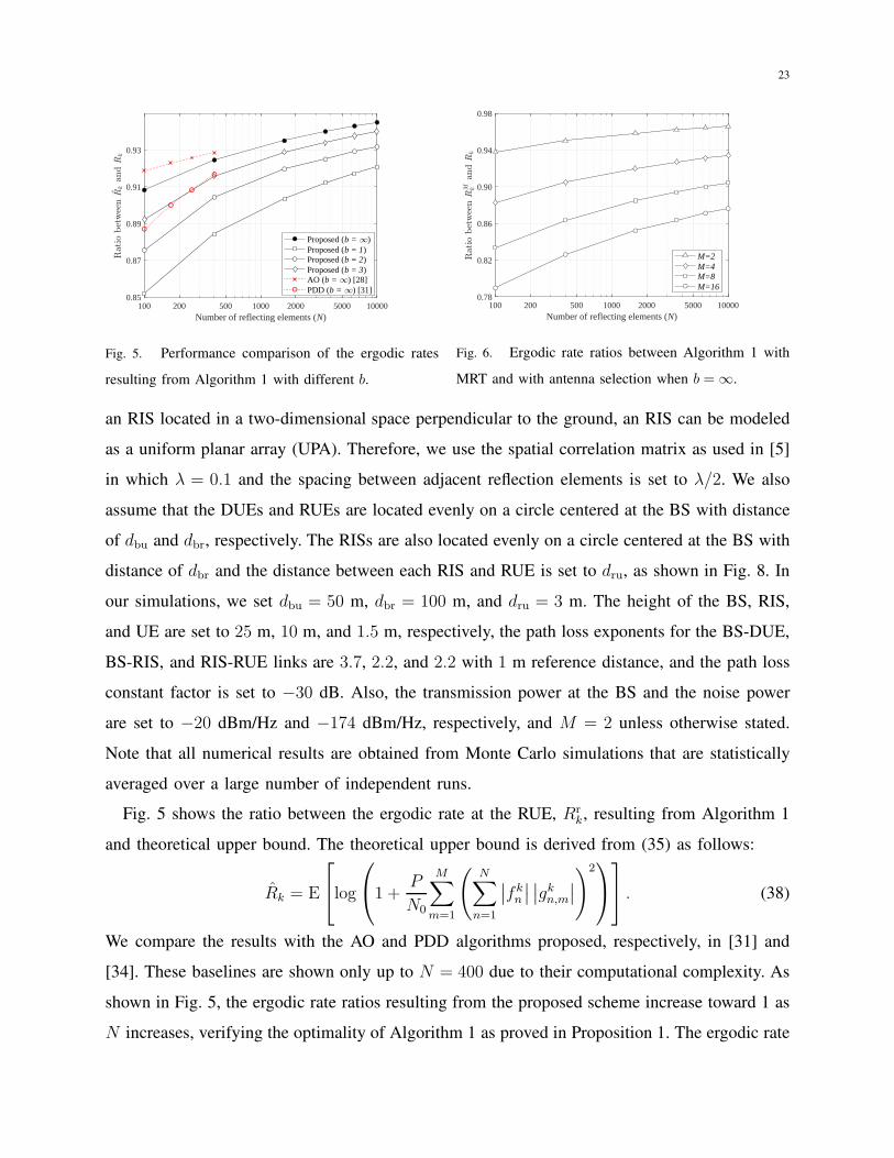
Fig. 5 shows the ratio between the ergodic rate at the RUE, Rrk, resulting from Algorithm 1
and theoretical upper bound. The theoretical upper bound is derived from (35) as follows:
Rk = E
log
1 +P
N0
M∑
m=1
(
N∑
n=1
∣
∣fkn
∣
∣
∣
∣gkn,m∣
∣
)2
. (38)
We compare the results with the AO and PDD algorithms proposed, respectively, in [31] and
[34]. These baselines are shown only up to N = 400 due to their computational complexity. As
shown in Fig. 5, the ergodic rate ratios resulting from the proposed scheme increase toward 1 as
N increases, verifying the optimality of Algorithm 1 as proved in Proposition 1. The ergodic rate

24
-30 -20 -10 0 10 20SNR (dB)
10-5
10-4
10-3
10-2
10-1
SER
SimulationEstimation
N increases(N=16, 32, 64, 128, 256, 512)
Fig. 7. Comparison of the average SERs resulting from
the proposed modulation with different N values.
Fig. 8. An example of our simulation environment (top
view) when K = 8.
ratio resulting from the proposed scheme with b = ∞ is higher than the one resulting from the
PDD algorithm, since the PDD algorithm does not consider the reflection power loss. Although
the AO algorithm can achieve the upper bound performance, asymptotically, it requires very
high complexity. In both the AO and PDD algorithms, a complexity in the order of O (N2)
is required for each iteration [31], [34]. However, the proposed Algorithm 1 requires O (N)
resulting in a much simpler operation at the BS especially for a large N . Moreover, the AO
algorithm uses MRT which requires multiple RF chains resulting in higher cost and hardware
complexity compared to the proposed algorithm.
Fig. 6 shows the ratios between the ergodic rates resulting from Algorithm 1 with MRT, RMk ,
and with antenna selection for different M values. As shown in Fig. 6, the ergodic rate ratios
decrease as M increases, however, all results increase toward 1 as N increases, verifying that
the transmit antenna selection asymptotically achieves the performance of the MRT.
In Fig. 7, Theorem 1 is verified in the following scenario. The BS transmits BPSK signals to
the sDUE via a wireless channel, hk, and also sends the RIS control signals related to the data
symbols for the uRIS via a dedicated RIS control link. Data symbols for the uRIS are modulated
based on the proposed modulation technique assuming the BPSK signaling (i.e., M0 = 2) and
all channels are generated by independent Rayleigh fading to verify Theorem 1. As shown in
Fig. 7, the asymptotic SERs derived from Theorem 1 are close to the results of our simulations.
Moreover, the SERs linearly decrease as N increases given that the SNR difference is always
equal to 3 dB when N is doubled. For instance, when the target SER is 2·10−2, the corresponding

25
0 400 800 1200 1600Time slot
2.05
2.1
2.15
2.2
2.25
Ave
rage
sum
-rat
e (b
ps)
108
N=100N=144N=225
Fig. 9. Convergence of the average sum-rate resulting from Algorithm 2.
SNRs are 5, 2, −1, −4, −7, −10 dB for N = 16, 32, 64, 128, 256, 512, respectively. This result
shows that the SER can be reduced by increasing N and eventually it converges to zero as
N → ∞.
In Figs. 9–11, Algorithm 2 is verified in the following scenario. The average transmission
power at the BS and the noise power are set to −20 dBm/Hz and −174 dBm/Hz, respectively,
and 10 UEs (5 DUE and 5 RUE) are located around the BS with b = 1 unless otherwise
stated. We consider an OFDMA system where the system bandwidth is 10 MHz and the whole
bandwidth is equally divided into 25 RBs (i.e., F = 25), and the minimum rate requirement is
set to 20 Mbps per UE.
Fig. 9 shows the convergence of the average sum-rate resulting from Algorithm 2. This
convergence shows that Algorithm 2 always satisfies the constraints of the transmission power
and the rate requirements in (27) regardless of N , verifying the convergence of Algorithm 2.
Also, the convergence is satisfied within seconds after initial access (e.g., 1 ms ×1000 TTIs =
1.0 s) regardless of N , showing that the optimal sum-rate can be achieved within a few seconds.
Figs. 10 and 11 compare the average data rates resulting from Algorithm 2 with and without
the minimum rate requirements. As proved in Proposition 1, the received SNRs at the RUEs
increase with O (N2) while those at the DUEs approximately keep constant as N increases. For
a large N without considering the rate requirements, Algorithm 2 selects more RUEs than DUEs
for better sum-rate resulting in unfairness of individual rates, as shown in Fig. 10. However, in
this case, we can achieve better performance in terms of the average sum-rate compared to the
case in which the UEs have the requirements on the minimum rates, as shown in Fig. 11. On
the other hand, when we consider the minimum rate requirements, all individual rates satisfy

26
DUE 1 DUE 2 DUE 3 DUE 4 DUE 5 RUE 1 RUE 2 RUE 3 RUE 4 RUE 50
0.5
1
1.5
2
2.5
3
Ave
rage
rat
e (b
ps)
107
Rate requirement (20 Mbps)With rate requirementWithout rate requirement
Fig. 10. Average individual rates at each UE with and
without R when N = 100.
100 300 500 700 900Number of reflecting elements (N)
2
2.5
3
3.5
4
4.5
5
Ave
rage
sum
-rat
e (b
ps)
108
With rate requirementWithout rate requirement
K=10
K=20
K=40
Fig. 11. Performance comparison of the average sum-
rates for cases with and without R.
those requirements while the average sum-rate decreases, as shown in Figs. 10 and 11. Hence,
Algorithm 2 can control the tradeoff between fairness and maximum performance. Since the
BS serves a single UE at each RB, the user selection gain resulting from R = maxk∈R
Rk will be
limited at high SNR region. However, since the additional sum-rate is calculated by the sum of
|R| additional rates from all uRUEs, the additional sum-rate linearly increases as K increases.
This additional sum-rate gradually increases its effects on the average sum-rate as N and K
increase as shown in Fig. 11, showing that our algorithm can support massive connectivity.
V. CONCLUSIONS
In this paper, we have asymptotically analyzed the optimality of the achievable rate using
practical RISs in presence of limitations such as practical reflection coefficients and limited RIS
control link capacity. In particular, we have designed a passive beamformer that can achieve
the asymptotic optimal SNR under discrete reflection phases with a practical reflection power
loss, and shown that it achieves a SNR optimality even with one bit RIS control. We have also
proposed a modulation scheme that can be used in a downlink RIS system resulting in higher
achievable sum-rate than a conventional network without RIS. Moreover, we have derived the
approximated SER of the proposed modulation scheme, showing that it achieves an asymptotic
SNR of a conventional massive array systems such as a massive MIMO or MIMO relay system.
Furthermore, we have proposed the resource allocation algorithm under consideration of the
aforementioned passive beamforming and the modulation schemes that achieves the asymptotic
optimal sum-rate. We have shown that the proposed algorithms can analytically achieve the
performance of an ideal RIS. Simulation results have shown that the results of our algorithms
27
converge to the asymptotic upper bound as N → ∞. In particular, we have observed that the
approximated SER is in close agreement with the result from our simulations and the proposed
resource allocation algorithm asymptotically achieves the optimal performance satisfying the
minimum rate requirements at each UE. Moreover, our results have shown that the proposed
resource algorithm can control the tradeoff between fairness of individual performance and
maximum system performance. We finally have shown that the performance of our algorithm
increases as the number of UEs increases, resulting from the additional rate achieved at the
uRUEs. Therefore, we expect that our algorithm will be invaluable solution for future wireless
networks supporting massive connectivity. Our future work will include extending our results
to additional practical scenarios such as a multi-user MIMO OFDM system that has an RIS
environment with a finite number of reflecting elements and multi-hop reflections.
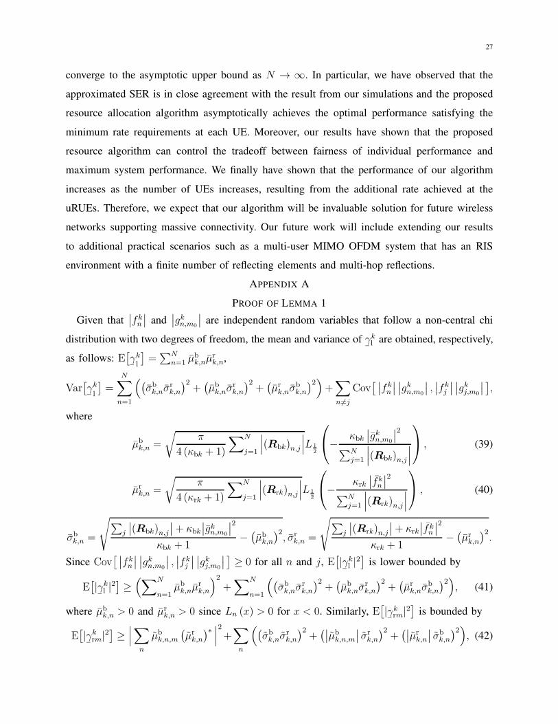
APPENDIX A
PROOF OF LEMMA 1
Given that∣
∣fkn
∣
∣ and∣
∣gkn,m0
∣
∣ are independent random variables that follow a non-central chi
distribution with two degrees of freedom, the mean and variance of¯γkl are obtained, respectively,
as follows: E[
¯γkl
]
=∑N
n=1 µbk,nµ
rk,n,
Var[
¯γk
l
]
=N∑
n=1
(
(
σbk,nσ
rk,n
)2+(
µbk,nσ
rk,n
)2+(
µrk,nσ
bk,n
)2)
+∑
n 6=j
Cov[ ∣
∣fkn
∣
∣
∣
∣gkn,m0
∣
∣ ,∣
∣fkj
∣
∣
∣
∣gkj,m0
∣
∣
]
,
where
µbk,n =
√
π
4 (κbk + 1)
∑N
j=1
∣
∣
∣(Rbk)n,j
∣
∣
∣L 1
2
− κbk
∣
∣gkn,m0
∣
∣
2
∑Nj=1
∣
∣
∣(Rbk)n,j
∣
∣
∣
, (39)
µrk,n =
√
π
4 (κrk + 1)
∑N
j=1
∣
∣
∣(Rrk)n,j
∣
∣
∣L 1
2
− κrk
∣
∣fkn
∣
∣
2
∑Nj=1
∣
∣
∣(Rrk)n,j
∣
∣
∣
, (40)
σbk,n =
√
∑
j
∣
∣(Rbk)n,j∣
∣+ κbk
∣
∣gkn,m0
∣
∣
2
κbk + 1−(
µbk,n
)2, σr
k,n =
√
∑
j
∣
∣(Rrk)n,j∣
∣+ κrk
∣
∣fkn
∣
∣
2
κrk + 1−(
µrk,n
)2.
Since Cov[ ∣
∣fkn
∣
∣
∣
∣gkn,m0
∣
∣ ,∣
∣fkj
∣
∣
∣
∣gkj,m0
∣
∣
]
≥ 0 for all n and j, E[
|¯γkl |2]
is lower bounded by
E[
|¯γkl |2]
≥(
∑N
n=1µbk,nµ
rk,n
)2
+∑N
n=1
(
(
σbk,nσ
rk,n
)2+(
µbk,nσ
rk,n
)2+(
µrk,nσ
bk,n
)2)
, (41)
where µbk,n > 0 and µr
k,n > 0 since Ln (x) > 0 for x < 0. Similarly, E[
|¯γkrm|2
]
is bounded by
E[
|¯γkrm|2
]
≥∣
∣
∣
∑
n
µbk,n,m
(
µrk,n
)∗∣
∣
∣
2
+∑
n
(
(
σbk,nσ
rk,n
)2+(∣
∣µbk,n,m
∣
∣ σrk,n
)2+(∣
∣µrk,n
∣
∣ σbk,n
)2)
, (42)

28
where
µbk,n,m=
√
κbk
κbk + 1gkn,m, µ
rk,n=
√
κrk
κrk + 1fkn , σ
bk,n=
√
∑Nj=1
∣
∣(Rbk)n,j∣
∣
κbk + 1, σr
k,n=
√
∑Nj=1
∣
∣(Rrk)n,j∣
∣
κrk + 1.
Given the definition of¯γk
from (14), we have
E[
¯γk
]
≥ PErk |Γ|2min
N0
(
E[
|¯γkl |2]
+∑M
m6=m0
E[
|¯γkrm|2
]
)
≥ PErk |Γ|2min
N0
{
(
∑N
n=1µbk,nµ
rk,n
)2
+∑N
n=1
(
(
σbk,nσ
rk,n
)2+(
µbk,nσ
rk,n
)2+(
µrk,nσ
bk,n
)2)
+
M∑
m6=m0
∣
∣
∣
∣
∣
N∑
n=1
µbk,n,mµ
r∗k,n
∣
∣
∣
∣
∣
2
+
N∑
n=1
(
(
σbk,nσ
rk,n
)2+(∣
∣µbk,n,m
∣
∣ σrk,n
)2+(∣
∣µrk,n
∣
∣ σbk,n
)2)
(43)
In order to verify the scaling law of (43), we first determine the scaling law of(∑
n µbk,nµ
rk,n
)2in
(43) according to N . Since we consider an RIS located in a two-dimensional space perpendicular
to the ground, it can be modeled as a UPA [5], [44]. Hence, we have∑N
j=1 |(Rbk)n,j| =∑N
j=1 |(Rbk)n,j| = 1. From the scaling law for N ,(∑
n µbk,nµ
rk,n
)2in (43) is then calculated
by the squared sum of positive N elements and increases with O (N2). On the other hand,∑
n
(
(
σbk,nσ
rk,n
)2+(
µbk,nσ
rk,n
)2+(
µrk,nσ
bk,n
)2)
in (43) is calculated by the sum of positive N
elements resulting in O (N) and becomes negligible compared to(∑
n µbk,nµ
rk,n
)2as N increases.
Similarly, the other term in (43) follows O (N) and also become negligible as N increases.
Therefore, (43) eventually converges toPEr
k|Γ|2min
N0
(∑
n µbk,nµ
rk,n
)2, which completes the proof.
APPENDIX B
PROOF OF THEOREM 1
Given that the maximum instantaneous SNR at sDUE k can be achieved by using the MRT
such as wk = hk/ ‖hk‖, the instantaneous SNR at uRUE i can be derived by using (22) as
γuRi =
PA(ωi)2NsE
dk
∣
∣fHi Gihk
∣
∣
2
N0‖hk‖2. (44)
Since the uRIS transmits the same symbols during the data transmission period, the uRUE
achieves the diversity gain proportional to Ns resulting in Ns-fold of the desired signal power
as shown in (44). In order to verify the scaling law of the average SNR at uRUE i, we first
determine the scaling law of E[
|fHi Giwk|2
]
for N . From (42), E[
|fHi Giwk|2
]
is bounded as
E[
|fHi Giwk|2
]
≥∣
∣
∣
∑
mE[
wkm
]
¯µi,m
∣
∣
∣
2
+∑
m
(
Var[
wkm
]
¯σ2i,m +
∣
∣
¯µi,m
∣
∣
2Var[
wkm
]
+∣
∣E[
wkm
]∣
∣
2
¯σ2i,m
)
,

29
where¯µi,m=
∑Nn=1 µ
bi,n,m
(
µri,n
)∗and
¯σ2i,m=
∑Nn=1
(
(
σbi,nσ
ri,n
)2+(∣
∣µbi,n,m
∣
∣ σri,n
)2+(∣
∣µri,n
∣
∣ σbi,n
)2)
.
From the scaling law for N , the lower bound increases with O (N) as N increases. Therefore,
the uRUE can achieve average SNR in order of O (N).
As a special case, we can analyze the average SNR at uRUE i for i.i.d. Rayleigh fading
channels by assuming that κbk = κrk = κdk = 0 and Rbk = Rrk = IN . In order to
analyze the impact on (44) of the number of BS antennas, we consider two exteme cases:
M = 1 and M → ∞. We first analyze (44) when M = 1. Then, (44) is obtained by
γuRi = PA(ωi)
2NsEdk
∣
∣
∣
∑Nn=1 f
i∗n gin
∣
∣
∣
2
/N0. By using the CLT,∑N
n=1 fi∗n gin converges to a complex
Gaussian distributed random variable with zero mean and variance of N . Then, we have
1
NγuRi
d−−−→N→∞
PA(ωi)2NsE
dk
2N0χ22, (45)
where “d−−−−→
M→∞” denotes the convergence in distribution and χ2
k denotes the chi-squared distri-
bution with k degress of freedom. We consider a random variable Y1 as γuRi when M = 1. Then,
the mean and the probability density function (PDF) of Y1 can be obtained, respectively, as
E [Y1] =PA(ωi)
2NNsEdk
N0
, fY1(y) =
N0
PA(ωi)2NNsEd
k
e−
N0y
PA(ωi)2NNsE
dk . (46)
Next, we analyze (44) as M → ∞. Then, (44) can be obtained by:
γuRi = lim
M→∞
PA(ωi)2NsE
dk
∣
∣
∣
∑Mm=1 h
km
∑Nn=1 f
i∗n gin,m
∣
∣
∣
2
N0
∑Mm=1 |hk
m|2 , (47)
where hk =[
hk1, · · · , hk
M
]T. On the basis of the CLT for a large M ,
∑Mm=1 h
km
∑Nn=1 f
i∗n gin,m in
(47) converges to a complex Gaussian distributed random variable with zero mean and variance
of NM . Hence, we have 1M
∣
∣
∣
∑Mm=1 h
km
∑Nn=1 f
i∗n gin,m
∣
∣
∣
2 d−−−−→M→∞
N2χ22. Also, the denominator in
(47) follows the chi-squared distribution: N0
∑Mm=1
∣
∣hkm
∣
∣
2 ∼ N0
2χ22M . Note that the distribution
of the ratio of two chi-squared distributed random variables is the beta prime distribution [45].
Considering a random variable YM as γuRi with a large M , the mean and the PDF of YM can
be obtained based on the beta prime distribution, respectively:
E [YM ] =PA(ωi)
2NMNsEdk
N0 (M − 1), (48)
fYM(y) =
N0
PA(ωi)2NNsEd
k
(
1 +N0y
PA(ωi)2NMNsEd
k
)−M−1
. (49)

30
As M → ∞, (48) and (49) are obtained, respectively, as follows:
E [Y∞] = limM→∞
E [YM ] = PA(ωi)2NNsE
dk/N0, (50)
fY∞(y) = lim
M→∞fYM
(y) =(c)
N0
PA(ωi)2NNsE
dk
e−
N0y
PA(ωi)2NNsE
dk , (51)
where (c) is obtained from the exponential function definition ex = limn→∞
(1 + x/n)n. Hence,
we can obtain the following equalities: E [Y1] = E [Y∞] and fY1(y) = fY∞
(y) . Since the
transmit precoder at the BS is designed to match hk independent with fHi Gi, the moments of
instantaneous SNR at the uRUE will be a monotonic function with respect to M . Therefore,
γuRi can be approximated as the chi-squared distributed random variable given in (45) regardless
of M . By using the characteristic of a chi-squared distribution, γuRi has the following moment
generating function (MGF) [46]: MγuRi
(µp, t) = 1
1−NNsEsA(µp)2t
N0
. Based on this MGF, we can
obtain the average SER of the proposed M0-PSK signal at the uRUE as follows [47]:
Pe =1
2Mo
2Mo∑
p=1
ˆ π−∆µ
2
0
MγuRi
(
µp,−sin2 (∆µ/2)
sin2θ
)
dθ. (52)
APPENDIX C
PROOF OF PROPOSITION 2
The integer solution qt,fk always has a value of 0 or 1 for the entire range of P t,f . If we
can calculate the optimal P t,f that maximizes Rt,fk for each qt,fk = 1, k ∈ K and f ∈ F (i.e.,
qt,fi = 0, ∀i 6= k ∈ K and f ∈ F ), we can jointly find the optimal P t,f and qt,fk by comparing
those maximum Rt,fk values. Since γt,f
dk , γt,fai , and γt,f
rk in (33) are strictly concave functions with
respect to P t,f , Rt,fk −µP t,f is also a concave function with respect to P t,f . For k ∈ R, we can
readily find the maximizer P t,fk by letting the first derivative be zero under consideration of the
power constraint in (31a):
P t,fk =
1 + λk
µ− N0∣
∣
∣
(
ft,fk
)H
Φt,f
k gt,fk
∣
∣
∣
2
Pmax
0
, k ∈ R, f ∈ F , (53)
where [x]ba = a if x < a, [x]ba = b if x > b, and otherwise, [x]ba = x. For k ∈ D, we can also
obtain the globally optimal P t,fk using a simple gradient method under the constraint in (31a).
From those results of P t,fk , ∀k ∈ K and ∀f ∈ F , we can find the optimal qt,fk as in (34) and the
corresponding P t,fk is the optimal transmission power, which completes the proof.
31
REFERENCES
[1] Q. Wu and R. Zhang, “Beamforming optimization for wireless network aided by intelligent reflecting surface with discrete
phase shifts,” IEEE Transactions on Communications, vol. 68, no. 3, pp. 1838–1851, 2020.
[2] W. Saad, M. Bennis, and M. Chen, “A vision of 6G wireless systems: Applications, trends, technologies, and open research
problems,” IEEE Network, to appear, 2020.
[3] M. Mozaffari, A. T. Z. Kasgari, W. Saad, M. Bennis, and M. Debbah, “Beyond 5G with UAVs: Foundations of a 3D
wireless cellular network,” IEEE Trans. Commun., vol. 18, no. 1, pp. 357–372, Jan. 2019.
[4] M. Jung, W. Saad, Y. Jang, G. Kong, and S. Choi, “Reliability analysis of large intelligent surfaces (LISs): Rate distribution
and outage probability,” IEEE Wireless Communications Letters, vol. 8, no. 6, pp. 1662–1666, Dec. 2019.
[5] M. Jung, W. Saad, Y. Jang, G. Kong, and S. Choi, “Performance analysis of large intelligent surfaces (LISs): Asymptotic
data rate and channel hardening effects,” IEEE Trans. Wireless Commun., vol. 19, no. 3, pp. 2052–2065, Mar. 2020.
[6] C. Chaccour, M. N. Soorki, W. Saad, M. Bennis, and P. Popovski, “Risk-based optimization of virtual reality over terahertz
reconfigurable intelligent surfaces,” in IEEE ICC, Dublin, Ireland, Jun. 2020.
[7] T. J. Cui, S. Liu, and L. Zhang, “Information metamaterials and metasurfaces,” Journal of Materials Chemistry C, vol. 5,
pp. 3644–3668, 2017.
[8] E. Basar, M. D. Renzo, J. de Rosny, M. Debbah, M. S. Alouini, and R. Zhang, “Wireless communications through
reconfigurable intelligent surfaces,” IEEE Access, vol. 7, pp. 116 753–117 773, Sep. 2019.
[9] W. Tang, J. Y. Dai, M. Chen, X. Li, Q. Cheng, S. Jin, K. Wong, and T. J. Cui, “Programmable metasurface-based RF
chain-free 8PSK wireless transmitter,” Electronics Letters, vol. 55, no. 7, pp. 417–420, 2019.
[10] W. Tang, X. Li, J. Y. Dai, S. Jin, Y. Zeng, Q. Cheng, and T. J. Cui, “Wireless communications with programmable
metasurface: Transceiver design and experimental results,” available online: arxiv.org/abs/1811.08119, Nov. 2018.
[11] Q. Wu and R. Zhang, “Intelligent reflecting surface enhanced wireless network via joint active and passive beamforming,”
IEEE Transactions on Wireless Communications, vol. 18, no. 11, pp. 5394–5409, Nov. 2019.
[12] Y. Han, W. Tang, S. Jin, C. Wen, and X. Ma, “Large intelligent surface-assisted wireless communication exploiting statistical
CSI,” IEEE Transactions on Vehicular Technology, vol. 68, no. 8, pp. 8238–8242, Aug. 2019.
[13] C. Huang, G. Alexandropoulos, A. Zaponne, M. Debbah, and C. Yuen, “Energy efficient multi-user MISO communication
using low resolution large intelligent surfaces,” in IEEE GLOBECOM, Abu Dhabi, UAE, Dec. 2018.
[14] M. Jung, W. Saad, M. Debbah, and C. S. Hong, “Asymptotic optimality of reconfigurable intelligent surfaces: Passive
beamforming and achievable rate,” in IEEE ICC, Dublin, Ireland, Jun. 2020.
[15] D. F. Sievenpiper, J. H. Schaffner, H. J. Song, R. Y. Loo, and G. Tangonan, “Two-dimensional beam steering using an
electrically tunable impedance surface,” IEEE Trans. Antennas Propag., vol. 51, no. 10, pp. 2713–2722, Oct. 2003.
[16] B. O. Zhu, J. Zhao, and Y. Feng, “Active impedance metasurface with full 360 reflection phase tuning,” Scientific Reports,
vol. 3, pp. 3059–3064, Oct. 2013.
[17] S. Hu, F. Rusek, and O. Edfors, “Beyond massive MIMO: The potential of data transmission with large intelligent surfaces,”
IEEE Trans. Signal Process., vol. 66, no. 10, pp. 2746–2758, May 2018.
[18] Y. Huang, X. Guan, H. Chen, Y. Liang, S. Yuan, and T. Ohtsuki, “Risk assessment of private information inference for
motion sensor embedded IoT devices,” IEEE Trans. Emerg. Topics Comput. Intell., vol. 4, no. 3, pp. 265–275, Jun. 2020.
[19] Z. Zhang, H. Chen, M. Hua, C. Li, Y. Huang, and L. Yang, “Double coded caching in ultra dense networks: Caching and
multicast scheduling via deep reinforcement learning,” IEEE Trans. Commun., vol. 68, no. 2, pp. 1071–1086, 2020.

32
[20] J. Jhao, “A survey of intelligent reflecting surfaces (IRSs): Towards 6G wireless communication networks,” available
online: arxiv.org/abs/1907.04789, Jul. 2019.
[21] Q. Wu and R. Zhang, “Towards smart and reconfigurable environment: Intelligent reflecting surface aided wireless network,”
IEEE Commun. Mag., vol. 58, no. 1, pp. 106–112, 2020.
[22] C. Pan, H. Ren, K. Wang, M. Elkashlan, A. Nallanathan, J. Wang, and L. Hanzo, “Intelligent reflecting surface enhanced
MIMO broadcasting for simultaneous wireless information and power transfer,” available online: arxiv.org/abs/1908.04863,
Feb. 2020.
[23] Q. Wu and R. Zhang, “Joint active and passive beamforming optimization for intelligent reflecting surface assisted SWIPT
under QoS constraints,” IEEE Journal of Selected Areas in Communications, to appear, 2020.
[24] M. Cui, G. Zhang, and R. Zhang, “Secure wireless communication via intelligent reflecting surface,” IEEE Wireless
Communications Letters, vol. 8, no. 5, pp. 1410–1414, Oct. 2019.
[25] N. Rajatheva et al., “White paper on broadband connectivity in 6G,” available online: arxiv.org/abs/2004.14247, Apr.
2020.
[26] Samsung Research, “The next hyper-connected expereience for all,” 6G White Paper, available online:
https://research.samsung.com, Jul. 2020.
[27] N. Rajatheva et al., “Scoring the terabit/s goal: Broadband connectivity in 6G,” available online: arxiv.org/abs/2008.07220,
Aug. 2020.
[28] 3rd Generation Partnership Project, “Technical Specification Group Radio Access Network; User Equipment (UE)
conformance specification; Radio transmission and reception; Part 1: Conformance testing,” TS 36.521-1, V14.3.0, 2017.
[29] M. Chiani, A. Conti, M. Mazzotti, E. Paolini, and A. Zanella, “Outage capacity for MIMO-OFDM systems in block fading
channels,” in Asilomar Conference on Signals, Systems and Computers (ASILOMAR), Nov. 2011.
[30] 3rd Generation Partnership Project, “Technical Specification Group Radio Access Network; Physical layer procedures for
data,” TS 38.214, V15.2.0, Jul. 2018.
[31] S. Abeywickrama, R. Zhang, and C. Yuen, “Intelligent reflecting surface: Practical phase shift model and beamforming
optimization,” available online: arxiv.org/abs/2002.10112, Feb. 2020.
[32] H. Q. Ngo, E. G. Larsson, and T. L. Marzetta, “Energy and spectral efficiency of very large multiuser MIMO systems,”
IEEE Transactions on Communications, vol. 61, no. 4, pp. 1436–1449, Apr. 2013.
[33] D. Tse and P. Viswanath, Fundamentals of Wireless Communication. Cambridge Univ. Press, 2005.
[34] M.-M. Zhao, Q. Wu, M.-J. Zhao, and R. Zhang, “Intelligent reflecting surface enhanced wireless network: Two-timescale
beamforming optimization,” available online: arxiv.org/abs/1912.01818, Sep. 2020.
[35] S. Sanayei et al., “Antenna selection in MIMO systems,” IEEE Commun. Mag., vol. 42, no. 10, pp. 68–73, Oct. 2004.
[36] V. C. Liu, A. N. Parks, V. Talla, S. Gollakota, D. Wetherall, and J. S. R. Smith, “Ambient backscatter: wireless
communication out of thin air,” in ACM Special Interest Group on Data Communication (SIGCOMM), 2013.
[37] 3rd Generation Partnership Project, “Technical Specification Group Radio Access Network; Physical layer procedures,”
TS 36.213, V14.6.0, Apr. 2018.
[38] ——, “Technical Specification Group Radio Access Network; Multiplexing and channel coding,” TS 36.212, V14.2.0,
2017.
[39] ——, “Technical Specification Group Radio Access Network; Physical channels and modulation,” TR 36.211, V15.0.0,
Dec. 2017.

33
[40] J.-W. Lee, R. R. Mazumdar, and N. B. Shroff, “Opportunistic power scheduling for dynamic multi-server wireless systems,”
IEEE Transactions on Wireless Communications, vol. 5, no. 6, pp. 1506–1515, Jun. 2006.
[41] Y. Ermoliev, “Stochastic quasigradient methods and their application to system optimization,” Stochastics, vol. 9, 1983.
[42] P. Kall and S. W. Wallace, Stochastic Programming. Wiley, 1994.
[43] D. P. Bertsekas, Nonlinear Programming. Athena Scientific, 1999.
[44] J. Song, J. Choi, and D. J. Love, “Common codebook millimeter wave beam design: Designing beams for both sounding
and communication with uniform planar arrays,” IEEE Trans. Commun., vol. 65, no. 4, pp. 1859–1872, Apr. 2017.
[45] N. L. Johnson, S. Kotz, and N. Balakrishnan, Continuous Univariate Distributions. Wiley, 1995.
[46] J. G. Proakis, Digital Communications. New York: MCGraw-Hilll, 2008.
[47] M. Simon and M. S. Alaouni, Digital Communications over Fading Channels. New Jersey: John Wiley & Sons, 2005.


![Reconfigurable Intelligent Surfaces: Principles and …intelligence [1], [2]. Therefore, new transmission technologies are needed in order to support these new applications and services](https://img.pdfslide.us/doc/110x75/60cbf8332e1e225e0f6741aa/reconigurable-intelligent-surfaces-principles-and-intelligence-1-2-therefore.jpg)