Embed Size (px)
Citation preview
arX
iv:1
908.
0744
5v1
[cs
.IT
] 1
7 A
ug 2
019
1
On the Differential-Linear Connectivity Table
of Vectorial Boolean Functions
Anne Canteaut, Lukas Kölsch, Chao Li, Chunlei Li,
Kangquan Li, Longjiang Qu and Friedrich Wiemer
Abstract
Vectorial Boolean functions are crucial building-blocks in symmetric ciphers. Different known attacks
on block ciphers have resulted in diverse cryptographic criteria for vectorial Boolean functions, such as
differential uniformity and nonlinearity. Very recently, Bar-On et al. introduced at Eurocrypt’19 a new tool,
called the differential-linear connectivity table (DLCT), which allows for taking into account the dependency
between the two subciphers E0 and E1 involved in differential-linear attacks. This new notion leads to
significant improvements of differential-linear attacks on several ciphers. This paper presents a theoretical
characterization of the DLCT of vectorial Boolean functions and also investigates this new criterion for
some families of functions with specific forms.
More precisely, we firstly reveal the connection between the DLCT and the autocorrelation of vectorial
Boolean functions, we characterize properties of the DLCT by means of the Walsh transform of the function
and of its differential distribution table, and we present generic bounds on the highest magnitude occurring
in the DLCT of vectorial Boolean functions, which coincides (up to a factor 2) with the well-established
notion of absolute indicator. Next, we investigate the invariance property of the DLCT of vectorial Boolean
functions under the affine, extended-affine, and Carlet-Charpin-Zinoviev (CCZ) equivalence and exhaust
the DLCT spectra of optimal 4-bit S-boxes under affine equivalence. Furthermore, we study the DLCT of
APN, plateaued and AB functions and establish its connection with other cryptographic criteria. Finally,
we investigate the DLCT and the absolute indicator of some specific polynomials with optimal or low
differential uniformity, including monomials, cubic functions, quadratic functions and inverses of quadratic
permutations.
1. INTRODUCTION
Let n,m be two arbitrary positive integers. We denote by F2n the finite field with 2n elements and by
Fn2 the n-dimensional vector space over F2. Vectorial Boolean functions from F
n2 to F
m2 , also called (n,m)-
functions, play a crucial role in block ciphers. Many attacks have been proposed against block ciphers, and
Anne Canteaut is with Inria, Paris, France. Lukas Kölsch is with University of Rostock, Germany. Chunlei Li is with the
Department of Informatics, University of Bergen, Bergen N-5020, Norway. Kangquan Li, Longjiang Qu and Chao Li are with the
College of Liberal Arts and Sciences, National University of Defense Technology, Changsha, 410073, China. Longjiang Qu is also
with the State Key Laboratory of Cryptology, Beijing, 100878, China. Friedrich Wiemer is with the Horst Görtz Institute for IT
Security, Ruhr University Bochum, Germany. Emails: [email protected], [email protected], [email protected],
[email protected], [email protected], [email protected], [email protected]
2
have led to diverse criteria, such as low differential uniformity, high nonlinearity, high algebraic degree, etc,
that the implemented cryptographic functions must satisfy. In Eurocrypt’18, Cid et al. [18] introduced a
new concept on S-boxes: the boomerang connectivity table (BCT) that similarly analyzes the dependency
between the upper part and lower part of a block cipher in a boomerang attack. The work of [18] quickly
attracted attention in the study of BCT property of cryptographic functions [6], [29], [34], [39] and stimulated
research progress in other cryptanalysis methods. Very recently, in Eurocrypt’19, Bar-On et al. [1] introduced
a new tool called the differential-linear connectivity table (DLCT) that analyzes the dependency between
the two subciphers in differential-linear attacks, thereby improving the efficiency of the attacks introduced
in [26]. The authors of [1] also presented the relation between the DLCT and the differential distribution
table (DDT) of S-boxes.
This paper aims to provide a theoretical characterization of the main properties of the DLCT, explicitly
of the set formed by all its entries and of the highest magnitude in this set, for generic vectorial Boolean
functions. To this end, we firstly show that the DLCT coincides (up to a factor 2) with the autocorrelation
of vectorial Boolean functions, which is extended from Boolean functions. Based on the study of the
autocorrelation of vectorial Boolean functions, we give some characterizations of the DLCT by means of the
Walsh transform and the DDT, and provide a lower bound on the absolute indicator (i.e., equivalently, on the
highest absolute value in the DLCT excluding the first row and first column) of any (n,m)-function; then we
exhibit an interesting divisibility property of the autocorrelation of (n,m)-functions F , which implies that the
entries of DLCT of any (n, n)-permutations are divisible by 4. Next, we investigate the invariance property
of the autocorrelation (and the DLCT) of vectorial Boolean functions under affine, extended-affine (EA) and
Carlet-Charpin-Zinoviev (CCZ) equivalence, and show that the autocorrelation spectrum is affine-invariant
and its maximum magnitude is EA-invariant but not CCZ-invariant. Based on the classification of optimal
4-bit S-boxes by Leander and Poschmann [27], we explicitly calculate their autocorrelation spectra (see
Table II). Moreover, for certain functions like APN, plateaued and AB functions, we present the relation of
their autocorrelation (and DLCT) with other cryptographic criteria. We show that the autocorrelation of APN
and AB/plateaued functions can be converted to the Walsh transform of two classes of balanced Boolean
functions. Finally, we investigate the autocorrelation spectra of some special polynomials with optimal or low
differential uniformity, including monomials, cubic functions, quadratic functions and inverses of quadratic
permutations.
The rest of this paper is organized as follows. Section 2 recalls basic definitions, particularly the new notion
of DLCT, the generalized notion of autocorrelation, and the connection between them. Most notably, we show
that the highest magnitude in the DLCT coincides (up to a factor 2) with the absolute indicator of the function.
Section 3 is devoted to the characterization of the autocorrelation: we firstly characterize the autocorrelation
by means of the Walsh transform and of the DDT of the function. We then exhibit generic lower bounds
on the absolute indicator of any vectorial Boolean function and study the divisibility of the autocorrelation
coefficients. Besides, we study the invariance of the absolute indicator and of the autocorrelation spectrum
under the affine, EA and CCZ equivalences. We also present all possible autocorrelation spectra of optimal
3
4-bit S-boxes. At the end of this section, we study some properties of the autocorrelation of APN, plateaued
and AB functions. In Section 4, we consider the autocorrelation of some special polynomials. Finally, Section
5 draws some conclusions of our work.
2. PRELIMINARIES
In this section, we firstly recall some basics on (vectorial) Boolean functions and known results that are
useful for our subsequent discussions. Since the vector space Fn2 can be deemed as the finite field F2n for
a fixed choice of basis, we will use the notation Fn2 and F2n interchangeably when there is no ambiguity.
We will also use the inner product a · b and Tr2n(ab) in the context of vector spaces and finite fields
interchangeably. For any set E, we denote the nonzero elements of E by E∗ (or E \{0}) and the cardinality
of E by #E.
A. Walsh transform, Bent functions, AB functions and Plateaued functions
An n-variable Boolean function is a mapping from Fn2 to F2. For any n-variable Boolean function f , its
Walsh transform of f is defined as
Wf (ω) =∑
x∈Fn2
(−1)f(x)+ω·x,
where “ · ” is an inner product on Fn2 . The Walsh transform of f can be seen as the discrete Fourier
transform of the function (−1)f(x) and yields the well-known Parseval’s relation [14] :
∑
ω∈Fn2
W 2f (ω) = 22n.
The linearity of f is defined by
L(f) = maxω∈Fn
2
|Wf (ω)|
and nonlinearity of f is defined by
NL(f) = 2n−1 −1
2L(f),
where |r| denotes the absolute value of any real value r. According to the Parseval’s relation, it is easily
seen that the nonlinearity of an n-variable Boolean function is upper bounded by 2n−1 − 2n/2−1. Boolean
functions achieving the maximum nonlinearity are called bent functions and exist only for even n; their
Walsh transforms take only two values ±2n/2 [37].
For an (n,m)-function F from Fn2 to F
m2 , its component corresponding to a nonzero v ∈ F
m2 is the
Boolean function given by
fv(x) = v · F (x).
4
For any u ∈ Fn2 and nonzero v ∈ F
m2 , the Walsh transform of F is defined by those of its components fv,
i.e.,
WF (u, v) =∑
x∈Fn2
(−1)u·x+v·F (x).
The linear approximation table (LAT) of an (n,m)-function F is the 2n × 2m table, in which the entry at
position (u, v) is:
LATF (u, v) = WF (u, v),
where u ∈ Fn2 and v ∈ F
m2 . The maximum absolute entry of the LAT, ignoring the 0-th column, is the
linearity of F denoted as L(F ), i.e.,
L(F ) = maxu∈Fn
2 ,v∈Fm2 \{0}
|WF (u, v)|
Similarly, the nonlinearity of F is defined by the nonlinearities of the components, namely,
NL(F ) = 2n−1 −1
2L(F ).
An (n,m)-function F is called vectorial bent, or shortly bent if all its components Fv(x) = v · F (x) for
each nonzero v ∈ Fm2 are bent. It is well-known (n,m)-bent functions exist only if n is even and m ≤ n
2 .
Interested readers can refer to [33], [42] for more results on bent functions. For (n,m)-functions F with
m ≥ n− 1, the Sidelnikov-Chabaud-Vaudenay bound
NL(F ) ≤ 2n−1 −1
2
(3 · 2n − 2(2n − 1)(2n−1 − 1)
2m − 1− 2
)1/2
gives a better upper bound for nonlinearity than the universal bound [16]. When n = m and n is odd, the
inequality becomes
NL(F ) ≤ 2n−1 − 2n−1
2 ,
and it is achieved by the almost bent (AB) functions. It is well-known that an (n, n)-function F is AB if
and only if its Walsh transform takes only three values 0,±2n+1
2 [16].
A Boolean functions is called plateaued if its Walsh transform takes at most three values: 0 and ±µ (where
µ, a positive integer, is called the amplitude of the plateaued function). It is clear that bent and almost bent
functions are plateaued. Because of Parseval’s relation, the amplitude µ of any plateaued function must be
of the form 2r for certain integer r ≥ n/2. An (n,m)-function is called plateaued if all its components are
plateaued, with possibly different amplitudes. In particular, an (n,m)-function F is called plateaued with
single amplitude if all its components are plateaued with the same amplitude. It is clear that AB functions
form a subclass of plateaued functions with the single amplitude 2n+1
2 .
5
B. Differential uniformity and APN functions
For an (n,m)-function F and any u ∈ Fn2\{0}, the function
DuF (x) = F (x) + F (x+ u)
is called the derivative of F in direction u. The differential distribution table (DDT) of F is the 2n × 2m
table, in which the entry at position (u, v) is
DDTF (u, v) = #{x ∈ Fn2 | DuF (x) = v},
where u ∈ Fn2 and v ∈ F
m2 . The differential uniformity [35] of F is defined as
δF = maxu∈Fn
2 \{0},v∈Fm2
DDTF (u, v).
Since DuF (x) = DuF (x+ u) for any x, u in Fn2 , the entries of DDT are always even and the minimum
of differential uniformity of F is 2. The functions with differential uniformity 2 are called almost perfect
nonlinear (APN) functions.
C. The DLCT and the autocorrelation table
Very recently, Bar-On et al. in [1] presented the concept of the differential-linear connectivity table (DLCT)
of (n,m)-functions F .
Definition 1. [1] Let F be an (n,m)-function. The DLCT of F is the 2n×2m table whose rows correspond
to input differences to F and whose columns correspond to output masks of F , defined as follows: for u ∈ Fn2
and v ∈ Fm2 , the DLCT entry at (u, v) is defined by
DLCTF (u, v) = #{x ∈ Fn2 |v · F (x) = v · F (x+ u)} − 2n−1.
Since for any u ∈ Fn2\{0}, DuF (x) = DuF (x+u), DLCTF (u, v) must be even. Furthermore, for a given
u ∈ Fn2\{0}, if DuF is a 2ℓ-to-1 mapping for a positive integer ℓ, then DLCTF (u, v) is a multiple of 2ℓ.
Moreover, it is trivial that for any (u, v) ∈ Fn2 ×F
m2 , |DLCTF (u, v)| ≤ 2n−1, and DLCTF (u, v) = 2n−1 when
either u = 0 or v = 0. Therefore, we only need to focus on the cases for u ∈ Fn2\{0} and v ∈ F
m2 \{0}.
Our first observation on the DLCT is that it coincides with the autocorrelation table (ACT) of F [44,
Section 3]. Below we recall the definition of the autocorrelation of Boolean functions, see e.g. [14, P. 277],
and extend it to vectorial Boolean functions.
Definition 2. [43] Given a Boolean function f on Fn2 , the autocorrelation of the function f at u is defined
as
ACf (u) =∑
x∈Fn2
(−1)f(x)+f(x+u).
Furthermore, the absolute indicator of f is defined as ∆f = maxu∈Fn2 \{0}
|ACf (u)|.
6
Similarly to Walsh coefficients, this notion can naturally be generalized to vectorial Boolean functions as
follows.
Definition 3. Let F be an (n,m)-function. For any u ∈ Fn2 and v ∈ F
m2 , the autocorrelation of F at (u, v)
is defined as
ACF (u, v) =∑
x∈Fn2
(−1)v·(F (x)+F (x+u)),
and the autocorrelation spectrum of F is given by the multiset
ΛF ={ACF (u, v) : u ∈ F
n2\{0}, v ∈ F
m2 \{0}
}.
Moreover, the absolute indicator of F is defined as
∆F = maxu∈Fn
2 \{0},v∈Fm2 \{0}
|ACF (u, v)|.
In [44], the term Autocorrelation Table (ACT) for a vectorial Boolean function was introduced. Similarly
to the LAT, it contains the autocorrelation spectra of the components of F :
ACTF (u, v) = ACF (u, v) .
It is also worth noticing that
ACF (u, v) = WDuF (0, v). (1)
From Definitions 1 and 3, we immediately have the following connection between the DLCT and the
autocorrelation of vectorial Boolean functions.
Proposition 1. Let F be an (n,m)-function. Then for any u ∈ Fn2 and v ∈ F
m2 , the autocorrelation of F at
(u, v) is twice the value of the DLCT of F at the same position (u, v), i.e.,
DLCTF (u, v) =1
2ACF (u, v) .
Moreover
maxu∈Fn
2 \{0},v∈Fm2 \{0}
|DLCTF (u, v)| =1
2∆F .
Proof. Denote Mi = {x ∈ Fn2 |v·(F (x) + F (x+ u)) = i}. From the definitions of DLCT and autocorrelation
7
it follows that
2 · DLCTF (u, v) = 2 ·#{x ∈ Fn2 |v · F (x) = v · F (x+ u)} − 2n
= #M0 − (2n −#M0)
= #M0 −#M1
=∑
x∈Fn2
(−1)v·(F (x)+F (x+u))
= ACF (u, v).
This gives the desired conclusion.
For the remainder of this paper we thus stick to the established notion of the autocorrelation table instead
of the DLCT, and we will study the absolute indicator of the function since it determines the highest
magnitude in the DLCT.
Remark 1. Let us recall some relevant results on the autocorrelation table. The entries ACF (u, v), v 6= 0 in
each nonzero row in the ACT of an (n, n)-function F sum to zero if and only if F is a permutation (see e.g.
[3, Proposition 2]). The same property holds when the entries ACF (u, v), u 6= 0 in each nonzero column
in the ACT are considered (see e.g. [3, Eq. (9)]).
3. SOME CHARACTERIZATIONS AND PROPERTIES OF THE AUTOCORRELATION TABLE
In this section, we give some characterizations and properties of the DLCT of vectorial Boolean functions
from the viewpoint of the autocorrelation introduced in Subsection 2-C.
A. Links between the autocorrelation and the Walsh transform
In this subsection, we express the autocorrelation (or equivalently the DLCT) by the Walsh transform of the
function. The following proposition shows that the restriction of the autocorrelation function u 7→ ACF (u, v)
can be seen as the discrete Fourier transform of the squared Walsh transform of Fv : ω 7→ WF (ω, v)2.
Proposition 2. Let F be an (n,m)-function. Then for any u ∈ Fn2 and v ∈ F
m2 ,
WF (u, v)2 =
∑
ω∈Fn2
(−1)ω·uACF (u, v).
Conversely, the inverse Fourier transform leads to
ACF (u, v) =1
2n
∑
ω∈Fn2
(−1)u·ωWF (ω, v)2 (2)
Moreover, we have ∑
u∈Fn2
ACF (u, v) = WF (0, v)2
8
and ∑
u∈Fn2
ACF (u, v)2 =
1
2n
∑
ω∈Fn2
WF (ω, v)4. (3)
Proof. According to the definition, for any u ∈ Fn2 ,
WF (u, v)2 =
∑
x∈Fn2
(−1)u·x+v·F (x)∑
y∈Fn2
(−1)u·y+v·F (y)
=∑
x,y∈Fn2
(−1)u·(x+y)+v·(F (x)+F (y))
=∑
x,ω∈Fn2
(−1)u·ω+v·(F (x)+F (x+ω))
=∑
ω∈Fn2
(−1)u·ω∑
x∈Fn2
(−1)v·(F (x)+F (x+ω))
=∑
ω∈Fn2
(−1)u·ωACF (ω, v).
The inverse Fourier Transform then leads to
ACF (u, v) =1
2n
∑
ω∈Fn2
(−1)ω·uWF (ω, v)2.
Moreover, we have
∑
u∈Fn2
ACF (u, v) =1
2n
∑
ω∈Fn2
WF (ω, v)2∑
u∈Fn2
(−1)ω·u
= WF (0, v)2.
Furthermore, Parseval’s equality leads to
∑
u∈Fn2
ACF (u, v)2 =
1
2n
∑
ω∈Fn2
WF (ω, v)4.
Remark 2. It should be noted that the relations Eq. (2) and Eq. (3) were already obtained in [22] and [43]
for Boolean functions. Here we generalize the results to vectorial Boolean functions.
B. Links between the autocorrelation and the DDT
Zhang et al. in [44, Section 3] showed that, for an (n, n)-function, the row of index a in the autocorrelation
table b 7→ ACF (a, b) corresponds to the Fourier transform of the row of index a in the DDT: v 7→ DDTF (a, v).
This relation coincides with the one provided in [1, Proposition 1]. We here express it in the case of (n,m)-
functions. It is worth noticing that this correspondence points out the well-known relation between the Walsh
transform of F and its DDT exhibited by [5], [16].
9
Proposition 3. Let F be an (n,m)-function. Then, for any u ∈ Fn2 and v ∈ F
m2 , we have
ACF (u, v) =∑
ω∈Fm2
(−1)v·ωDDTF (u, ω)
DDTF (u, v) = 2−m∑
ω∈Fm2
(−1)v·ωACF (u, ω).
Most notably, ∑
v∈Fm2
ACF (u, v) = 2mDDTF (u, 0)
implying ∑
u∈Fn2 ,v∈F
m2
ACF (u, v) = 2m+n,
and ∑
v∈Fm2
ACF (u, v)2 = 2m
∑
ω∈Fm2
DDTF (u, ω)2. (4)
Proof. The first equation holds since
ACF (u, v) =∑
x∈Fn2
(−1)v·(F (x)+F (x+u))
=∑
ω∈Fm2
(−1)v·ωDDTF (u, ω) .
The inverse Fourier transform then leads to
DDTF (u, v) = 2−m∑
ω∈Fm2
(−1)v·ωACF (u, ω).
By applying this relation to v = 0, we get
2mDDTF (u, 0) =∑
ω∈Fm2
ACF (u, ω).
Obviously, we deduce that∑
u∈Fn2 ,v∈F
m2ACF (u, v) = 2m+n holds. Moreover, Parseval’s relation implies
∑
v∈Fm2
ACF (u, v)2 = 2m
∑
ω∈Fm2
DDTF (u, ω)2.
C. Bounds on the absolute indicator
Similar to other cryptographic criteria, it is interesting and important to know how “good" the absolute
indicator of a vectorial Boolean function could be. It is clear that the absolute indicator of any (n,m)-
function is upper bounded by 2n. But finding its smallest possible value is an open question investigated by
10
many authors. From the definition, the autocorrelation spectrum of F equals {0} if and only if F is a bent
function, which implies that n is even and m ≤ n2 . However, finding lower bounds in other cases is much
more difficult. For instance, Zhang and Zheng conjectured [43, Conjecture 1] that the absolute indicator of a
balanced Boolean function of n variables was at least 2n+1
2 . But this was later disproved first for odd values
of n ≥ 9 by modifying the Patterson-Wiedemann construction, namely for n ∈ {9, 11} in [25], for n = 15
in [23], [30] and for n = 21 in [21]. For the case n even, [41] gave a construction for balanced Boolean
functions with absolute indicator strictly less than 2n/2 when n ≡ 2 mod 4. Very recently, similar examples
for n ≡ 0 mod 4 were exhibited by [24]. However, we now show that such small values for the absolute
indicator cannot be achieved for (n, n)-vectorial functions.
Proposition 3 leads to the following upper bound on the sum of all squared autocorrelation coefficients
in each row. This result can be found in [36] (see also [3, Theorem 2]) in the case of (n, n)-functions. We
here detail the proof in the case of (n,m)-functions for the sake of completeness.
Proposition 4. Let F be an (n,m)-function. Then, for all u ∈ Fn2 , we have
∑
v∈Fm2
ACF (u, v)2 ≥ 2n+m+1 .
Moreover, equality holds for all nonzero u ∈ Fn2 if and only if F is APN.
Proof. From (4), we have that, for all u ∈ Fn2 ,
∑
v∈Fm2
ACF (u, v)2 = 2m
∑
ω∈Fm2
DDTF (u, ω)2
Cauchy-Schwarz inequality implies that
∑
ω∈Fm2
DDTF (u, ω)
2
≤
∑
ω∈Fm2
DDTF (u, ω)2
×#{ω ∈ F
m2 |DDTF (u, ω) 6= 0} ,
with equality if and only if all nonzero elements in {DDTF (u, ω)|ω ∈ Fm2 } are equal. Using that
#{ω ∈ Fm2 |DDTF (u, ω) 6= 0} ≤ 2n−1
with equality for all nonzero u if and only if F is APN, we deduce that
∑
ω∈Fm2
DDT2F (u, ω) ≥ 2n+1
with equality for all nonzero u if and only if F is APN. Equivalently, we deduce that
∑
v∈Fm2
AC2F (u, v) ≥ 2n+m+1
with equality for all nonzero u if and only if F is APN.
From the lower bound on the sum of all squared entries within a row of the autocorrelation table, we
11
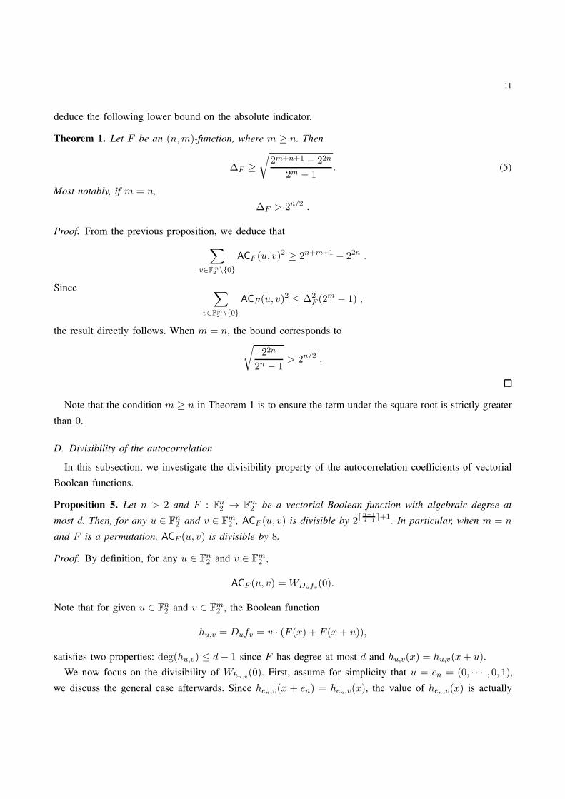
deduce the following lower bound on the absolute indicator.
Theorem 1. Let F be an (n,m)-function, where m ≥ n. Then
∆F ≥
√2m+n+1 − 22n
2m − 1. (5)
Most notably, if m = n,
∆F > 2n/2 .
Proof. From the previous proposition, we deduce that
∑
v∈Fm2 \{0}
ACF (u, v)2 ≥ 2n+m+1 − 22n .
Since ∑
v∈Fm2 \{0}
ACF (u, v)2 ≤ ∆2
F (2m − 1) ,
the result directly follows. When m = n, the bound corresponds to
√22n
2n − 1> 2n/2 .
Note that the condition m ≥ n in Theorem 1 is to ensure the term under the square root is strictly greater
than 0.
D. Divisibility of the autocorrelation
In this subsection, we investigate the divisibility property of the autocorrelation coefficients of vectorial
Boolean functions.
Proposition 5. Let n > 2 and F : Fn2 → F
m2 be a vectorial Boolean function with algebraic degree at
most d. Then, for any u ∈ Fn2 and v ∈ F
m2 , ACF (u, v) is divisible by 2⌈
n−1
d−1⌉+1. In particular, when m = n
and F is a permutation, ACF (u, v) is divisible by 8.
Proof. By definition, for any u ∈ Fn2 and v ∈ F
m2 ,
ACF (u, v) = WDufv(0).
Note that for given u ∈ Fn2 and v ∈ F
m2 , the Boolean function
hu,v = Dufv = v · (F (x) + F (x+ u)),
satisfies two properties: deg(hu,v) ≤ d− 1 since F has degree at most d and hu,v(x) = hu,v(x+ u).
We now focus on the divisibility of Whu,v(0). First, assume for simplicity that u = en = (0, · · · , 0, 1),
we discuss the general case afterwards. Since hen,v(x + en) = hen,v(x), the value of hen,v(x) is actually
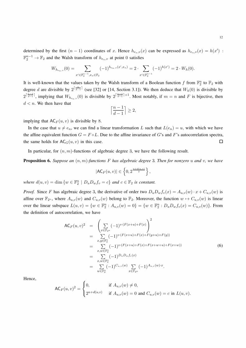
12
determined by the first (n − 1) coordinates of x. Hence hen,v(x) can be expressed as hen,v(x) = h(x′) :
Fn−12 → F2 and the Walsh transform of hen,v at point 0 satisfies
When,v(0) =
∑
x′∈Fn−12 ,xn∈F2
(−1)hen,v(x′,xn) = 2 ·∑
x′∈Fn−12
(−1)h(x′) = 2 ·Wh(0).
It is well-known that the values taken by the Walsh transform of a Boolean function f from Fn2 to F2 with
degree d are divisible by 2⌈n
d−1⌉
(see [32] or [14, Section 3.1]). We then deduce that Wh(0) is divisible by
2⌈n−1
d−1⌉, implying that When,v
(0) is divisible by 2⌈n−1
d−1⌉+1
. Most notably, if m = n and F is bijective, then
d < n. We then have that ⌈n− 1
d− 1
⌉≥ 2,
implying that ACF (u, v) is divisible by 8.
In the case that u 6= en, we can find a linear transformation L such that L(en) = u, with which we have
the affine equivalent function G = F ◦L. Due to the affine invariance of G’s and F ’s autocorrelation spectra,
the same holds for ACG(u, v) in this case.
In particular, for (n,m)-functions of algebraic degree 3, we have the following result.
Proposition 6. Suppose an (n,m)-functions F has algebraic degree 3. Then for nonzero u and v, we have
|ACF (u, v)| ∈{0, 2
n+d(u,v)
2
},
where d(u, v) = dim {w ∈ Fn2 | DuDwfv = c} and c ∈ F2 is constant.
Proof. Since F has algebraic degree 3, the derivative of order two DuDwfv(x) = Au,v(w) · x+Cu,v(w) is
affine over F2n , where Au,v(w) and Cu,v(w) belong to F2. Moreover, the function w 7→ Cu,v(w) is linear
over the linear subspace L(u, v) = {w ∈ Fn2 : Au,v(w) = 0} = {w ∈ F
n2 : DuDwfv(x) = Cu,v(w)}. From
the definition of autocorrelation, we have
ACF (u, v)2 =
(∑
x∈F2n
(−1)v·(F (x+u)+F (x)
)2
=∑
x,y∈Fn2
(−1)v·(F (x+u)+F (x)+F (y+u)+F (y))
=∑
x,w∈Fn2
(−1)v·(F (x+u)+F (x)+F (x+w+u)+F (x+w))
=∑
x,w∈Fn2
(−1)DuDwfv(x)
=∑
w∈Fn2
(−1)Cu,v(w)∑
x∈F2n
(−1)Au,v(w)·x.
(6)
Hence,
ACF (u, v)2 =
0, if Au,v(w) 6= 0,
2n+d(u,v) if Au,v(w) = 0 and Cu,v(w) = c in L(u, v).
13
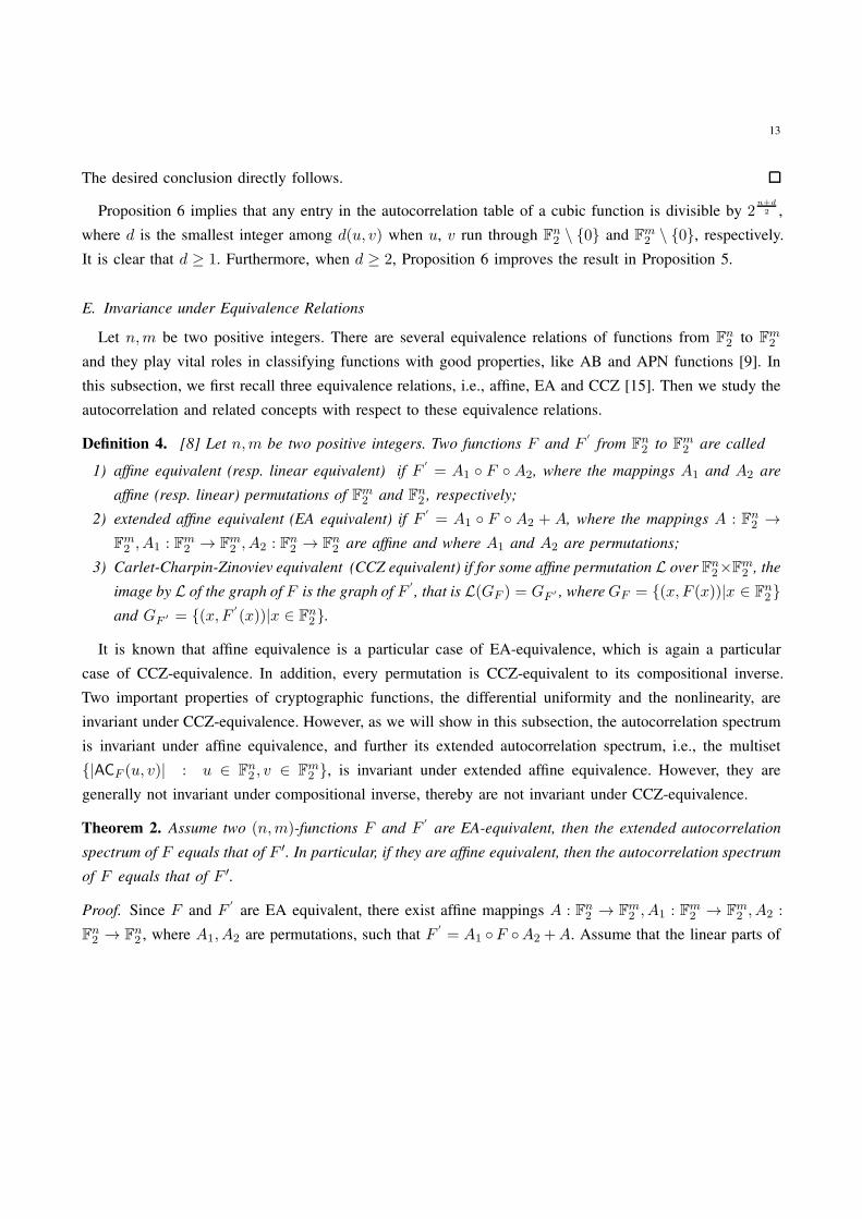
The desired conclusion directly follows.
Proposition 6 implies that any entry in the autocorrelation table of a cubic function is divisible by 2n+d
2 ,
where d is the smallest integer among d(u, v) when u, v run through Fn2 \ {0} and F
m2 \ {0}, respectively.
It is clear that d ≥ 1. Furthermore, when d ≥ 2, Proposition 6 improves the result in Proposition 5.
E. Invariance under Equivalence Relations
Let n,m be two positive integers. There are several equivalence relations of functions from Fn2 to F
m2
and they play vital roles in classifying functions with good properties, like AB and APN functions [9]. In
this subsection, we first recall three equivalence relations, i.e., affine, EA and CCZ [15]. Then we study the
autocorrelation and related concepts with respect to these equivalence relations.
Definition 4. [8] Let n,m be two positive integers. Two functions F and F′
from Fn2 to F
m2 are called
1) affine equivalent (resp. linear equivalent) if F′
= A1 ◦ F ◦ A2, where the mappings A1 and A2 are
affine (resp. linear) permutations of Fm2 and F
n2 , respectively;
2) extended affine equivalent (EA equivalent) if F′
= A1 ◦ F ◦ A2 + A, where the mappings A : Fn2 →
Fm2 , A1 : Fm
2 → Fm2 , A2 : Fn
2 → Fn2 are affine and where A1 and A2 are permutations;
3) Carlet-Charpin-Zinoviev equivalent (CCZ equivalent) if for some affine permutation L over Fn2×F
m2 , the
image by L of the graph of F is the graph of F′
, that is L(GF ) = GF ′ , where GF = {(x, F (x))|x ∈ Fn2}
and GF ′ = {(x, F′
(x))|x ∈ Fn2}.
It is known that affine equivalence is a particular case of EA-equivalence, which is again a particular
case of CCZ-equivalence. In addition, every permutation is CCZ-equivalent to its compositional inverse.
Two important properties of cryptographic functions, the differential uniformity and the nonlinearity, are
invariant under CCZ-equivalence. However, as we will show in this subsection, the autocorrelation spectrum
is invariant under affine equivalence, and further its extended autocorrelation spectrum, i.e., the multiset
{|ACF (u, v)| : u ∈ Fn2 , v ∈ F
m2 }, is invariant under extended affine equivalence. However, they are
generally not invariant under compositional inverse, thereby are not invariant under CCZ-equivalence.
Theorem 2. Assume two (n,m)-functions F and F′
are EA-equivalent, then the extended autocorrelation
spectrum of F equals that of F ′. In particular, if they are affine equivalent, then the autocorrelation spectrum
of F equals that of F ′.
Proof. Since F and F′
are EA equivalent, there exist affine mappings A : Fn2 → F
m2 , A1 : Fm
2 → Fm2 , A2 :
Fn2 → F
n2 , where A1, A2 are permutations, such that F
′
= A1 ◦F ◦A2 +A. Assume that the linear parts of
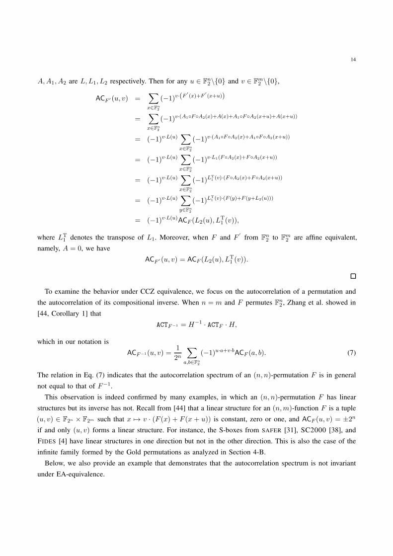
14
A,A1, A2 are L,L1, L2 respectively. Then for any u ∈ Fn2\{0} and v ∈ F
m2 \{0},
ACF ′ (u, v) =∑
x∈Fn2
(−1)v·(F′(x)+F
′(x+u))
=∑
x∈Fn2
(−1)v·(A1◦F◦A2(x)+A(x)+A1◦F◦A2(x+u)+A(x+u))
= (−1)v·L(u)∑
x∈Fn2
(−1)v·(A1◦F◦A2(x)+A1◦F◦A2(x+u))
= (−1)v·L(u)∑
x∈Fn2
(−1)v·L1(F◦A2(x)+F◦A2(x+u))
= (−1)v·L(u)∑
x∈Fn2
(−1)LT1 (v)·(F◦A2(x)+F◦A2(x+u))
= (−1)v·L(u)∑
y∈Fn2
(−1)LT1 (v)·(F (y)+F (y+L2(u)))
= (−1)v·L(u)ACF (L2(u), LT1 (v)),
where LT1 denotes the transpose of L1. Moreover, when F and F
′
from Fn2 to F
m2 are affine equivalent,
namely, A = 0, we have
ACF ′ (u, v) = ACF (L2(u), LT1 (v)).
To examine the behavior under CCZ equivalence, we focus on the autocorrelation of a permutation and
the autocorrelation of its compositional inverse. When n = m and F permutes Fn2 , Zhang et al. showed in
[44, Corollary 1] that
ACTF−1 = H−1 · ACTF ·H,
which in our notation is
ACF−1(u, v) =1
2n
∑
a,b∈Fn2
(−1)u·a+v·bACF (a, b). (7)
The relation in Eq. (7) indicates that the autocorrelation spectrum of an (n, n)-permutation F is in general
not equal to that of F−1.
This observation is indeed confirmed by many examples, in which an (n, n)-permutation F has linear
structures but its inverse has not. Recall from [44] that a linear structure for an (n,m)-function F is a tuple
(u, v) ∈ F2n × F2m such that x 7→ v · (F (x) + F (x + u)) is constant, zero or one, and ACF (u, v) = ±2n
if and only (u, v) forms a linear structure. For instance, the S-boxes from SAFER [31], SC2000 [38], and
FIDES [4] have linear structures in one direction but not in the other direction. This is also the case of the
infinite family formed by the Gold permutations as analyzed in Section 4-B.
Below, we also provide an example that demonstrates that the autocorrelation spectrum is not invariant
under EA-equivalence.
15
Example 1. Let F (x) = 1x ∈ F27 [x] and F
′
(x) = 1x + x. Then F and F
′
are EA-equivalent. However,
ΛF = {−24,−16,−8, 0, 8, 16} while ΛF ′ = {−24,−16,−8, 0, 8, 16, 24}.
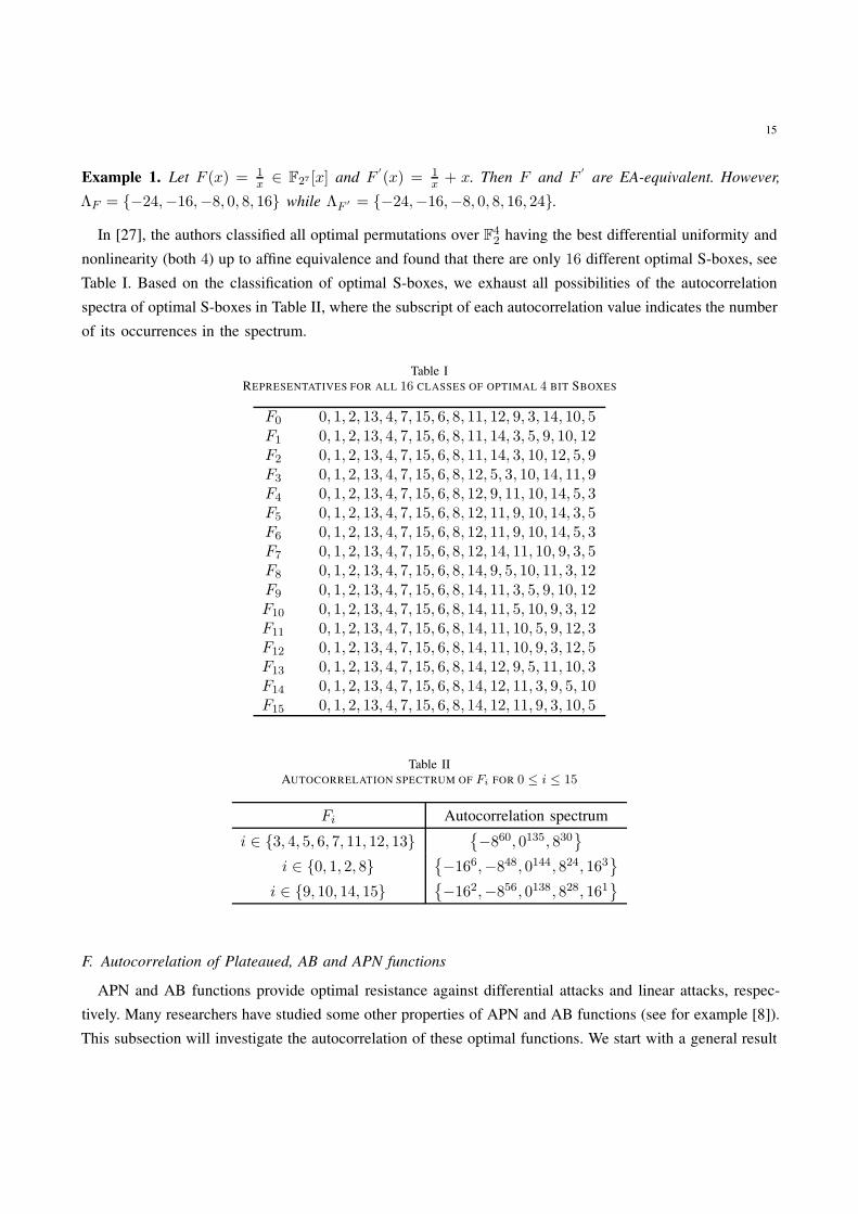
In [27], the authors classified all optimal permutations over F42 having the best differential uniformity and
nonlinearity (both 4) up to affine equivalence and found that there are only 16 different optimal S-boxes, see
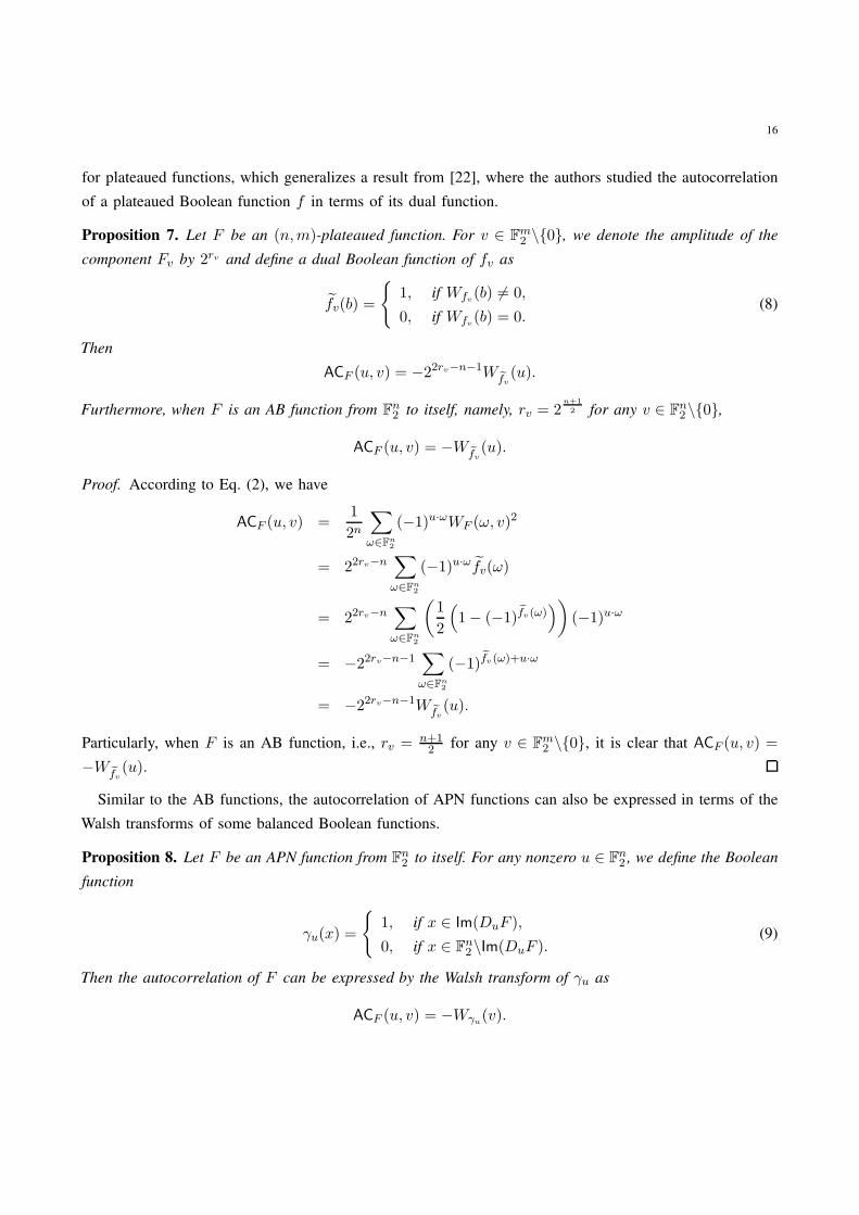
Table I. Based on the classification of optimal S-boxes, we exhaust all possibilities of the autocorrelation
spectra of optimal S-boxes in Table II, where the subscript of each autocorrelation value indicates the number
of its occurrences in the spectrum.
Table I
REPRESENTATIVES FOR ALL 16 CLASSES OF OPTIMAL 4 BIT SBOXES
F0 0, 1, 2, 13, 4, 7, 15, 6, 8, 11, 12, 9, 3, 14, 10, 5F1 0, 1, 2, 13, 4, 7, 15, 6, 8, 11, 14, 3, 5, 9, 10, 12F2 0, 1, 2, 13, 4, 7, 15, 6, 8, 11, 14, 3, 10, 12, 5, 9F3 0, 1, 2, 13, 4, 7, 15, 6, 8, 12, 5, 3, 10, 14, 11, 9F4 0, 1, 2, 13, 4, 7, 15, 6, 8, 12, 9, 11, 10, 14, 5, 3F5 0, 1, 2, 13, 4, 7, 15, 6, 8, 12, 11, 9, 10, 14, 3, 5F6 0, 1, 2, 13, 4, 7, 15, 6, 8, 12, 11, 9, 10, 14, 5, 3F7 0, 1, 2, 13, 4, 7, 15, 6, 8, 12, 14, 11, 10, 9, 3, 5F8 0, 1, 2, 13, 4, 7, 15, 6, 8, 14, 9, 5, 10, 11, 3, 12F9 0, 1, 2, 13, 4, 7, 15, 6, 8, 14, 11, 3, 5, 9, 10, 12F10 0, 1, 2, 13, 4, 7, 15, 6, 8, 14, 11, 5, 10, 9, 3, 12F11 0, 1, 2, 13, 4, 7, 15, 6, 8, 14, 11, 10, 5, 9, 12, 3F12 0, 1, 2, 13, 4, 7, 15, 6, 8, 14, 11, 10, 9, 3, 12, 5F13 0, 1, 2, 13, 4, 7, 15, 6, 8, 14, 12, 9, 5, 11, 10, 3F14 0, 1, 2, 13, 4, 7, 15, 6, 8, 14, 12, 11, 3, 9, 5, 10F15 0, 1, 2, 13, 4, 7, 15, 6, 8, 14, 12, 11, 9, 3, 10, 5
Table II
AUTOCORRELATION SPECTRUM OF Fi FOR 0 ≤ i ≤ 15
Fi Autocorrelation spectrum
i ∈ {3, 4, 5, 6, 7, 11, 12, 13}{−860, 0135, 830
}
i ∈ {0, 1, 2, 8}{−166,−848, 0144, 824, 163
}
i ∈ {9, 10, 14, 15}{−162,−856, 0138, 828, 161
}
F. Autocorrelation of Plateaued, AB and APN functions
APN and AB functions provide optimal resistance against differential attacks and linear attacks, respec-
tively. Many researchers have studied some other properties of APN and AB functions (see for example [8]).
This subsection will investigate the autocorrelation of these optimal functions. We start with a general result
16
for plateaued functions, which generalizes a result from [22], where the authors studied the autocorrelation
of a plateaued Boolean function f in terms of its dual function.
Proposition 7. Let F be an (n,m)-plateaued function. For v ∈ Fm2 \{0}, we denote the amplitude of the
component Fv by 2rv and define a dual Boolean function of fv as
fv(b) =
{1, if Wfv(b) 6= 0,
0, if Wfv(b) = 0.(8)
Then
ACF (u, v) = −22rv−n−1Wfv(u).
Furthermore, when F is an AB function from Fn2 to itself, namely, rv = 2
n+1
2 for any v ∈ Fn2\{0},
ACF (u, v) = −Wfv(u).
Proof. According to Eq. (2), we have
ACF (u, v) =1
2n
∑
ω∈Fn2
(−1)u·ωWF (ω, v)2
= 22rv−n∑
ω∈Fn2
(−1)u·ω fv(ω)
= 22rv−n∑
ω∈Fn2
(1
2
(1− (−1)fv(ω)
))(−1)u·ω
= −22rv−n−1∑
ω∈Fn2
(−1)fv(ω)+u·ω
= −22rv−n−1Wfv(u).
Particularly, when F is an AB function, i.e., rv = n+12 for any v ∈ F
m2 \{0}, it is clear that ACF (u, v) =
−Wfv(u).
Similar to the AB functions, the autocorrelation of APN functions can also be expressed in terms of the
Walsh transforms of some balanced Boolean functions.
Proposition 8. Let F be an APN function from Fn2 to itself. For any nonzero u ∈ F
n2 , we define the Boolean
function
γu(x) =
{1, if x ∈ Im(DuF ),
0, if x ∈ Fn2\Im(DuF ).
(9)
Then the autocorrelation of F can be expressed by the Walsh transform of γu as
ACF (u, v) = −Wγu(v).
17
Proof. Since the APN function F has a 2-to-1 derivative function DuF (x) at any nonzero u, we know that
Im(DuF ) has cardinality 2n−1. Then,
ACF (u, v) =∑
x∈Fn2
(−1)v·(F (x+u)+F (x))
= 2∑
y∈Im(DuF )
(−1)v·y
=∑
y∈Im(DuF )
(−1)v·y −∑
y∈Fn2 \Im(DuF )
(−1)v·y
= −∑
y∈Fn2
(−1)γu(y)+v·y
= −Wγu(v).
From Proposition 8, we see that the autocorrelation of any APN function corresponds to the Walsh
transform of the Boolean function γu in Eq. (9), which is balanced. We then immediately deduce the
following Corollary.
Corollary 1 (Lowest possible absolute indicator for APN functions). Let n be a positive integer. If there
exists an APN function from Fn2 to F
n2 with absolute indicator ∆, then there exists a balanced Boolean
function of n variables with linearity ∆.
To our best knowledge, the smallest known linearity for a balanced function is obtained by Dobbertin’s
recursive construction [20]. For instance, for n = 9, the smallest possible linearity for a balanced Boolean
function is known to belong to the set {24, 28, 32}, which implies that exhibiting an APN function over F92
with absolute indicator 24 would determine the smallest linearity for such a function.
One of the functions whose absolute indicator is known is the inverse mapping F (x) = x2n−2 over F2n .
Proposition 9. [17] The autocorrelation spectrum of the inverse function F (x) = x2n−2 over F2n is given
by
ΛF ={K (v)− 1 + 2× (−1)Tr2n (v) : v ∈ F
∗2n
},
where K(a) =∑
x∈F∗2n(−1)Tr2n(
1
x+ax) is the Kloosterman sum over F2n . Furthermore, the absolute indi-
cator of the inverse function is given by:
i) when n is even, ∆F = 2n
2+1;
ii) when n is odd, ∆F = L(F ) if L(F ) ≡ 0 (mod 8), and ∆F = L(F )± 4 otherwise.
When n is odd, the inverse mapping is APN. Then, from Proposition 8, its autocorrelation table is directly
determined by the corresponding γ. This explains why the absolute indicator of the inverse mapping when
n is odd, is derived from its linearity as detailed in the following example.
18
Example 2 (ACT of the inverse mapping, n odd). For any u ∈ F∗2n , the Boolean function γu, which
characterizes the support of Row u in the DDT of the inverse mapping F : x 7→ x−1, coincides with
(1 + Fu−1) except on two points:
γu(x) =
1 + Tr(u−1x−1) if x 6∈ {0, u−1}
0 if x = 0
1 if x = u−1
.
This comes from the fact that the equation
(x+ u)−1 + x−1 = v
for v 6= u−1 can be rewritten as
x+ (x+ u) = v(x+ u)x
or equivalently when v 6= 0, by setting y = u−1x,
y2 + y = u−1v−1 .
It follows that this equation has two solutions if and only if Tr2n(u−1v−1) = 0. From the proof of the
previous proposition, we deduce
ACF (u, v) = −Wγu(v)
= WFu−1 (v) + 2(1− (−1)Tr2n (u
−1v))
,
where the additional term corresponds to the value of the sum defining the Walsh transform WFu−1 (v) at
points 0 and u−1.
4. AUTOCORRELATION SPECTRA AND ABSOLUTE INDICATOR OF SPECIAL POLYNOMIALS
This section mainly considers some polynomials of special forms. Explicitly, we will investigate the
autocorrelation spectra and the absolute indicator of the Gold permutations and their inverses, and of the
Bracken-Leander functions. Our study is divided into two subsections.
A. Monomials
In the subsection, we consider the autocorrelation of some special monomials of cryptographic interest,
mainly APN permutations and one permutation with differential uniformity 4, over the finite field F2n . Firstly,
we present a general observation on the autocorrelation of monomials.
Proposition 10. Let F (x) = xd ∈ F2n [x]. Then
ΛF = {ACF (1, v) : v ∈ F∗2n} .
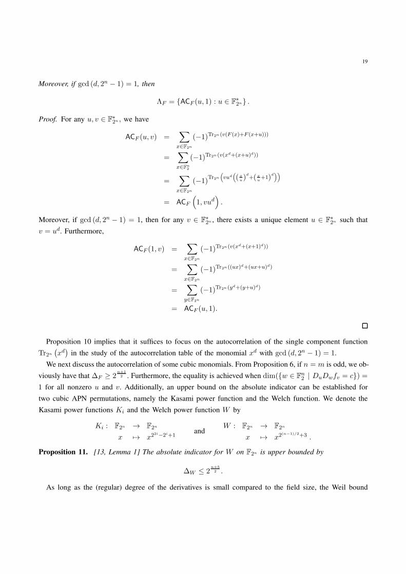
19
Moreover, if gcd (d, 2n − 1) = 1, then
ΛF = {ACF (u, 1) : u ∈ F∗2n} .
Proof. For any u, v ∈ F∗2n , we have
ACF (u, v) =∑
x∈F2n
(−1)Tr2n (v(F (x)+F (x+u)))
=∑
x∈Fn2
(−1)Tr2n (v(xd+(x+u)d))
=∑
x∈F2n
(−1)Tr2n
(vud
(( x
u)d+( x
u+1)
d))
= ACF
(1, vud
).
Moreover, if gcd (d, 2n − 1) = 1, then for any v ∈ F∗2n , there exists a unique element u ∈ F
∗2n such that
v = ud. Furthermore,
ACF (1, v) =∑
x∈F2n
(−1)Tr2n (v(xd+(x+1)d))
=∑
x∈F2n
(−1)Tr2n ((ux)d+(ux+u)d)
=∑
y∈F2n
(−1)Tr2n (yd+(y+u)d)
= ACF (u, 1).
Proposition 10 implies that it suffices to focus on the autocorrelation of the single component function
Tr2n
(xd)
in the study of the autocorrelation table of the monomial xd with gcd (d, 2n − 1) = 1.
We next discuss the autocorrelation of some cubic monomials. From Proposition 6, if n = m is odd, we ob-
viously have that ∆F ≥ 2n+1
2 . Furthermore, the equality is achieved when dim({w ∈ Fn2 | DuDwfv = c}) =
1 for all nonzero u and v. Additionally, an upper bound on the absolute indicator can be established for
two cubic APN permutations, namely the Kasami power function and the Welch function. We denote the
Kasami power functions Ki and the Welch power function W by
Ki : F2n → F2n
x 7→ x22i−2i+1
andW : F2n → F2n
x 7→ x2(n−1)/2+3 .
Proposition 11. [13, Lemma 1] The absolute indicator for W on F2n is upper bounded by
∆W ≤ 2n+5
2 .
As long as the (regular) degree of the derivatives is small compared to the field size, the Weil bound
20
gives a nontrivial upper bound for the absolute indicator of a vectorial Boolean function. This is particularly
interesting for the Kasami functions as the Kasami exponents do not depend on the field size (contrary to
for example the Welch exponent).
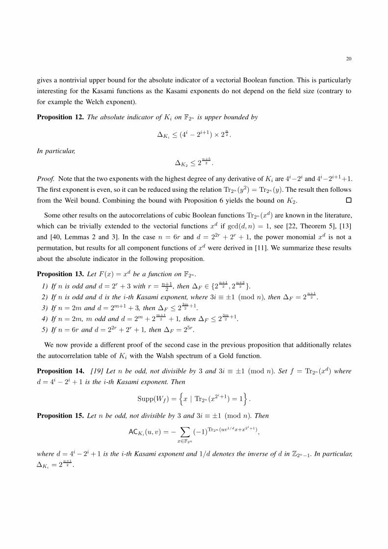
Proposition 12. The absolute indicator of Ki on F2n is upper bounded by
∆Ki≤ (4i − 2i+1)× 2
n
2 .
In particular,
∆K2≤ 2
n+5
2 .
Proof. Note that the two exponents with the highest degree of any derivative of Ki are 4i−2i and 4i−2i+1+1.
The first exponent is even, so it can be reduced using the relation Tr2n(y2) = Tr2n(y). The result then follows
from the Weil bound. Combining the bound with Proposition 6 yields the bound on K2.
Some other results on the autocorrelations of cubic Boolean functions Tr2n(xd) are known in the literature,
which can be trivially extended to the vectorial functions xd if gcd(d, n) = 1, see [22, Theorem 5], [13]
and [40, Lemmas 2 and 3]. In the case n = 6r and d = 22r + 2r + 1, the power monomial xd is not a
permutation, but results for all component functions of xd were derived in [11]. We summarize these results
about the absolute indicator in the following proposition.
Proposition 13. Let F (x) = xd be a function on F2n .
1) If n is odd and d = 2r + 3 with r = n+12 , then ∆F ∈ {2
n+1
2 , 2n+3
2 }.
2) If n is odd and d is the i-th Kasami exponent, where 3i ≡ ±1 (mod n), then ∆F = 2n+1
2 .
3) If n = 2m and d = 2m+1 + 3, then ∆F ≤ 23m
2+1.
4) If n = 2m, m odd and d = 2m + 2m+1
2 + 1, then ∆F ≤ 23m
2+1.
5) If n = 6r and d = 22r + 2r + 1, then ∆F = 25r .
We now provide a different proof of the second case in the previous proposition that additionally relates
the autocorrelation table of Ki with the Walsh spectrum of a Gold function.
Proposition 14. [19] Let n be odd, not divisible by 3 and 3i ≡ ±1 (mod n). Set f = Tr2n(xd) where
d = 4i − 2i + 1 is the i-th Kasami exponent. Then
Supp(Wf ) ={x | Tr2n(x2
i+1) = 1}.
Proposition 15. Let n be odd, not divisible by 3 and 3i ≡ ±1 (mod n). Then
ACKi(u, v) = −
∑
x∈F2n
(−1)Tr2n (uv1/dx+x2i+1),
where d = 4i − 2i +1 is the i-th Kasami exponent and 1/d denotes the inverse of d in Z2n−1. In particular,
∆Ki= 2
n+1
2 .
21
Proof. It is well-known that, if F is a power permutation over a finite field, its Walsh spectrum is uniquely
defined by the entries WF (1, b). Indeed, for v 6= 0,
WKi(u, v) =
∑
x∈F2n
(−1)Tr2n (ux+vxd) =∑
x∈F2n
(−1)Tr2n (uv−1/dx+xd) = WKi
(uv−1/d, 1).
Define a Boolean function
fv(x) =
1, if WKi
(x, v) 6= 0
0, if WKi(x, v) = 0.
By Proposition 14, the function fv becomes
fv(x) = Tr2n((v−1/dx)2i+1).
It follows from Proposition 7 that, for any u and v,
ACKi(u, v) = −Wfv
(u) = −∑
x∈F2n
(−1)Tr2n (ux+(v−1/dx)2i+1) = −
∑
x∈F2n
(−1)Tr2n (uv1/dx+x2i+1).
Observe that gcd(i, n) = 1, so the Gold function x2i+1 is AB and ACKi
= 2n+1
2 .
Note that the cases 3i ≡ 1 (mod n) and 3i ≡ −1 (mod n) are essentially only one case because the i-th
and (n − i)-th Kasami exponents belong to the same cyclotomic coset. Indeed, (4(n−i) − 2n−i + 1)22i ≡
4i − 2i + 1 (mod 2n − 1).
From the known result in the literature, it appears that (n, n)-functions with a low absolute indicator are
rare objects, which is also confirmed by experimental results for small integer n. Below we propose an open
problem for such functions.
Problem 1. For an odd integer n, are there power functions F over F2n with ∆F = 2(n+1)/2 other than
the Kasami APN functions?
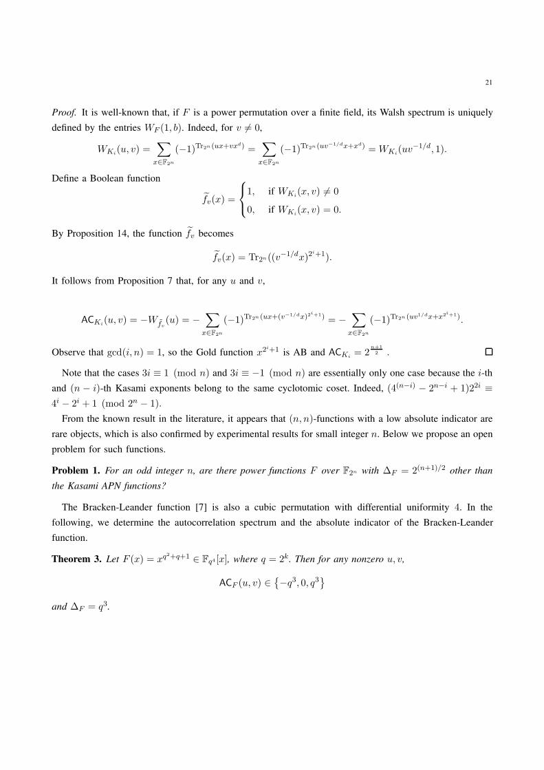
The Bracken-Leander function [7] is also a cubic permutation with differential uniformity 4. In the
following, we determine the autocorrelation spectrum and the absolute indicator of the Bracken-Leander
function.
Theorem 3. Let F (x) = xq2+q+1 ∈ Fq4 [x], where q = 2k. Then for any nonzero u, v,
ACF (u, v) ∈{−q3, 0, q3
}
and ∆F = q3.
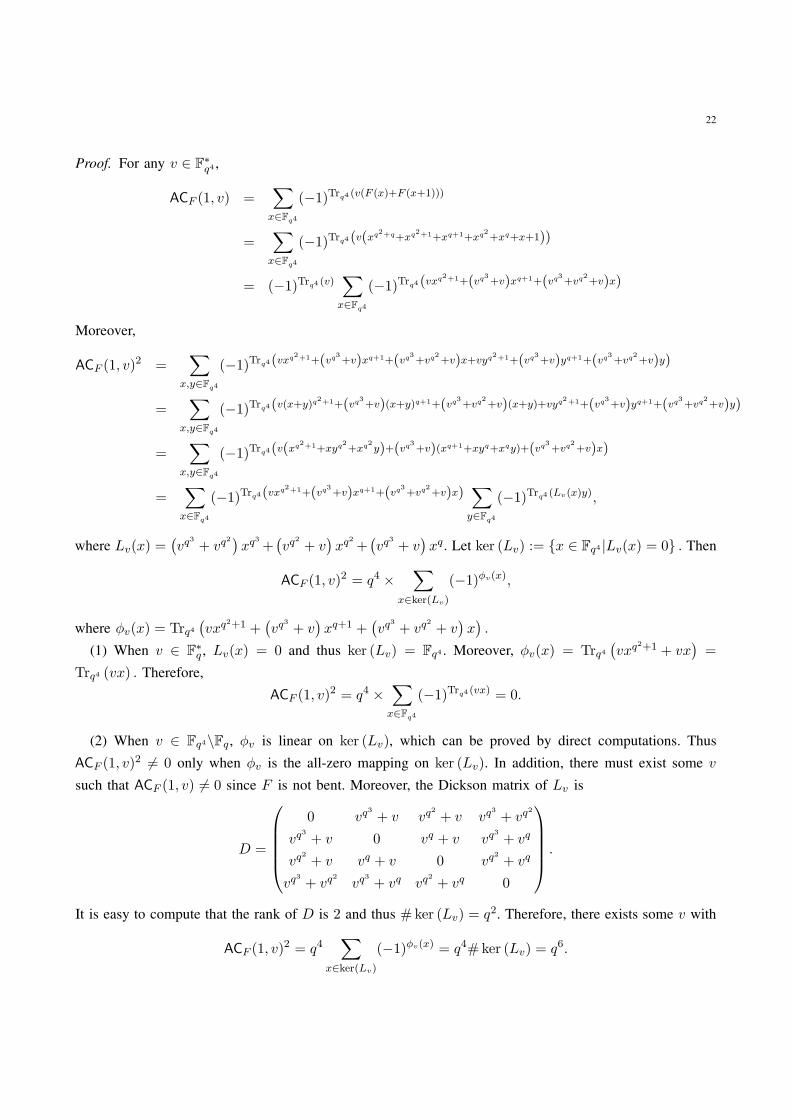
22
Proof. For any v ∈ F∗q4 ,
ACF (1, v) =∑
x∈Fq4
(−1)Trq4 (v(F (x)+F (x+1)))
=∑
x∈Fq4
(−1)Trq4(v(xq2+q+xq2+1+xq+1+xq2+xq+x+1))
= (−1)Trq4 (v)∑
x∈Fq4
(−1)Trq4(vxq2+1+(vq3+v)xq+1+(vq3+vq2+v)x)
Moreover,
ACF (1, v)2 =
∑
x,y∈Fq4
(−1)Trq4(vxq2+1+(vq3+v)xq+1+(vq3+vq2+v)x+vyq2+1+(vq3+v)yq+1+(vq3+vq2+v)y)
=∑
x,y∈Fq4
(−1)Trq4(v(x+y)q2+1+(vq3+v)(x+y)q+1+(vq3+vq2+v)(x+y)+vyq2+1+(vq3+v)yq+1+(vq3+vq2+v)y)
=∑
x,y∈Fq4
(−1)Trq4(v(xq2+1+xyq2+xq2y)+(vq3+v)(xq+1+xyq+xqy)+(vq3+vq2+v)x)
=∑
x∈Fq4
(−1)Trq4(vxq2+1+(vq3+v)xq+1+(vq3+vq2+v)x)
∑
y∈Fq4
(−1)Trq4 (Lv(x)y),
where Lv(x) =(vq
3
+ vq2)
xq3
+(vq
2
+ v)xq
2
+(vq
3
+ v)xq. Let ker (Lv) := {x ∈ Fq4 |Lv(x) = 0} . Then
ACF (1, v)2 = q4 ×
∑
x∈ker(Lv)
(−1)φv(x),
where φv(x) = Trq4(vxq
2+1 +(vq
3
+ v)xq+1 +
(vq
3
+ vq2
+ v)x).
(1) When v ∈ F∗q , Lv(x) = 0 and thus ker (Lv) = Fq4 . Moreover, φv(x) = Trq4
(vxq
2+1 + vx)=
Trq4 (vx) . Therefore,
ACF (1, v)2 = q4 ×
∑
x∈Fq4
(−1)Trq4 (vx) = 0.
(2) When v ∈ Fq4\Fq , φv is linear on ker (Lv), which can be proved by direct computations. Thus
ACF (1, v)2 6= 0 only when φv is the all-zero mapping on ker (Lv). In addition, there must exist some v
such that ACF (1, v) 6= 0 since F is not bent. Moreover, the Dickson matrix of Lv is
D =
0 vq3
+ v vq2
+ v vq3
+ vq2
vq3
+ v 0 vq + v vq3
+ vq
vq2
+ v vq + v 0 vq2
+ vq
vq3
+ vq2
vq3
+ vq vq2
+ vq 0
.
It is easy to compute that the rank of D is 2 and thus #ker (Lv) = q2. Therefore, there exists some v with
ACF (1, v)2 = q4
∑
x∈ker(Lv)
(−1)φv(x) = q4#ker (Lv) = q6.
23
This completes the proof.
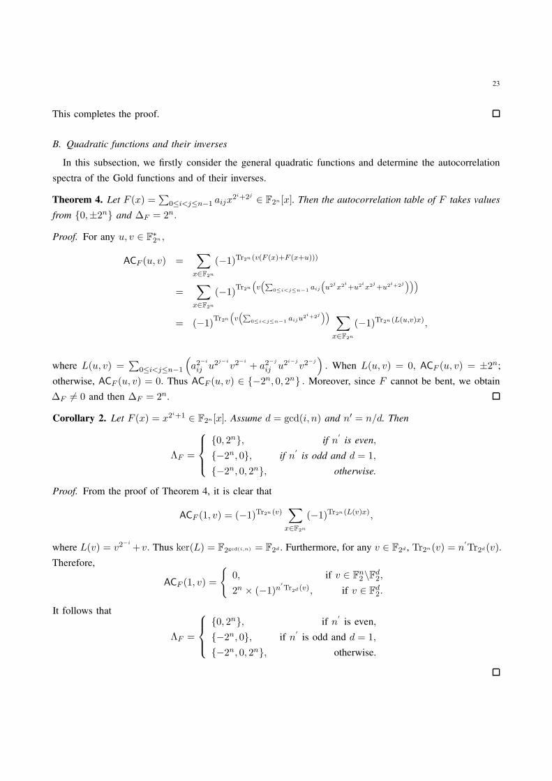
B. Quadratic functions and their inverses
In this subsection, we firstly consider the general quadratic functions and determine the autocorrelation
spectra of the Gold functions and of their inverses.
Theorem 4. Let F (x) =∑
0≤i<j≤n−1 aijx2i+2j
∈ F2n [x]. Then the autocorrelation table of F takes values
from {0,±2n} and ∆F = 2n.
Proof. For any u, v ∈ F∗2n ,
ACF (u, v) =∑
x∈F2n
(−1)Tr2n (v(F (x)+F (x+u)))
=∑
x∈F2n
(−1)Tr2n
(v(∑
0≤i<j≤n−1 aij
(u2jx2i+u2ix2j+u2i+2j
)))
= (−1)Tr2n
(v(∑
0≤i<j≤n−1 aiju2i+2j)) ∑
x∈F2n
(−1)Tr2n (L(u,v)x),
where L(u, v) =∑
0≤i<j≤n−1
(a2
−i
ij u2j−i
v2−i
+ a2−j
ij u2i−j
v2−j). When L(u, v) = 0, ACF (u, v) = ±2n;
otherwise, ACF (u, v) = 0. Thus ACF (u, v) ∈ {−2n, 0, 2n} . Moreover, since F cannot be bent, we obtain
∆F 6= 0 and then ∆F = 2n.
Corollary 2. Let F (x) = x2i+1 ∈ F2n [x]. Assume d = gcd(i, n) and n′ = n/d. Then
ΛF =
{0, 2n}, if n′
is even,
{−2n, 0}, if n′
is odd and d = 1,
{−2n, 0, 2n}, otherwise.
Proof. From the proof of Theorem 4, it is clear that
ACF (1, v) = (−1)Tr2n (v)∑
x∈F2n
(−1)Tr2n (L(v)x),
where L(v) = v2−i
+v. Thus ker(L) = F2gcd(i,n) = F2d . Furthermore, for any v ∈ F2d , Tr2n(v) = n′
Tr2d(v).
Therefore,
ACF (1, v) =
{0, if v ∈ F
n2\F
d2,
2n × (−1)n′Tr2d (v), if v ∈ F
d2.
It follows that
ΛF =
{0, 2n}, if n′
is even,
{−2n, 0}, if n′
is odd and d = 1,
{−2n, 0, 2n}, otherwise.
24
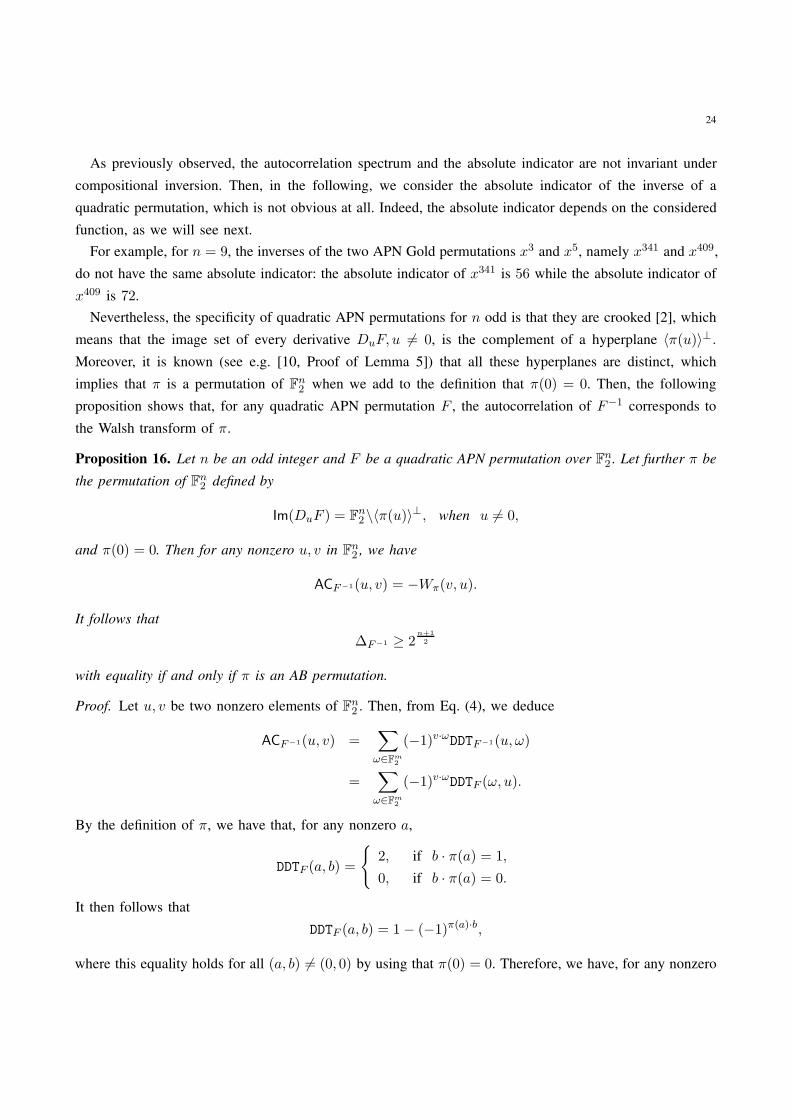
As previously observed, the autocorrelation spectrum and the absolute indicator are not invariant under
compositional inversion. Then, in the following, we consider the absolute indicator of the inverse of a
quadratic permutation, which is not obvious at all. Indeed, the absolute indicator depends on the considered
function, as we will see next.
For example, for n = 9, the inverses of the two APN Gold permutations x3 and x5, namely x341 and x409,
do not have the same absolute indicator: the absolute indicator of x341 is 56 while the absolute indicator of
x409 is 72.
Nevertheless, the specificity of quadratic APN permutations for n odd is that they are crooked [2], which
means that the image set of every derivative DuF, u 6= 0, is the complement of a hyperplane 〈π(u)〉⊥.
Moreover, it is known (see e.g. [10, Proof of Lemma 5]) that all these hyperplanes are distinct, which
implies that π is a permutation of Fn2 when we add to the definition that π(0) = 0. Then, the following
proposition shows that, for any quadratic APN permutation F , the autocorrelation of F−1 corresponds to
the Walsh transform of π.
Proposition 16. Let n be an odd integer and F be a quadratic APN permutation over Fn2 . Let further π be
the permutation of Fn2 defined by
Im(DuF ) = Fn2\〈π(u)〉
⊥, when u 6= 0,
and π(0) = 0. Then for any nonzero u, v in Fn2 , we have
ACF−1(u, v) = −Wπ(v, u).
It follows that
∆F−1 ≥ 2n+1
2
with equality if and only if π is an AB permutation.
Proof. Let u, v be two nonzero elements of Fn2 . Then, from Eq. (4), we deduce
ACF−1(u, v) =∑
ω∈Fm2
(−1)v·ωDDTF−1(u, ω)
=∑
ω∈Fm2
(−1)v·ωDDTF (ω, u).
By the definition of π, we have that, for any nonzero a,
DDTF (a, b) =
{2, if b · π(a) = 1,
0, if b · π(a) = 0.
It then follows that
DDTF (a, b) = 1− (−1)π(a)·b,
where this equality holds for all (a, b) 6= (0, 0) by using that π(0) = 0. Therefore, we have, for any nonzero
25
u and v,
ACF−1(u, v) = −∑
ω∈Fm2
(−1)v·ω(1− (−1)π(ω)·u
)= −Wπ(v, u).
As a consequence, ∆F−1 is equal to the linearity of π, which is at least 2n+1
2 with equality for AB
functions.
It is worth noticing that the previous proposition is valid, not only for quadratic APN permutations, but
for all crooked permutations, which are a particular case of AB functions. However, the existence of crooked
permutations of degree strictly higher than 2 is an open question.
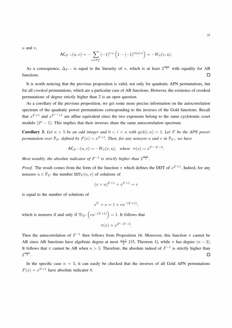
As a corollary of the previous proposition, we get some more precise information on the autocorrelation
spectrum of the quadratic power permutations corresponding to the inverses of the Gold functions. Recall
that x2i+1 and x2
n−i+1 are affine equivalent since the two exponents belong to the same cyclotomic coset
modulo (2n − 1). This implies that their inverses share the same autocorrelation spectrum.
Corollary 3. Let n > 5 be an odd integer and 0 < i < n with gcd(i, n) = 1. Let F be the APN power
permutation over F2n defined by F (x) = x2i+1. Then, for any nonzero u and v in F2n , we have
ACF−1(u, v) = −Wπ(v, u), where π(x) = x2n−2i−2.
Most notably, the absolute indicator of F−1 is strictly higher than 2n+1
2 .
Proof. The result comes from the form of the function π which defines the DDT of x2i+1. Indeed, for any
nonzero u ∈ F2n the number DDTF (u, v) of solutions of
(x+ u)2i+1 + x2
i+1 = v
is equal to the number of solutions of
x2i
+ x = 1 + vu−(2i+1),
which is nonzero if and only if Tr2n
(vu−(2i+1)
)= 1. It follows that
π(x) = x2n−2i−2.
Then the autocorrelation of F−1 then follows from Proposition 16. Moreover, this function π cannot be
AB since AB functions have algebraic degree at most n+12 [15, Theorem 1], while π has degree (n − 2).
It follows that π cannot be AB when n > 5. Therefore, the absolute indeed of F−1 is strictly higher than
2n+1
2 .
In the specific case n = 5, it can easily be checked that the inverses of all Gold APN permutations
F (x) = x2i+1 have absolute indicator 8.
26
5. CONCLUSION
This paper intensively investigates the differential-linear connectivity table (DLCT) of vectorial Boolean
functions. The main contributions of this paper are four-fold. Firstly, we reveal the connection between
DLCT and the autocorrelation table of vectorial Boolean functions and we characterize these two notions in
terms of the Walsh transform of the function and of its differential distribution table. Secondly, we provide
bounds on the absolute indicator of (n,m)-functions when m ≥ n and we exhibit the divisibility property
of the autocorrelation of any vectorial Boolean functions. Moreover, we investigate the invariance of the
autocorrelation table under affine, EA and CCZ equivalence and exhaust the autocorrelation spectra of optimal
4-bit S-boxes. Thirdly, we analyze some properties of the autocorrelation of cryptographically desirable
functions, including APN, plateaued and AB functions and express the autocorrelation of APN and AB
functions with the Walsh transform of certain Boolean functions. Finally, we investigate the autocorrelation
spectra of some special polynomials, including monomials with low differential uniformity, cubic monomials,
quadratic functions and inverses of quadratic permutations.
This paper only covers a small portion of interesting problems on this subject and many problems deserve
further research. For instance, the generic lower bound on the absolute indicator of vectorial Boolean
functions derived in this paper is lower than what experimental results suggest and thus might be further
improved. A natural follow-up topic would be the investigation and construction of optimal, or near-optimal,
vectorial Boolean functions with respect to the bounds.
Note: The current paper is a merged version of [12] and [28].
REFERENCES
[1] Achiya Bar-On, Orr Dunkelman, Nathan Keller, and Ariel Weizman. DLCT: A new tool for differential-linear cryptanalysis.
pages 313–342, 2019.
[2] T.D. Bending and D. Fon-Der-Flaass. Crooked functions, bent functions, and distance regular graphs. The Electronic Journal
of Combinatorics, 5, 1998.
[3] Thierry Berger, Anne Canteaut, Pascale Charpin, and Yann Laigle-Chapuy. On almost perfect nonlinear functions over Fn2 .
IEEE Transactions on Information Theory, 52(9):4160–4170, 2006.
[4] Begül Bilgin, Andrey Bogdanov, Miroslav Kneževic, Florian Mendel, and Qingju Wang. Fides: Lightweight authenticated
cipher with side-channel resistance for constrained hardware. pages 142–158, 2013.
[5] Céline Blondeau and Kaisa Nyberg. New links between differential and linear cryptanalysis. pages 388–404, 2013.
[6] Christina Boura and Anne Canteaut. On the boomerang uniformity of cryptographic sboxes. 2018(3):290–310, 2018.
[7] Carl Bracken and Gregor Leander. A highly nonlinear differentially 4 uniform power mapping that permutes fields of even
degree. Finite Fields and Their Applications, 16(4):231–242, July 2010.
[8] Lilya Budaghyan. Construction and Analysis of Cryptographic Functions. New York, NY, USA: Springer-Verlag, 2014.
[9] Lilya Budaghyan, Claude Carlet, and Alex Pott. New classes of almost bent and almost perfect nonlinear polynomials. IEEE
Transactions on Information Theory, 52(3):1141–1152, March 2006.
[10] Anne Canteaut and Pascale Charpin. Decomposing bent functions. IEEE Transactions on Information Theory, 49(8):2004–2019,
Aug. 2003.
[11] Anne Canteaut, Pascale Charpin, and Gohar M. Kyureghyan. A new class of monomial bent functions. Finite Fields and
Their Applications, 14(1):221–241, Jan. 2008.
27
[12] Anne Canteaut, Lukas Kölsch, and Friedrich Wiemer. Observations on the DLCT and absolute indicators. Cryptology ePrint
Archive, https://eprint.iacr.org/2019/848.pdf, 2019.
[13] Claude Carlet. Recursive lower bounds on the nonlinearity profile of boolean functions and their applications. IEEE Transactions
on Information Theory, 54(3):1262–1272, March 2008.
[14] Claude Carlet. Boolean functions for cryptography and error-correcting codes. In Yves Crama and Peter L. Hammer, editors,
Boolean Models and Methods in Mathematics, Computer Science, and Engineering, pages 257–397. Cambridge University
Press, 2010.
[15] Claude Carlet, Pascale Charpin, and Victor Zinoviev. Codes, bent functions and permutations suitable for DES-like
cryptosystems. Designs, Codes and Cryptography, 15(2):125–156, 1998.
[16] Florent Chabaud and Serge Vaudenay. Links between differential and linear cryptanalysis. pages 356–365, 1995.
[17] Pascale Charpin, Tor Helleseth, and Victor Zinoviev. Propagation characteristics of x 7→ x−1 and Kloosterman sums. Finite
Fields and Their Applications, 13(2):366–381, April 2007.
[18] Carlos Cid, Tao Huang, Thomas Peyrin, Yu Sasaki, and Ling Song. Boomerang connectivity table: A new cryptanalysis tool.
pages 683–714, 2018.
[19] John F. Dillon. Multiplicative difference sets via additive characters. Designs, Codes and Cryptography, 17(1-3):225–235,
1999.
[20] Hans Dobbertin. Construction of Bent functions and balanced Boolean functions with high nonlinearity. pages 61–74, 1995.
[21] Sugata Gangopadhyay, Pradipkumar H. Keskar, and Subhamoy Maitra. Patterson-Wiedemann construction revisited. Discrete
Mathematics, 306(14):1540–1556, 2006.
[22] Guang Gong and Khoongming Khoo. Additive autocorrelation of resilient Boolean functions. pages 275–290, 2004.
[23] Selçuk Kavut. Correction to the paper: Patterson-Wiedemann construction revisited. Discrete Applied Mathematics, 202:185–
187, 2016.
[24] Selçuk Kavut, Subhamoy Maitra, and Deng Tang. Construction and search of balanced boolean functions on even number of
variables towards excellent autocorrelation profile. Des. Codes Cryptogrography, 87(2–3):261–276, 2019.
[25] Selçuk Kavut, Subhamoy Maitra, and Melek D. Yücel. Search for boolean functions with excellent profiles in the rotation
symmetric class. IEEE Trans. Information Theory, 53(5):1743–1751, 2007.
[26] Susan K. Langford and Martin E. Hellman. Differential-linear cryptanalysis. pages 17–25, 1994.
[27] Gregor Leander and Axel Poschmann. On the classification of 4 bit S-boxes. In Arithmetic of Finite Fields, pages 159–176.
Springer Berlin Heidelberg, 2007.
[28] Kangquan Li, Chunlei Li, Chao Li, and Longjiang Qu. On the differential-linear connectivity table of vectorial boolean
functions. CoRR., http://arxiv.org/abs/1907.05986, 2019.
[29] Kangquan Li, Longjiang Qu, Bing Sun, and Chao Li. New results about the boomerang uniformity of permutation polynomials.
IEEE Transactions on Information Theory, 2019.
[30] Subhamoy Maitra and Palash Sarkar. Modifications of Patterson-Wiedemann functions for cryptographic applications. IEEE
Trans. Information Theory, 48(1):278–284, 2002.
[31] James L. Massey. SAFER K-64: A byte-oriented block-ciphering algorithm. pages 1–17, 1994.
[32] Robert J. McEliece. Weight congruences for p-ary cyclic codes. Discrete Mathematics, 3(1-3):177–192, 1972.
[33] Sihem Mesnager. Bent Functions: Fundamentals and Results. Springer International Publishing, 2016.
[34] Sihem Mesnager, Chunming Tang, and Maosheng Xiong. On the boomerang uniformity of (quadratic) permutations over F2n .
CoRR, 2019.
[35] Kaisa Nyberg. Differentially uniform mappings for cryptography. pages 55–64, 1994.
[36] Kaisa Nyberg. S-boxes and round functions with controllable linearity and differential uniformity. pages 111–130, 1995.
[37] Oscar S. Rothaus. On “bent” functions. Journal of Combinatorial Theory, Series A, 20(3):300–305, May 1976.
[38] Takeshi Shimoyama, Hitoshi Yanami, Kazuhiro Yokoyama, Masahiko Takenaka, Kouichi Itoh, Jun Yajima, Naoya Torii, and
Hidema Tanaka. The block cipher SC2000. pages 312–327, 2002.
[39] Ling Song, Xianrui Qin, and Lei Hu. Boomerang connectivity table revisited. 2019(1):118–141, 2019.
28
[40] Guanghong Sun and Chuankun Wu. The lower bound on the second-order nonlinearity of a class of boolean functions with
high nonlinearity. Applicable Algebra in Engineering, Communication and Computing, 22(1):37–45, Dec. 2009.
[41] Deng Tang and Subhamoy Maitra. Construction of n-variable (n ≡ 2 mod 4) balanced boolean functions with maximum
absolute value in autocorrelation spectra < 2n/2. IEEE Trans. Information Theory, 64(1):393–402, 2018.
[42] Natalia Tokareva. Bent Functions: Results and Applications to Cryptography. Academic Press, 2015.
[43] Xian-Mo Zhang and Yuliang Zheng. GAC — the criterion for global avalanche characteristics of cryptographic functions. In
J.UCS The Journal of Universal Computer Science, pages 320–337. Springer Berlin Heidelberg, 1996.
[44] Xian-Mo Zhang, Yuliang Zheng, and Hideki Imai. Relating differential distribution tables to other properties of of substitution
boxes. Designs, Codes and Cryptography, 19(1):45–63, 2000.