Embed Size (px)
Citation preview
1
On the Difference of Effect on Energy Consumption between
Energy Tax and Pre-Tax Energy Price: An International Panel-Data Analysis on
Gasoline Demand
Park Seung-Joon
4. Nov. 2010GCET 2010, Bangkok, Thailand
2
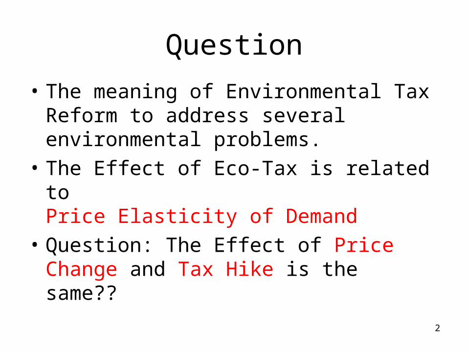
Question
• The meaning of Environmental Tax Reform to address several environmental problems.
• The Effect of Eco-Tax is related to Price Elasticity of Demand
• Question: The Effect of Price Change and Tax Hike is the same??
3
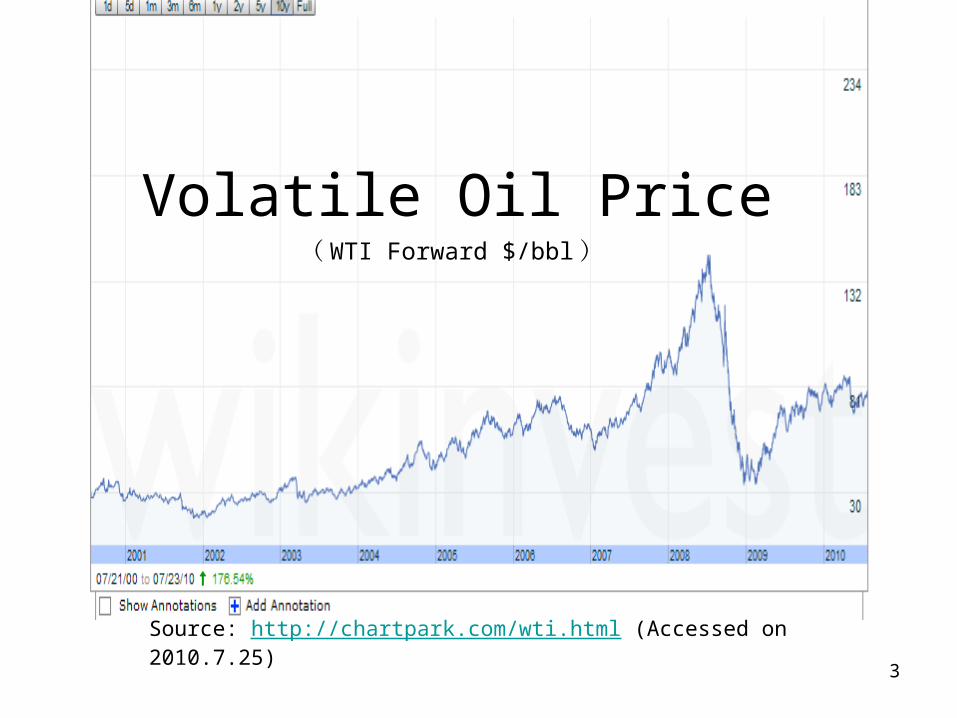
Volatile Oil Price
Source: http://chartpark.com/wti.html (Accessed on 2010.7.25)
( WTI Forward $/bbl )
4
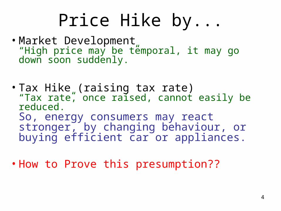
Price Hike by...• Market Development
“High price may be temporal, it may go down soon suddenly.”
• Tax Hike (raising tax rate)“Tax rate, once raised, cannot easily be reduced.”So, energy consumers may react stronger, by changing behaviour, or buying efficient car or appliances.
• How to Prove this presumption??
5
Existing Study
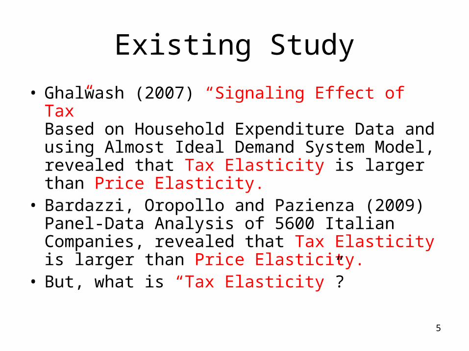
• Ghalwash (2007) “Signaling Effect of Tax”Based on Household Expenditure Data and using Almost Ideal Demand System Model, revealed that Tax Elasticity is larger than Price Elasticity.
• Bardazzi, Oropollo and Pazienza (2009) Panel-Data Analysis of 5600 Italian Companies, revealed that Tax Elasticity is larger than Price Elasticity.
• But, what is “Tax Elasticity”?
6
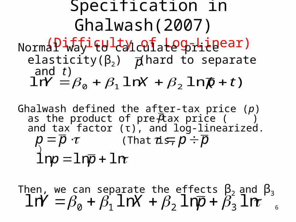
Specification in Ghalwash(2007) (Difficulty of Log-Linear)
Normal way to calculate price elasticity(β2) (hard to separate and t)
Ghalwash defined the after-tax price (p) as the product of pre-tax price ( ) and tax factor (τ), and log-linearized.
(That is, )
Then, we can separate the effects β2 and β3
)ln(lnln 210 tpXY
pp
lnlnln pp
pp
lnlnlnln 3210 pXY
p
p
7
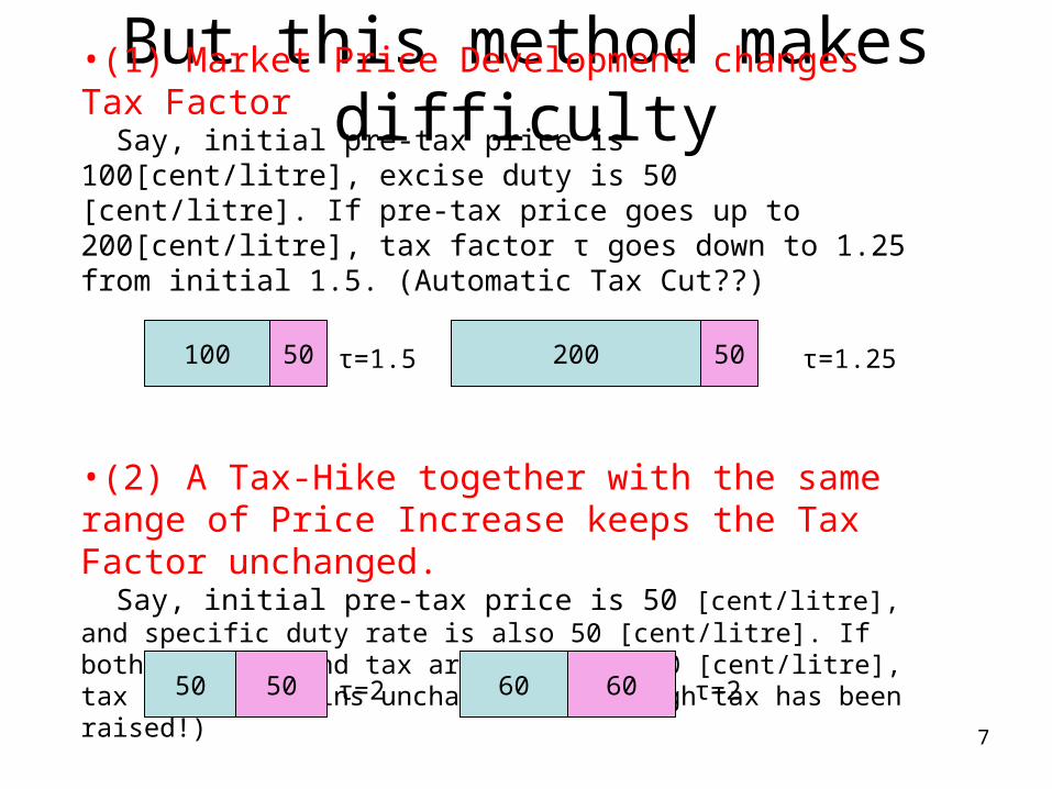
But this method makes difficulty•(1) Market Price Development changes Tax Factor Say, initial pre-tax price is 100[cent/litre], excise duty is 50 [cent/litre]. If pre-tax price goes up to 200[cent/litre], tax factor τ goes down to 1.25 from initial 1.5. (Automatic Tax Cut??)
•(2) A Tax-Hike together with the same range of Price Increase keeps the Tax Factor unchanged. Say, initial pre-tax price is 50 [cent/litre], and specific duty rate is also 50 [cent/litre]. If both of price and tax are raised by 10 [cent/litre], tax factor remains unchanged. (Although tax has been raised!)
100 50 200 50τ=1.5 τ=1.25
50 50 τ=2 60 60 τ=2
8
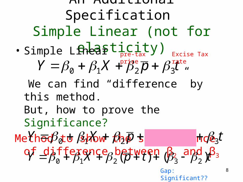
An Additional Specification Simple Linear (not for elasticity)
• Simple Linear
We can find “difference” by this method.But, how to prove the Significance?
Method to show the significance of difference between β2 and β3
tpXY 3210
tttpXY 322210
ttpXY )()( 23210 Gap: Significant??
pre-tax price Excise Tax rate
9
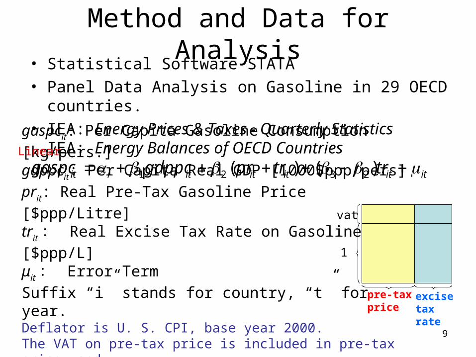
Method and Data for Analysis• Statistical Software STATA• Panel Data Analysis on Gasoline in 29 OECD countries.• IEA: Energy Prices & Taxes - Quarterly Statistics
IEA: Energy Balances of OECD Countries
itititititiit trtrprgdppcgaspc )()( 2321gaspcit: Per Capita Gasoline Consumption [kg/pers.]gdppcit: Per Capita Real GDP [1000$ppp/pers]prit: Real Pre-Tax Gasoline Price [$ppp/Litre]trit : Real Excise Tax Rate on Gasoline [$ppp/L]μit : Error TermSuffix “i” stands for country, “t” for year.Deflator is U. S. CPI, base year 2000.The VAT on pre-tax price is included in pre-tax price, and the VAT on excise tax rate is included in the excise tax rate.
1
vat
pre-taxprice
excise tax rate
Linear
10
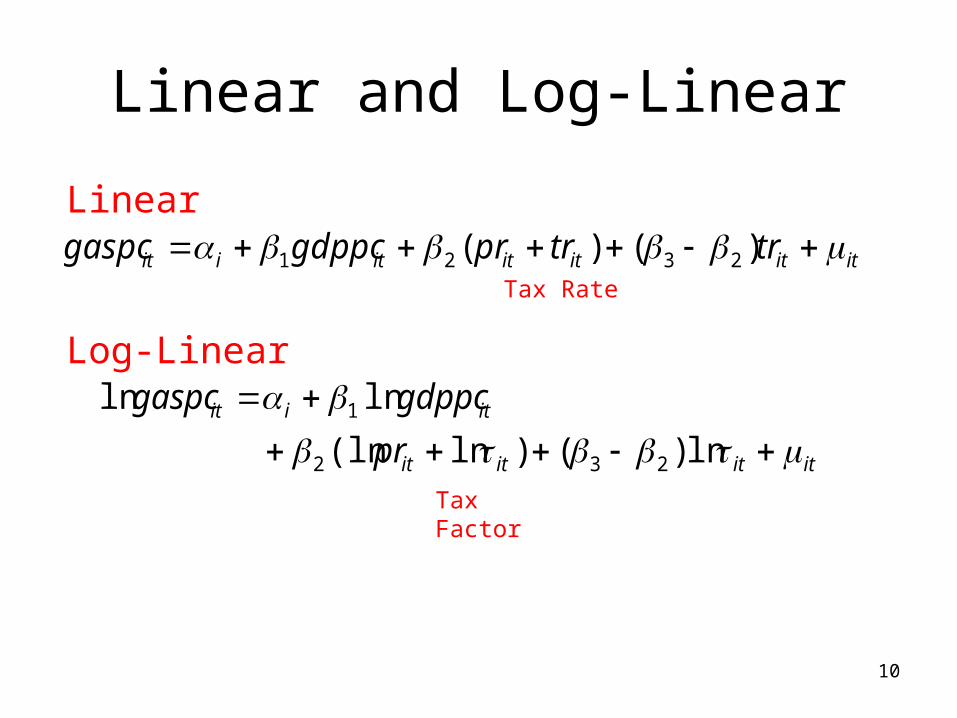
Linear and Log-Linear
itititititiit trtrprgdppcgaspc )()( 2321
Linear
itititit
itiit
pr
gdppcgaspc
ln)()ln(ln
lnln
232
1
Log-Linear
Tax Factor
Tax Rate
11
05
001
000
150
0g
asp
c
15 20 25 30 35 40gdppc
Australia France
Germany ItalyJapan KoreaUnited Kingdom United States
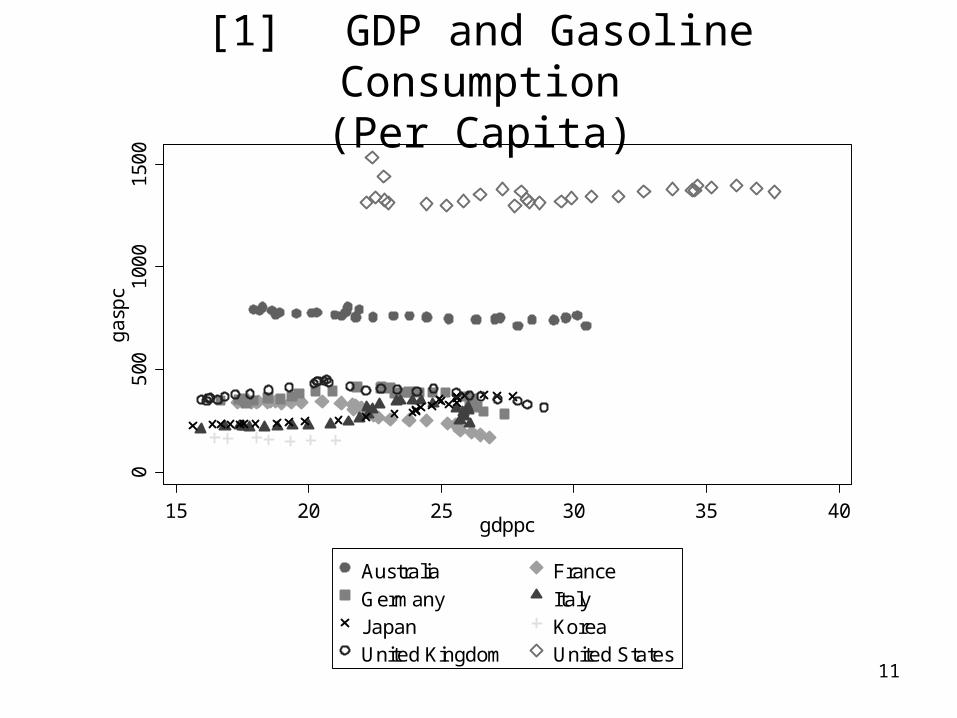
[1] GDP and Gasoline Consumption(Per Capita)
12
05
001
000
150
0g
asp
c
0 .5 1 1.5 2 2.5trpr
Australia France
Germany ItalyJapan KoreaUnited Kingdom United States
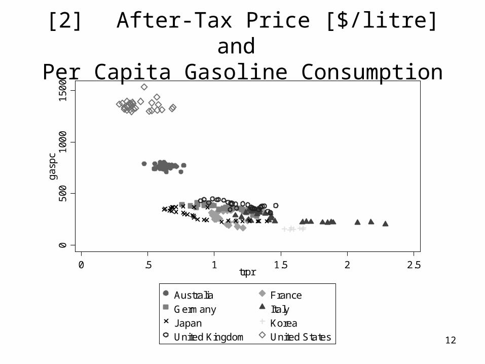
[2] After-Tax Price [$/litre] and Per Capita Gasoline Consumption
13
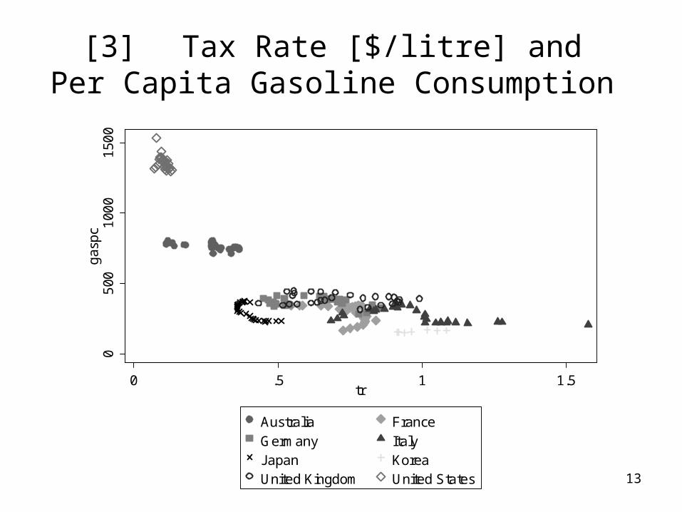
[3] Tax Rate [$/litre] and Per Capita Gasoline Consumption
05
001
000
150
0g
asp
c
0 .5 1 1.5tr
Australia France
Germany ItalyJapan KoreaUnited Kingdom United States
Panel Data Analysis
14
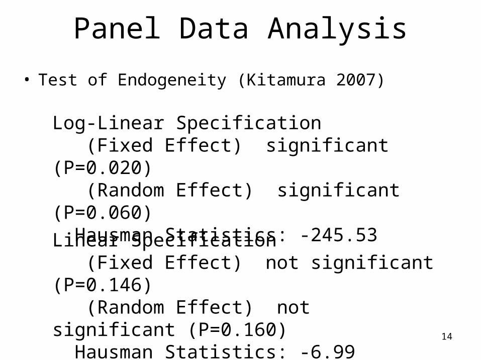
• Test of Endogeneity (Kitamura 2007)
Log-Linear Specification (Fixed Effect) significant (P=0.020) (Random Effect) significant (P=0.060) Hausman Statistics: -245.53
Linear Specification (Fixed Effect) not significant (P=0.146) (Random Effect) not significant (P=0.160) Hausman Statistics: -6.99
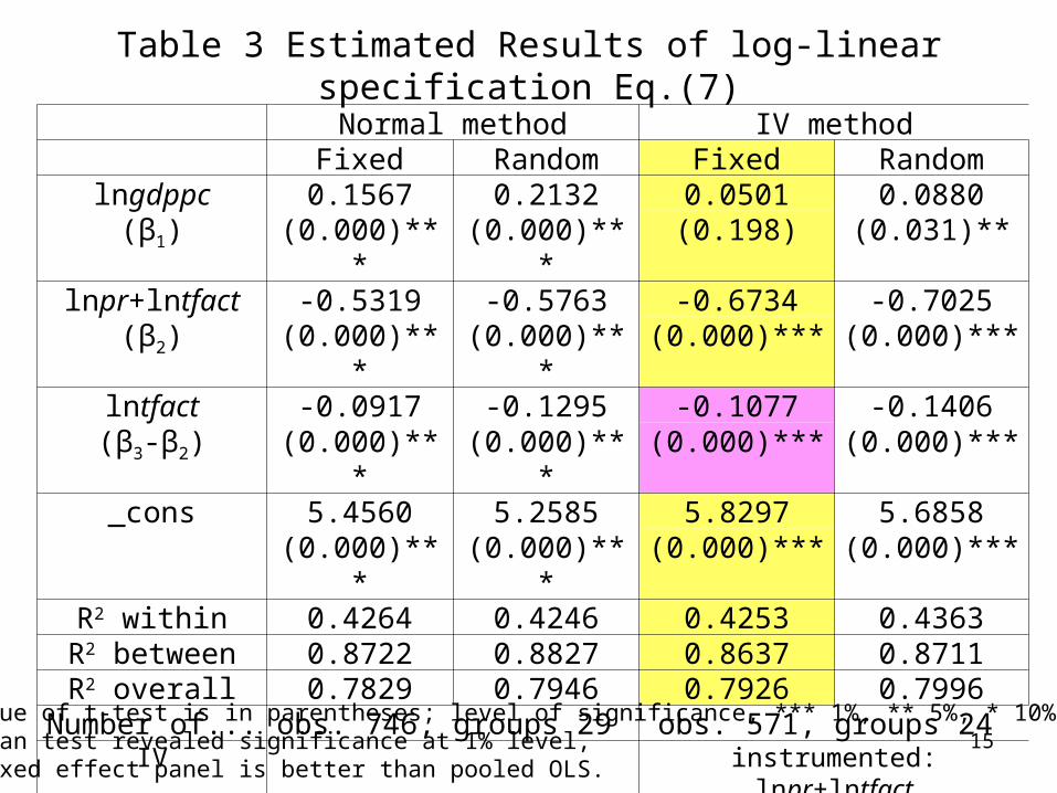
Table 3 Estimated Results of log-linear specification Eq.(7)
15
Normal method IV method Fixed Random Fixed Random
lngdppc 0.1567 0.2132 0.0501 0.0880(β1) (0.000)*** (0.000)*** (0.198) (0.031)**
lnpr+lntfact -0.5319 -0.5763 -0.6734 -0.7025(β2) (0.000)*** (0.000)*** (0.000)*** (0.000)***
lntfact -0.0917 -0.1295 -0.1077 -0.1406(β3-β2) (0.000)*** (0.000)*** (0.000)*** (0.000)***_cons 5.4560 5.2585 5.8297 5.6858
(0.000)*** (0.000)*** (0.000)*** (0.000)***R2 within 0.4264 0.4246 0.4253 0.4363
R2 between 0.8722 0.8827 0.8637 0.8711R2 overall 0.7829 0.7946 0.7926 0.7996
Number of... obs. 746, groups 29 obs. 571, groups 24 IV
instrumented: lnpr+lntfact
instruments: lngdppc lntfact lnpcorHausman Stat. -212.00 44.35 (p=0.000)***
Note: p-Value of t-test is in parentheses; level of significance, *** 1%, ** 5%, * 10%.Breusch-Pagan test revealed significance at 1% level, implying fixed effect panel is better than pooled OLS.
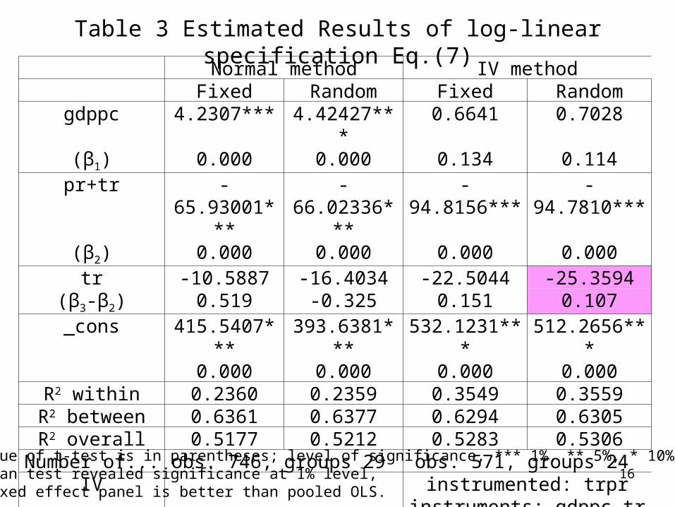
Table 3 Estimated Results of log-linear specification Eq.(7)
16
Normal method IV method Fixed Random Fixed Random
gdppc 4.2307*** 4.42427*** 0.6641 0.7028(β1) 0.000 0.000 0.134 0.114
pr+tr -65.93001*** -66.02336*** -94.8156*** -94.7810***(β2) 0.000 0.000 0.000 0.000tr -10.5887 -16.4034 -22.5044 -25.3594
(β3-β2) 0.519 -0.325 0.151 0.107_cons 415.5407*** 393.6381*** 532.1231*** 512.2656***
0.000 0.000 0.000 0.000R2 within 0.2360 0.2359 0.3549 0.3559
R2 between 0.6361 0.6377 0.6294 0.6305R2 overall 0.5177 0.5212 0.5283 0.5306
Number of... obs. 746, groups 29 obs. 571, groups 24 IV
instrumented: trpr
instruments: gdppc tr pcorHausman Stat. -20.71 -29.95Note: p-Value of t-test is in parentheses; level of significance, *** 1%, ** 5%, * 10%.Breusch-Pagan test revealed significance at 1% level, implying fixed effect panel is better than pooled OLS.
17
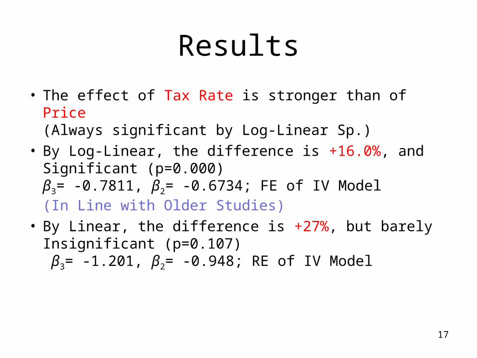
Results
• The effect of Tax Rate is stronger than of Price(Always significant by Log-Linear Sp.)
• By Log-Linear, the difference is +16.0%, and Significant (p=0.000)β3= -0.7811, β2= -0.6734; FE of IV Model(In Line with Older Studies)
• By Linear, the difference is +27%, but barely Insignificant (p=0.107) β3= -1.201, β2= -0.948; RE of IV Model
18
LiteratureBardazzi, R, F. Oropallo and M. G. Pazienza (2009) “Industrial CO2
emissions in Italy: a microsimulation analysis of Environmental Taxes on Firm’s Energy Demand” Critical Issues in Environmental Taxation IV
Ghalwash, T. (2007) “Energy Taxes as a Signaling Device: An Empirical Analysis of Consumer Preferences” Energy Policy, Vol. 35, Issue 1, p. 29-38
Schreiber, S. (2008) The Hausman Test Statistics can be Negative even Asymptotically, Journal of Economics and Statistics (Jahrbuecher fuer Nationaloekonomie und Statistik), 2008, vol. 228, issue 4, pages 394-405
Kitamura (2007) 北村行伸『パネルデータ分析』岩波書店Tsutsui et al. (2008) 筒井淳也・平井裕久・秋吉美都・水落正明・
坂本和靖・福田亘孝 (2007) 『 Stata で計量経済学入門』ミネルヴァ書房
19
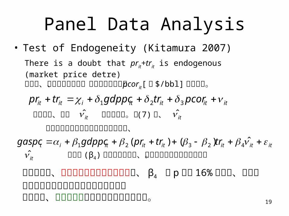
Panel Data Analysis• Test of Endogeneity (Kitamura 2007)
There is a doubt that prit+trit is endogenous (market price detre)そこで、操作変数として、実質輸入原油費用 pcorit[ 米 $/bbl]を用いる。
ititititiitit pcortrgdppctrpr 321
を推定し、残差 it̂ を計算する。式 (7) に、it̂を説明変数として含めることによって、
ititititititit trtrprgdppcgaspc ˆ)()( 42321
it̂の係数 (β4) が有意であれば、内生性があると見なされる。
検定の結果、内生性は無いと判定されたが、 β4 の p 値は 16% 程度で、高くない(内生性が無いことを断定し難い)。そのため、操作変数法も用いて結果を比較する。