1 of 33 © 2014 Pearson Education, Inc. CHAPTER OUTLINE 8 Aggregate Expenditure and Equilibrium Output The Keynesian Theory of Consumption Other Determinants

1 of 33© 2014 Pearson Education, Inc.

CHAPTER OUTLINE

8Aggregate Expenditure and

Equilibrium Output

The Keynesian Theory of Consumption Other Determinants of Consumption

Planned Investment (I) versus Actual InvestmentPlanned Investment and the Interest Rate (r)

Other Determinants of Planned Investment

The Determination of Equilibrium Output (Income) The Saving/Investment Approach to Equilibrium

Adjustment to Equilibrium

The MultiplierThe Multiplier Equation

Looking AheadAppendix: Deriving the Multiplier Algebraically


aggregate output The total quantity of goods and services produced (or supplied) in an economy in a given period.

aggregate income The total income received by all factors of production in a given period.

In any given period, there is an exact equality between aggregate output (production) and aggregate income. You should be reminded of this fact whenever you encounter the combined term aggregate output (income) (Y).

aggregate output (income) (Y) A combined term used to remind you of the exact equality between aggregate output and aggregate income.

From the outset, you must think in “real terms.” Output Y refers to the quantities of goods and services produced, not the dollars circulating in the economy.

Also, we are taking as fixed for purposes of this chapter and the next the interest rate (r) and the overall price level (P).


consumption function The relationship between consumption and income.

FIGURE 8.1 A Consumption Function for a Household

A consumption function for an individual household shows the level of consumption at each level of household income.

The Keynesian Theory of Consumption


With a straight line consumption curve, we can use the following equation to describe the curve:

FIGURE 8.2 An Aggregate Consumption Function

The aggregate consumption function shows the level of aggregate consumption at each level of aggregate income.The upward slope indicates that higher levels of income lead to higher levels of consumption spending.

C = a + bY


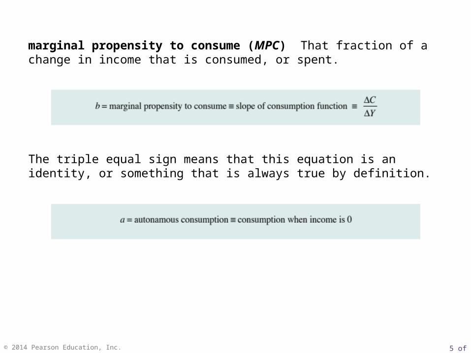
marginal propensity to consume (MPC) That fraction of a change in income that is consumed, or spent.

The triple equal sign means that this equation is an identity, or something that is always true by definition.


aggregate saving (S) The part of aggregate income that is not consumed.

S ≡ Y – C


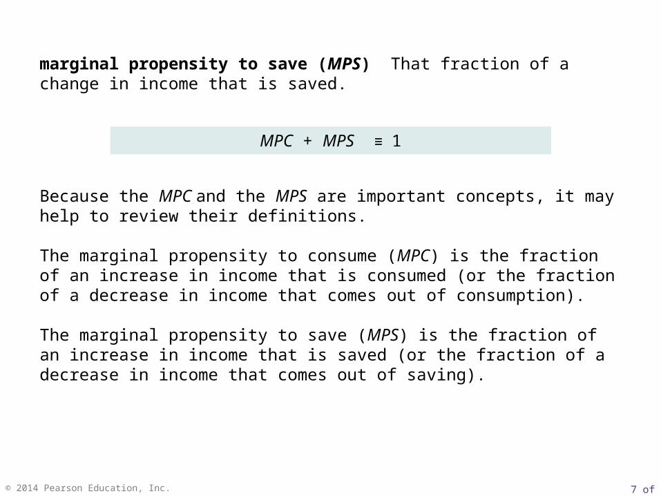
marginal propensity to save (MPS) That fraction of a change in income that is saved.

MPC + MPS ≡ 1

Because the MPC and the MPS are important concepts, it may help to review their definitions.

The marginal propensity to consume (MPC) is the fraction of an increase in income that is consumed (or the fraction of a decrease in income that comes out of consumption).

The marginal propensity to save (MPS) is the fraction of an increase in income that is saved (or the fraction of a decrease in income that comes out of saving).


FIGURE 8.3 The Aggregate Consumption Function Derived from the Equation C = 100 + .75Y In this simple consumption function, consumption is 100 at an income of zero.As income rises, so does consumption. For every 100 increase in income, consumption rises by 75. The slope of the line is .75.

Aggregate Income, Y

Aggregate Consumption, C

0 100

80 160

100 175

200 250

400 400

600 550

800 700

1,000 850


FIGURE 8.4 Deriving the Saving Function from the Consumption Function in Figure 8.3

Because S ≡ Y – C, it is easy to derive the saving function from the consumption function. A 45° line drawn from the origin can be used as a convenient tool to compare consumption and income graphically.At Y = 200, consumption is 250. The 45° line shows us that consumption is larger than income by 50. Thus, S ≡ Y – C = 50.At Y = 800, consumption is less than income by 100. Thus, S = 100 when Y = 800.

Y AGGREGATE

INCOME

C

AGGREGATE CONSUMPTION

= S

AGGREGATE SAVING

0 100 -100

80 160 -80

100 175 -75

200 250 -50

400 400 0

600 550 50

800 700 100

1,000 850 150


The assumption that consumption depends only on income is obviously a simplification.

In practice, the decisions of households on how much to consume in a given period are also affected by their wealth, by the interest rate, and by their expectations of the future.

Households with higher wealth are likely to spend more, other things being equal, than households with less wealth.

Lower interest rates are likely to stimulate spending.

If households are optimistic and expect to do better in the future, they may spend more at present than if they think the future will be bleak.

Other Determinants of Consumption


Planned Investment (I) versus Actual Investment

planned investment (I) Those additions to capital stock and inventory that are planned by firms.

actual investment The actual amount of investment that takes place; it includes items such as unplanned changes in inventories.

A firm’s inventory is the stock of goods that it has awaiting sale.

If a firm overestimates how much it will sell in a period, it will end up with more in inventory than it planned to have.

We will use I to refer to planned investment, not necessarily actual investment.


FIGURE 8.5 Planned Investment Schedule

Planned investment spending is a negative function of the interest rate. An increase in the interest rate from 3 percent to 6 percent reduces planned investment from I0 to I1.

Planned Investment and the Interest Rate (r)

Increasing the interest rate, ceteris paribus, is likely to reduce the level of planned investment spending. When the interest rate falls, it becomes less costly to borrow and more investment projects are likely to be undertaken.


The decision of a firm on how much to invest depends on, among other things, its expectation of future sales.

The optimism or pessimism of entrepreneurs about the future course of the economy can have an important effect on current planned investment. Keynes used the phrase animal spirits to describe the feelings of entrepreneurs.

For now, we will assume that planned investment simply depends on the interest rate.

Other Determinants of Planned Investment


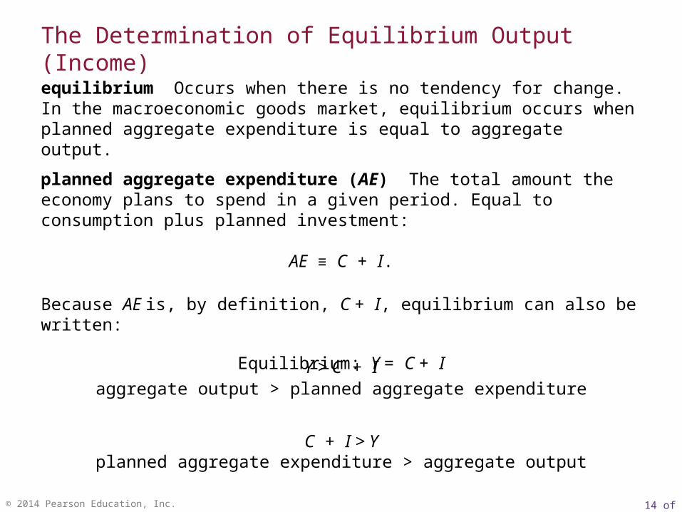
equilibrium Occurs when there is no tendency for change. In the macroeconomic goods market, equilibrium occurs when planned aggregate expenditure is equal to aggregate output.

planned aggregate expenditure (AE) The total amount the economy plans to spend in a given period. Equal to consumption plus planned investment:

AE ≡ C + I.

Because AE is, by definition, C + I, equilibrium can also be written:

Equilibrium: Y = C + I

Y > C + Iaggregate output > planned aggregate expenditure

C + I > Yplanned aggregate expenditure > aggregate output

The Determination of Equilibrium Output (Income)


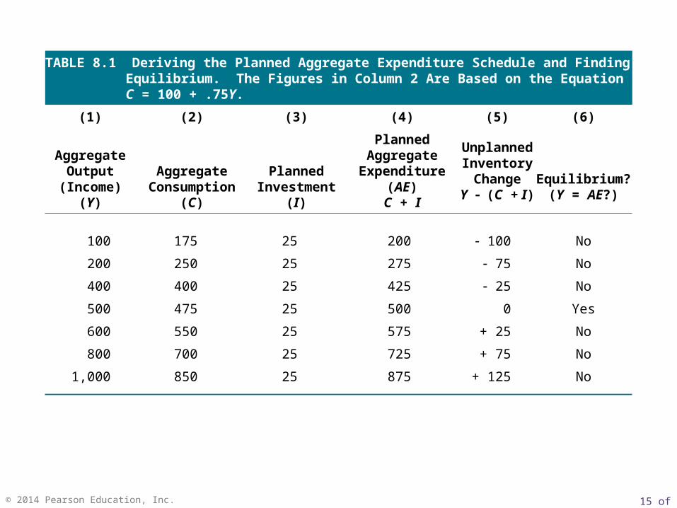
TABLE 8.1 Deriving the Planned Aggregate Expenditure Schedule and Finding Equilibrium. The Figures in Column 2 Are Based on the Equation C = 100 + .75Y.

(1) (2) (3) (4) (5) (6)

AggregateOutput

(Income) (Y)Aggregate

Consumption (C)Planned

Investment (I)

PlannedAggregate

Expenditure (AE)C + I

UnplannedInventoryChange

Y (C + I)Equilibrium?

(Y = AE?)

100 175 25 200 100 No

200 250 25 275 75 No

400 400 25 425 25 No

500 475 25 500 0 Yes

600 550 25 575 + 25 No

800 700 25 725 + 75 No

1,000 850 25 875 + 125 No


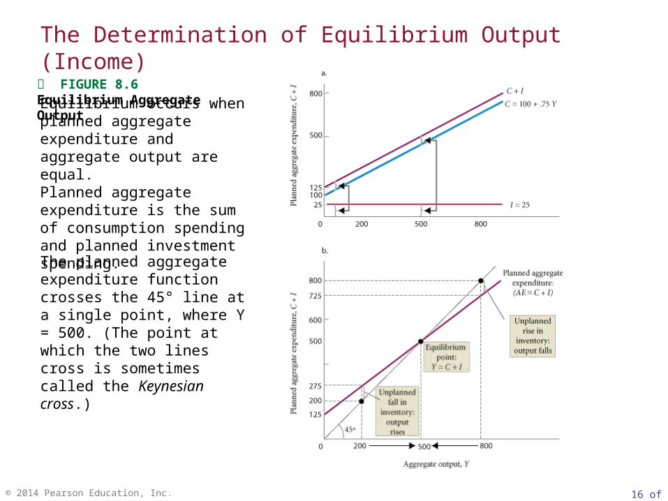
FIGURE 8.6 Equilibrium Aggregate Output

Equilibrium occurs when planned aggregate expenditure and aggregate output are equal.Planned aggregate expenditure is the sum of consumption spending and planned investment spending.

The Determination of Equilibrium Output (Income)

The planned aggregate expenditure function crosses the 45° line at a single point, where Y = 500. (The point at which the two lines cross is sometimes called the Keynesian cross.)


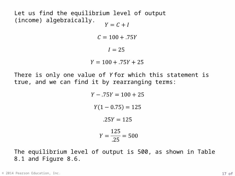
There is only one value of Y for which this statement is true, and we can find it by rearranging terms:

Let us find the equilibrium level of output (income) algebraically.

The equilibrium level of output is 500, as shown in Table 8.1 and Figure 8.6.


Because aggregate income must be saved or spent, by definition, Y ≡ C + S, which is an identity. The equilibrium condition is Y = C + I, but this is not an identity because it does not hold when we are out of equilibrium. By substituting C + S for Y in the equilibrium condition, we can write:

C + S = C + I

Because we can subtract C from both sides of this equation, we are left with:

S = I

Thus, only when planned investment equals saving will there be equilibrium.

The Saving/Investment Approach to Equilibrium

FIGURE 8.7 The S = I Approach to Equilibrium

Aggregate output is equal to planned aggregate expenditure only when saving equals planned investment (S = I).Saving and planned investment are equal at Y = 500.


The adjustment process will continue as long as output (income) is not equal to planned aggregate expenditure.

If an economy with planned spending greater than output (where unplanned inventory reductions occur) will adjust to equilibrium by increasing output, with Y going higher than before.

If planned spending is less than output, there will be unplanned increases in inventories. In this case, firms will respond by reducing output. As output falls, income falls, consumption falls, and so on, until equilibrium is restored, with Y lower than before.

As Figure 8.6 shows, at any level of output above Y = 500, such as Y = 800, output will fall until it reaches equilibrium at Y = 500, and at any level of output below Y = 500, such as Y = 200, output will rise until it reaches equilibrium at Y = 500.

Adjustment to Equilibrium


multiplier The ratio of the change in the equilibrium level of output to a change in some exogenous variable.

exogenous variable A variable that is assumed not to depend on the state of the economy—that is, it does not change when the economy changes.

The Multiplier

The size of the multiplier depends on the slope of the planned aggregate expenditure line. The steeper the slope of this line, the greater the change in output for a given change in investment.


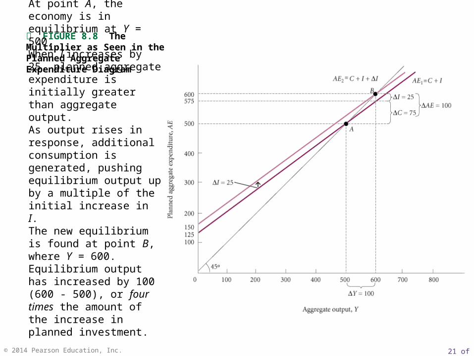
FIGURE 8.8 The Multiplier as Seen in the Planned Aggregate Expenditure Diagram

At point A, the economy is in equilibrium at Y = 500.When I increases by 25, planned aggregate expenditure is initially greater than aggregate output. As output rises in response, additional consumption is generated, pushing equilibrium output up by a multiple of the initial increase in I.The new equilibrium is found at point B, where Y = 600.Equilibrium output has increased by 100 (600 - 500), or four times the amount of the increase in planned investment.


M P SS

Y

M P SI

Y

Because S must be equal to I for equilibrium to be restored, we can substitute I for S and solve:

Therefore, Y IM P S

1

, or

Recall that the marginal propensity to save (MPS) is the fraction of a change in income that is saved. It is defined as the change in S (∆S) over the change in income (∆Y):

The Multiplier Equation

MPS

1multiplier

MPC

1

1multiplier

It follows that


An increase in planned saving from S0 to S1 causes equilibrium output to decrease from 500 to 300.

The decreased consumption that accompanies increased saving leads to a contraction of the economy and to a reduction of income.

But at the new equilibrium, saving is the same as it was at the initial equilibrium.

Increased efforts to save have caused a drop in income but no overall change in saving.

E C O N O M I C S I N P R A C T I C E

The Paradox of Thrift

An interesting paradox can arise when households attempt to increase their saving.

THINKING PRACTICALLY

1.Draw a consumption function corresponding to S0 and S1 and describe what is happening.

THINKING PRACTICALLY

1.Draw a consumption function corresponding to S0 and S1 and describe what is happening.


In this chapter, we took the first step toward understanding how the economy works.

We assumed that consumption depends on income, that planned investment is fixed, and that there is equilibrium.

We discussed how the economy might adjust back to equilibrium when it is out of equilibrium.

We also discussed the effects on equilibrium output from a change in planned investment and derived the multiplier.

In the next chapter, we retain these assumptions and add the government to the economy.

Looking Ahead


actual investment

aggregate income

aggregate output

aggregate output (income) (Y)

aggregate saving (S)

consumption function

equilibrium

exogenous variable

identity

marginal propensity to consume (MPC)

marginal propensity to save (MPS)

multiplier

planned aggregate expenditure (AE)

planned investment (I)

1. S ≡ Y − C2. 3. MPC + MPS ≡ 14. AE ≡ C + I5. Equilibrium condition: Y = AE or

Y = C + I6. Saving/investment approach to

equilibrium: S = I

7.

slope of consumption function C

MPCY

- MPCMPS 1

1

1 Multiplier

R E V I E W T E R M S A N D C O N C E P T S


CHAPTER 8 APPENDIX

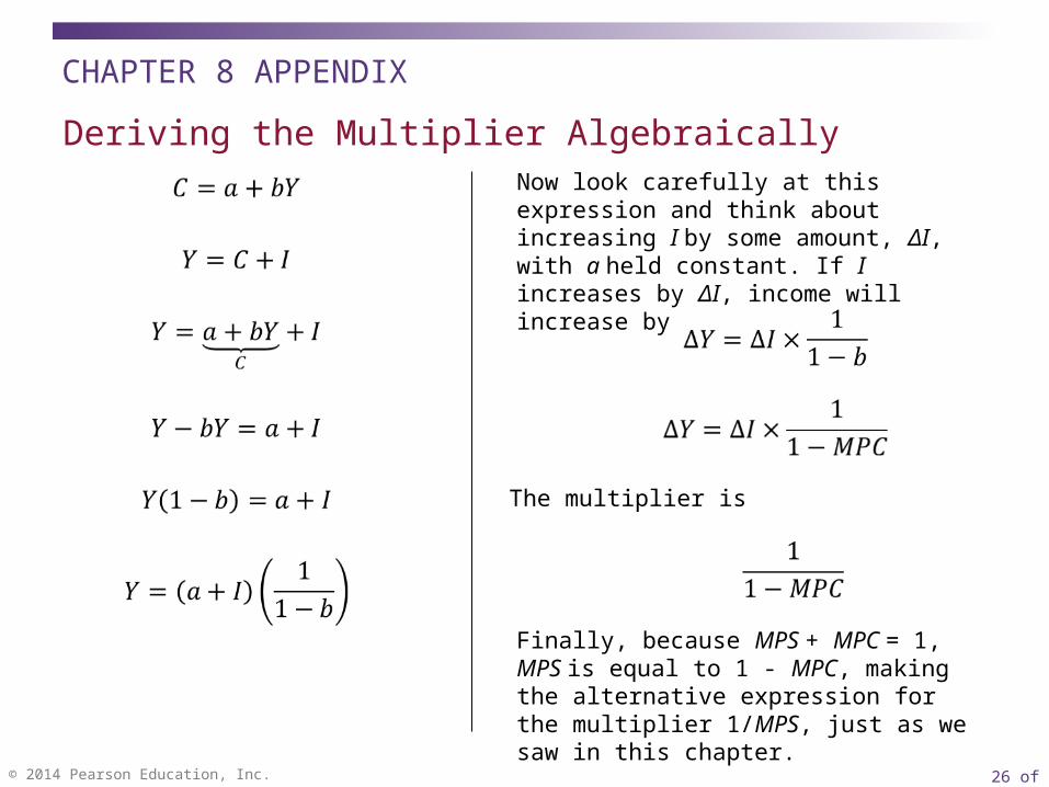
Deriving the Multiplier AlgebraicallyNow look carefully at this expression and think about increasing I by some amount, ΔI, with a held constant. If I increases by ΔI, income will increase by

The multiplier is

Finally, because MPS + MPC = 1, MPS is equal to 1 - MPC, making the alternative expression for the multiplier 1/MPS, just as we saw in this chapter.

Documents

1 of 33 © 2014 Pearson Education, Inc. CHAPTER OUTLINE 8 Aggregate Expenditure and Equilibrium Output The Keynesian Theory of Consumption Other Determinants