Embed Size (px)
Citation preview

Lo
ok In
side G
et A
ccess
Fin
d o
ut h
ow
to a
ccess p
revie
w-o
nly
con
ten
t
Ara
bia
n Jo
urn
al fo
r Scie
nce a
nd E
ngin
eerin
g
June 2
012
, Volu
me 3
7, Issu
e 4
, pp 1
101-1
110
Fin
ite Differen
ce and C
ubic In
terpolated
Pro
file Lattice B
oltzm
ann
Meth
od fo
r Pred
iction o
f Tw
o-D
imen
sional L
id-D
riven
Shallo
w C
avity
Flo
w
Abstract
In th
is pap
er, tw
o-d
imensio
nal lid
-driv
en c
avity
flow
phenom
ena a
t steady sta
te w
ere
simula
ted u
sing tw
o d
iffere
nt
scale
s of n
um
eric
al m
eth
od: th
e fin
ite d
iffere
nce so
lutio
n to
the N
avie
r–Sto
kes e
quatio
n a
nd th
e c
ubic
inte
rpo
late
d
pse
ud
o-p
artic
le la
ttice B
oltzm
ann m
eth
od. T
he a
spect ra
tio o
f cavity
was se
t at 1
, 2/3
, 1/2
and 1
/3 a
nd th
e R
ey
no
lds
nu
mber o
f 100
, 40
0 a
nd 1
,000 fo
r every
simula
tion c
onditio
n. T
he re
sults w
ere
pre
sente
d in
term
s of th
e lo
catio
n o
f
the c
en
ter o
f main
vorte
x, th
e stre
am
line p
lots a
nd th
e v
elo
city
pro
files a
t vertic
al a
nd h
orizo
nta
l mid
sectio
ns. In
this
study, it is fo
un
d th
at a
t the sim
ula
tion o
f Reynold
s num
bers 1
00 a
nd 4
00, b
oth
meth
ods d
em
onstra
te a
good
agre
em
ent w
ith e
ach o
ther; h
ow
ever, sm
all d
iscre
pancie
s appeare
d fo
r the sim
ula
tion a
t the R
eynold
s num
ber o
f
1,0
00. W
e a
lso fo
und th
at th
e n
um
ber, size
and fo
rmatio
n o
f vortic
es stro
ngly
depend o
n th
e R
eynold
s num
ber. T
he
effe
ct o
f the a
spect ra
tio o
n th
e flu
id flo
w b
ehavio
r is also
pre
sente
d.
Finite
Diffe
renc
e and
Cub
ic Inte
rpola
ted P
rofile
Lattice
Boltzm
ann M
et...
http://link
.spring
er.com
/conten
t/pd
f/10
.100
7/s1
33
69-0
12-0
22
2-5
1 o
f 32
1/1
/201
3 6
:32
PM

Related
Con
tent
Referen
ces (25)
Abou
t this A
rticle
Title
Fin
ite D
iffere
nce a
nd C
ubic
Inte
rpola
ted P
rofile
Lattic
e B
oltzm
ann M
eth
od fo
r Pre
dic
tion o
f
Tw
o-D
imensio
nal L
id-D
riven S
hallo
w C
avity
Flo
w
Jou
rnalA
rab
ian Jo
urn
al fo
r Scie
nce a
nd E
ngin
eerin
g
Vo
lum
e 3
7, Issu
e 4
, pp 1
101-1
110
Co
ver D
ate
20
12
-06-0
1
DO
I
10
.10
07/s1
3369-0
12-0
222-5
Prin
t ISS
N
13
19
-8025
On
line IS
SN
21
91
-4281
Pu
blish
er
Sp
ringer-V
erla
g
Ad
ditio
nal L
inks
Registe
r for Jo
urn
al U
pdate
s
Ed
itoria
l Board
Ab
out T
his Jo
urn
al
Manusc
ript S
ubm
ission
To
pic
s
En
gin
eerin
g, g
enera
l
Scie
nce, g
enera
l
Key
wo
rds
Fin
ite d
iffere
nce
Lattic
e B
oltzm
ann
Sh
ear c
avity
flow
Asp
ect ra
tio
Reynold
s num
ber
Au
thors
No
r Azw
adi C
he S
idik
(1)
Idris M
at S
ahat (2
)
Au
thor A
ffiliatio
ns
1. D
epartm
ent o
f Therm
oflu
id, F
aculty
of M
echanic
al E
ngin
eerin
g, U
niv
ersiti T
eknolo
gi M
ala
ysia
(UT
M), 8
1310, S
kudai, Jo
hor, M
ala
ysia
2. D
epartm
ent o
f Therm
oflu
id, F
aculty
of M
echanic
al E
ngin
eerin
g, U
niv
ersiti M
ala
ysia
Pahan
g,
Finite
Diffe
renc
e and
Cub
ic Inte
rpola
ted P
rofile
Lattice
Boltzm
ann M
et...
http://link
.spring
er.com
/conten
t/pd
f/10
.100
7/s1
33
69-0
12-0
22
2-5
2 o
f 32
1/1
/201
3 6
:32
PM

FINITE DIFFERENCE AND CUBIC INTERPOLATED PROFILE LATTICE BOLTZMANN METHOD FOR
PREDICTION OF TWO DIMENSIONAL LID-DRIVEN SHALLOW CAVITY FLOW
*Nor Azwadi Che Sidik
Senior lecturer, Department of Thermofluid
Faculty of Mechanical Engineering
Universiti Teknologi Malaysia
81310 UTM Skudai Johor
Malaysia
E-mail: [email protected]
Tel: +607-5534718; Fax:+607-5566159
Idris Mat Sahat
Lecturer, Department of Thermofluid
Faculty of Mechanical Engineering
Universiti Malaysia Pahang
26300 Kuantan Pahang
Malaysia
E-mail: [email protected]
Tel: +609-5492242; Fax:+609-6592244
*Corresponding author
FINITE DIFFERENT AND CUBIC INTERPOLATED PROFILE LATTICE BOLTZMANN METHOD FOR
PREDICTION OF TWO DIMENSIONAL LID-DRIVEN SHALLOW CAVITY FLOW
*Nor Azwadi Che Sidik
Senior lecturer, Department of Thermofluid
Faculty of Mechanical Engineering
Universiti Teknologi Malaysia
81310 UTM Skudai Johor
Malaysia
E-mail: [email protected]
Tel: +607-5534718; Fax:+607-5566159
Idris Mat Sahat
Lecturer, Department of Thermofluid
Faculty of Mechanical Engineering
Universiti Malaysia Pahang
26300 Kuantan Pahang
Malaysia
E-mail: [email protected]
Tel: +609-5492242; Fax:+609-6592244
ABSTRACT
In this paper, two-dimensional lid-driven cavity flow phenomena at steady state were simulated using two different scales of
numerical method; the finite difference solution to the Navier-Stokes equation (FDNSE) and the cubic interpolated pseudo-
particle lattice Boltzmann method (CIPLBM). The aspect ratio of cavity was set at 1, 2/3, 1/2 and 1/3 and the Reynolds
number of 100, 400 and 1000 for every simulation condition. The results were presented in terms of the location of the
center of main vortex, the streamline plots and the velocity profiles at vertical and horizontal midsection. In this study, it is
found that at the simulation of Reynolds numbers 100 and 400, both methods demonstrate a good agreement with each other,
however, small discrepancies appeared for the simulation at the Reynolds number of 1000. We also found that the number,
size and formation of vortices strongly depend on the Reynolds number. The effect of the aspect ratio on the fluid flow
behavior is also presented.
Keywords: Finite Difference; Lattice Boltzmann; Shear Cavity Flow; Aspect Ratio; Reynolds Number
1.0 INTRODUCTION
Lid-driven cavity flow is a well-known fluid flow problem where the fluid is set into motion by a part of containing
boundary. This type of flow has been used as a benchmark problem for many numerical methods due to its simple geometry
and complicated flow behaviour. However, analytical solution to this flow problem has not been confirmed to the present
day [1].
Ghia et. al [2] gives a comprehensive review on the numerical studies related to this type of fluid flows. Besides
investigating the physics of the flow, most of the papers related to the analysis of the lid-driven cavity flow aimed to validate
their newly developed numerical method. Some of them are Barragy and Carey [3] who tested their modified finite element
scheme. Other methods such finite volume by Albensoeder et. al [4], Galerkin spectral method by Auteri and Quartapelle
[5], spectral method by Auteri et. al [6], high order finite difference method by Tafti [7], simple bifurcations method by
Poliashenko and Aidun [8], lattice Boltzmann method by Guo et. al [9] and Zou et. al [10], Chebyshev projection schemes
by Botella [11], etc.
There have been some works devoted to the issue of three-dimensional effect in the cavity. An example is the work of
Chiang et. al [12] where the behaviour of end wall corner vortices is investigated numerically. Migeon et. al [13] conducted
several experiments to study the effect of the shape of the cavity and obtained good agreement when compared with
numerically predicted results.
Comparatively, little works have been conducted to investigate to transient phenomenon of the fluid flow in the cavity.
The most comprehensive work was conducted by Peng et. al [14] where they combined the seventh order upwind biased in
the advection equation and six order accuracy central finite difference of the diffusion term to obtain detailed structure of the
vortices in the system. Other researchers such as Cheng and Hung [15] recently study the effect of the aspect ratio on the
flow behaviour and Azwadi and Tanahashi [16] include the temperature effect to investigate the distribution of velocity and
temperature fields in the system.
In this study, detailed numerical investigations of lid-driven flow in a square cavity is performed with the absence of heat
transfer or heat generation in the system. The aspect ratio, AR, defined as the ratio of the height to the width of the cavity, is
varied at 1, 2/3, 1/2 and 1/3. Two different scales of numerical approaches were utilized to carry out the numerical
simulations which are the finite difference solution to the Navier-Stokes equation (macroscale) and the lattice Boltzmann
numerical method (mesoscale). In this paper, the efficiency of the later scheme is upgraded and third order numerical
accuracy is proposed from the interpolation between two mesh points. The details of the propose method will be discussed in
the next Section.
The rest of this paper is consisted of three sections. The physical domain of interest and its mathematical formulation are
described in the next section. The computational methodology and procedure are then presented, which are followed by a
detailed presentation and discussion of the numerical results. Some concluding remarks are finally drawn based on the
foregoing analysis
2. PROBLEM PHYSICS AND NUMERICAL SCHEMES
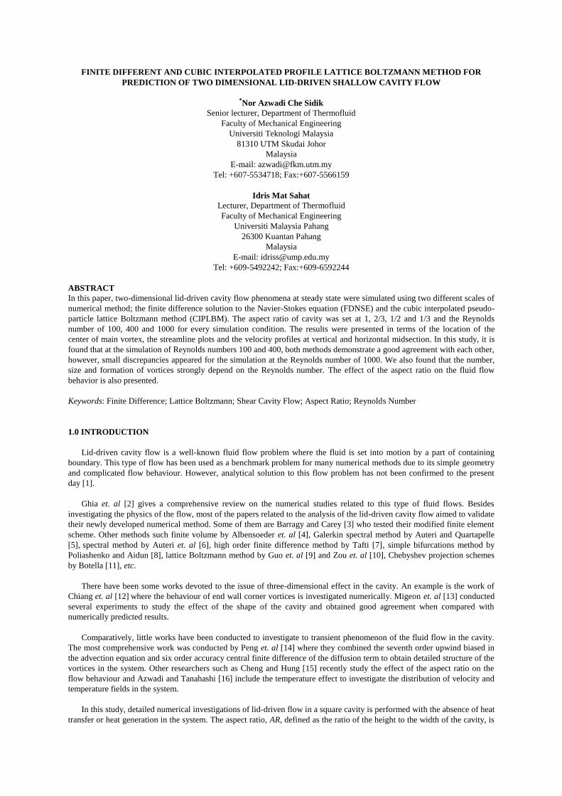
The physical model for the cavity is represented in Figure 1. The fluid in the cavity is considered as incompressible and
Newtonian fluid. The boundary condition is set as no slip wall except for the top surface.
Figure 1. Physical model of lid-driven cavity flow
In present study, two different scales of numerical approach are applied to simulate the case study in hand. They are the
well-known conventional finite different solution to the Navier-Stokes equation and the lattice Boltzmann method (LBM)
[17]. In order to obtain better accuracy of later scheme, the advection term in the governing equation of LBM is solved using
the so-called cubic interpolated pseudo-particle method proposed Yabe et. al [18]. The next section will discuss the
characteristics and their mathematical formulations of these two methods.
2.1 Finite Difference Method
The flow in the system is considered as steady, laminar and incompressible. Therefore, the flow is governed by two main
hydrodynamics equations which are the continuity equation
u
xv
y 0 (1)
and the momentum equation in x- and y-directions
uu
x v
u
y
1
p
x
2u
x2 2u
y2
(2)
uv
x v
v
y
1
p
y
2v
x2 2v
y2
(3)
In current study, the governing equations of (1), (2) and (3) are transformed into the stream function and vorticity
representation. To see this, we first bring the vorticity equation given as
v
xu
y (4)
Next, the pressure terms are eliminated by subtracting the x-derivative of (3) from the y-derivative of (2). This gives

u 2v
x2 2u
xy
v
2v
yx 2u
y2
v
x
u
xv
y
u
y
u
xv
y
3v
x3 3u
x2y
3v
y2x 3u
y3
(5)
Using the definition of vorticity defined in (4) and continuity equation defined in (1), (5) can be rewritten as follow
u
x v
y
2
x2 2
y2
(6)
The flow velocity components of u and v are then represented by the stream function equation as follow
u
y, v
x (7)
As a result, (6) can be transformed into
y
x
x
y
2
x2 2
y2
(8)
The vorticity equation in terms of the stream function is represented as follow
2
x2 2
y2 (9)
Before considering the numerical solution to the above set of equations, it is convenient to rewrite the equations in terms
of dimensionless variables. The following dimensionless variables will be used here:
Re (10)
W 2
Re (11)
X x
W,Y
y
W (12)
where Reynolds number is defined as
ReUW
In terms of these variables, (8) and (9) become
Y
X
X
Y
1
Re
2
X 2 2
Y 2
(13)
2
X 2 2
Y 2 (14)
In order to solve (13) and (14) using digital computer, the so-called finite difference method is applied with second order
accuracy and can be expressed as follow
i, j
i1, j i1, j
X2
i, j1 i, j1
Y2
Rei, j1 i, j1 i1, j i1, j
4XYRe
i1, j i1, j i, j1 i, j1 4XY
2
X 2
2
Y 2
(15)
Treatment at the boundaries can be done as follow

1, j 22, j
X 2 (17)
imax , j 2imax1, j
X 2 (18)
i,1 2i,2
X 2 (19)
i, jmax 2i, jmax1 U Y
Y 2
(20)
Note that, imax and jmax are the maximum grid point in x-and y-direction.
Weinan and Liu [19] conducted numerical investigation on the stability of vorticity boundary nodes by using the finite
difference scheme. We found that the scheme produced unstable results if the unsteady term is included in the discretization
procedure. However, in the present analysis, the stability of the vorticity boundary nodes is not our major concern since the
unsteady term in our formulation is neglected.
In order to obtain an accurate result in every simulation condition, the convergence criteria were set up as follow
present previous and presentprevious 1012
(21)
2.2 Cubic Interpolated Profile Lattice Boltzmann Method
Lattice Boltzmann Method (LBM) is a recent alternative mesoscale method to simulate fluid flow problems. LBM
evolves from the lattice gas automata method, predict the phenomena of fluid flow by reconstructing the translation and
collision processes of the particles [20]. The lattice Boltzmann equation with BGK collision function [21] is written as
follow
ft
c,xfx
c,yfy
1
feq f (22)
where
f is the density distribution function and
feq
is the Boltzmann-Maxwell equilibrium distribution functions defined
as
feq
1
2RT
D
2exp
cu
2RT
2
1c u
RTc u
2
2 RT 2u
2
2RT
(23)
Figure 2. The BGK approximation for D2Q9 lattice model
The
feq
is chosen in a way such that it satisfies the hydrodynamics behavior of the problem. For two-dimension and
nine-lattice velocity model (D2Q9), the
feq
can be written as
feq 13c u 4.5
21.5u
2 (24)
6
2
3
4
5
7
8 9
1

where
1 4 9 ,
2,3,4,5 1 9 and
6,7,8,9 1 36. The lattice velocity for D2Q9 is defined as
c
0,0 ,
1,0 , 0,1 ,
1,1 ,
1
2,3,4,5
6,7,8,9
(25)
and the lattice model is shown in Figure 2.
The kinematic viscosity for this model is related to the time relaxation as
3. In CIPLBM scheme, the profile
between the two nodes is interpolated using third order polynomial as follow
F, i, j a1X a2Y a3 X a4Y fx X a5Y a6X a7 Y a4Y fy Y fx (26)
where
a12d fx, i1, j fx, i, j X
X 3 (27)
a2a8 dx, jX
X 2Y (28)
a33d fx, i1, j fx, i, j X
X 2 (29)
a4 a8dx, jX dy, jY
XY (30)
a52d j fy, i, j1 Y
Y 3 (31)
a6a8 dy, jY
XY 2 (32)
a73d j fy, i, j1 2 fy, i, j Y
Y 2 (33)
a8 f, i, j f, i1, j f, i, j1 f, i1, j1 (34)
where
di f, i, j f, i1, j and
d j f, i, j f, i, j1.
The spatial derivatives of (26) are given by
Fx,i, j 3a1X 2a2Y a3 a4 a6Y Y fx,i, j (35)
Fy,i, j a2X a4 X 3a5Y 2a6X 2a7 Y fy,i, j (36)
In two-dimensional case, the advected profile is approximated as follow
f, i, jn*
F, i, j x x , y y (37)
fx,i, jn*
Fx,i, j x x , y y (38)
fy,i, jn*
Fy,i, j x x , y y (39)
where
x cx,it and
y cy,it .

3. RESULTS AND DISCUSSION
3.1 Simulation Results for Aspect Ratio = 1.0
The simulation results computed from FDNSE and CIPLBM were firstly compared with the benchmark solution of two-
dimension lid driven cavity flow provided by Ghia et. al [2]. This type of fluid flow is chosen as our test case due to its rich
vortex structures, simple geometry and related to many engineering applications such as heat exchangers, solar power
collectors, biomedical, etc. Table 1 shows the computed position of centre of main vortex for the case in hand using 100 x
100 mesh size for both approaches. As can be seen from the table, FDNSE gives slightly higher values of error compared to
CIPLBM when both compared to Ghia’s solutions. This expected error is due to lower mesh resolution as compared to those
applied by Ghia et. al. However, the results are still acceptable and the errors are kept below 3% and can be accepted in real
engineering application.
Table 1. Center of primary vortex for aspect ratio 1.0
Re Center Ghia et. al [2] FD-NSE Error (%) CIP-LBM Error (%)
100 X 0.6172 0.63 2.07 0.63 2.07
Y 0.7344 0.75 2.12 0.75 2.12
400 X 0.5547 0.57 2.76 0.56 0.96
Y 0.6055 0.62 2.39 0.6 0.91
1000 X 0.5313 0.54 1.64 0.53 0.24
Y 0.5625 0.58 3.11 0.56 0.44
3.2 Simulation Results for Aspect Ratio 2/3, 1/2 and 1/3.
Figure 3 shows plots of streamline in the cavity at aspect ratio 2/3 when the system achieved steady state. The centre of
vortex shifted form one-third of the cavity height measured from the top wall at low Reynolds number to the centre of cavity
at Re = 1000. These plotted results clearly demonstrate a good agreement between these two simulation approaches.
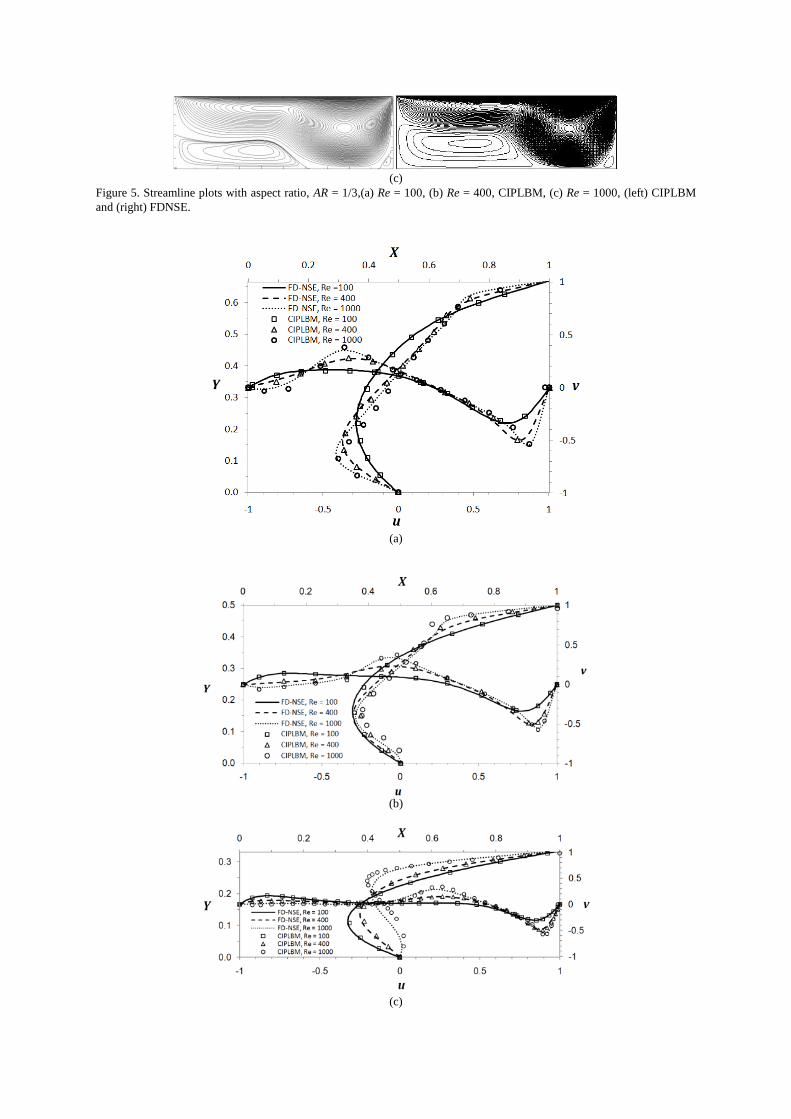
For the simulation at aspect ratio, AR = 1/2 and 1/3, as can be seen from Figures 4 and 5, both methods yields
outstanding agreement when the generated centre of primary and secondary vortices in the cavity is compared. However,
CIPLBM failed to reproduce the secondary vortices for Re = 100 due to low mesh resolution.
For the simulation at low Reynolds number, the primary vortex appears at the center height of the cavity and near to the
right wall. Two equal sizes of vortices are formed near the bottom left and right corner of the cavity. As the Reynolds
number is increased, the left corner vortex grows faster than the right corner vortex. The growth of the right corner vortex is
retarded due to the formation of main vortex and compresses this corner vortex. All of these findings are in agreement with
previous researchers [22-25]
(a)
(b)

(c)
Figure 3. Streamline plots with aspect ratio, AR = 2/3,(a) Re = 100, (b) Re = 400, CIPLBM, (c) Re = 1000, (left) CIPLBM
and (right) FDNSE.
3.3 Velocity Profile at Horizontal and Vertical Midsection.
Figure 6 shows the plot of horizontal and vertical component of velocity profiles of at mid-width and mid-height of the
cavity for all aspect ratios. In this figure, X and Y represent width and height of the cavity while u and v represent the
horizontal and vertical components of flow velocity respectively. It can be seen that the macroscale approach of FDNSE is in
good agreement with mesoscale of CIPLBM when the computed velocity profiles are compared. Small difference can only
be seen for the computations at high Reynolds number. Validation with experimental data will be carried out in near future
research to investigate the accuracy of these two approaches for the simulation at high Reynolds numbers.
(a)
(b)
(c)
Figure 4. Streamline plots with aspect ratio, AR = 1/2,(a) Re = 100, (b) Re = 400, CIPLBM, (c) Re = 1000, (left) CIPLBM
and (right) FDNSE.
(a)
(b)
(c)
Figure 5. Streamline plots with aspect ratio, AR = 1/3,(a) Re = 100, (b) Re = 400, CIPLBM, (c) Re = 1000, (left) CIPLBM
and (right) FDNSE.
(a)
(b)
(c)

Figure 6. Comparisons of horizontal and vertical velocity components for aspect ratio (a) AR = 2/3, (b) AR = 1/2 and (c) AR
= 1/3.
4. CONCLUSSION
In this paper, the fluid flow driven by shear force has been simulated in rectangular cavities using macro and meso-scale
approaches. In macroscale approach, the Navier-Stokes equations were transformed into vorticity and stream function
formulation in order to reduce the dependent parameters in the system. Then the conventional second order central
difference was used for discretisation process and all of these difference equations were translated into FORTRAN computer
language. For the computation at mesoscale approach, the conventional lattice Boltzmann approach was combined with the
cubic interpolated profile method to improve the spatial accuracy of the scheme. The case study of shallow lid-driven cavity
flow was simulated using these two different scales of numerical methods. From the comparison of the plotted streamlines
and velocity profiles in the system, we can say that both methods are in excellent agreement and their capability in solving
fluid flows phenomena is proven. The effect boundary condition in the lateral direction (three-dimensional case) will be
considered in our near future investigations.
REFERENCES
[1] F. Pan and A. Acrivos, “Steady Flow in Rectangular Cavities”, J. Fluid Mech., 28(1967), pp. 643-655.
[2] U. Ghia, K. N. Ghia and C. T. Shin, “High-Re Solutions for Incompressible Flow using the Navier–Stokes Equations and
a Multigrid Method”, J. Comp. Phys., 48(1982), pp. 367-411.
[3] E. Barragy and F.C. Carey, “Stream Function-Vorticity Driven Cavity Solution using Finite Elements”, Comp & Fluids,
26(1997), pp. 453-468.
[4] S. Albensoeder, H.C. Kuhlmann and H.J. Rath, “Multiplicity of Steady Two-Dimensional Flows in Two-Sided Lid-
Driven Cavities”, Theoretical Comp. Fluid Dynamics, 14(2001), pp. 223–241.
[5] F. Auteri and L. Quartapelle, “Galerkin Spectral Method for the Vorticity and Stream Function Equations”, J. Comp.
Phys., 149(1999), pp. 306–332.
[6] F. Auteri, L. Quartapelle and L. Vigevano, “Accurate Omega-Psi Spectral Solution of the Singular Driven Cavity
Problem”, J. Comp. Phys., 180(2002), pp. 597-615.
[7] D. Tafti, “Comparison of Some Upwind-Biased High-Order Formulations with a Second-Order Central-Difference
Scheme for Time Integration of the Incompressible Navier–Stokes Equations”, Comp. & Fluids, 25(1996), pp. 647-665.
[8] M Poliashenko and C.K. Aidun, “A Direct Method for Computation of Simple Bifurcations”, J. Comp. Phys., 120(1995),
pp. 246-260.
[9] Z. Guo, B. Shi and N. Wang, “Lattice BGK Model for Incompressible Navier–Stokes Equation”, J. Comp. Phys.,
165(2000), pp. 288–306.
[10] S. Huo and Q. Zuo, “Simulation of Cavity Flow by Lattice Boltzmann Method”, J. Comp. Phys., 118(1995), pp. 329-
347.
[11] O. Botella, “On the Solution of the Navier-Stokes Equations using Chebyshev Projection Schemes with Third-Order
Accuracy in Time”, Comp. & Fluids, 26(1997), pp. 107-116.
[12] T.P. Chiang, R.R. Hwang and W.H. Sheu, “On End-Wall Corner Vortices in a Lid-Driven Cavity”, J. Fluids Eng.,
119(1997), pp. 201-204.
[13] C. Migeon, A. Texier and G. Pineau, “Effect of Lid-Driven Cavity Shape on the Flow Establishment”, J. Fluids and
Structures, 14(2000), pp. 469-488.
[14] Y.F. Peng, Y.H. Shiau and R.R. Hwang, “Transition in a 2-D Lid-Driven Cavity Flow”, Comp. & Fluid, 32(2003), pp.
337-352.
[15] M. Cheng and K.C. Hung, “Vortex Structure of Steady Flow in a Rectangular Cavity”, Comp. & Fluids, 35(2006), pp.
1046-1062.
[16] C. S. Nor Azwadi and T. Tanahashi, “Simplified Thermal Lattice Boltzmann in Incompressible Limit”, Intl. J. Modern
Phys. B, 20(2006), pp. 2437-2449.

[17] C. S. Nor Azwadi and T. Tanahashi, “Simplified Finite Difference Thermal Lattice Boltzmann Method”, Intl. J. Modern
Phys., 22(2008), pp. 3865-3876.
[18] H. Takewaki, A. Nishigushi and T. Yabe, “Cubic Interpolated Pseudo-particle Method (CIP) for Solving Hyperbolic
Type Equations”, J. Comp. Phys., 61(1985), pp. 261-268.
[19] E. Weinan and J.G. Liu, “Vorticity Boundary Condition and Related Issues for Finite Difference Schemes”, J. Comp.
Phys., 124(1996), pp. 368–382.
[20] C. S. Nor Azwadi and T. Tanahashi, “Three-Dimensional Thermal Lattice Boltzmann Simulation of Natural Convection
in a Cubic Cavity”, Intl. J. Modern Phys. B, 21(2007), pp. 87-96.
[21] P. L. Bhatnagar, E. P. Gross and M. Krook, “A Model for Collision Process in Gasses 1, Small Amplitude Process in
Charged and Neutral One Component System”, Phys. Rev., 70(1954), pp. 511-525.
[22] L. Wang, Z. Guo and C. Zheng, “Multi-Relaxation-Time Lattice Boltzmann Model for Axisymmetric Flows”, Comp. &
Fluids, 39(2010), pp. 1542-1548
[23] T. Zhang, B. Shi and Z. Chai, “Lattice Boltzmann Simulation of Lid-Driven Flow in Trapezoidal Cavities”, Computers
and Fluids, 39(2010), pp. 1977-1989.
[24] C. F. Ho, C. Chang, K. H. Lin and C. A. Lin, “Consistent Boundary Conditions for 2D and 3D lattice Boltzmann
Simulations”, Comp. Mod. Eng. Science, 44(2009), pp. 137-155
[25] A. A. Mohamad, M. El-Ganaoui and R. Bennacer, “Lattice Boltzmann Simulation of Natural Convection in an open
ended cavity”, Intl. J. Thermal Sciences, 48(2009), pp. 1870-1875.