1 Multipath Parameter Estimation from OFDM Signals in ... · PDF file1 Multipath Parameter Estimation from OFDM Signals in Mobile Channels Nick Letzepis, Member, IEEE, Alex Grant,

1

Multipath Parameter Estimation from OFDM

Signals in Mobile Channels

Nick Letzepis, Member, IEEE, Alex Grant, Senior Member, IEEE,

Paul Alexander Member, IEEE, David Haley, Member, IEEE

Abstract

We study multipath parameter estimation from orthogonal frequency division multiplex signals

transmitted over doubly dispersive mobile radio channels. We are interested in cases where the trans-

mission is long enough to suffer time selectivity, but short enough such that the time variation can be

accurately modeled as depending only on per-tap linear phase variations due to Doppler effects. We

therefore concentrate on the estimation of the complex gain, delay and Doppler offset of each tap of

the multipath channel impulse response. We show that the frequency domain channel coefficients for

an entire packet can be expressed as the superimposition of two-dimensional complex sinusoids. The

maximum likelihood estimate requires solution of a multidimensional non-linear least squares problem,

which is computationally infeasible in practice. We therefore propose a low complexity suboptimal

solution based on iterative successive and parallel cancellation. First, initial delay/Doppler estimates

are obtained via successive cancellation. These estimates are then refined using an iterative parallel

cancellation procedure. We demonstrate via Monte Carlo simulations that the root mean squared error

statistics of our estimator are very close to the Cramer-Rao lower bound of a single two-dimensional

sinusoid in Gaussian noise.

I. INTRODUCTION

In wireless communications, reflection and diffraction of the transmitted radio signal results in

the superimposition of multiple complex-scaled and delayed copies of the signal at the receiver.

N. Letzepis and A. Grant are with the Institute for Telecommunications Research, University of South Australia, e-mail:

[email protected], [email protected]. P. Alexander and D. Haley are with Cohda Wireless Pty.

Ltd., e-mail: paul.alexander,[email protected].

This work was supported by Cohda Wireless Pty. Ltd. and the Australian Research Council under grant LP0775036.

November 16, 2010 DRAFT

arX

iv:1

011.

2809

v2 [

cs.I

T]

15

Nov

201

0

2

This type of channel is commonly referred to as a multipath channel. In some instances, the

multiple copies add constructively, and in others destructively resulting in multipath fading.

When the coherence bandwidth of the channel is smaller than the bandwidth of the radio signal

then the fading is termed frequency selective [1]. We assume the reader is familiar with standard

wide-sense stationary uncorrelated scattering models, for an overview see e.g. [2].

Orthogonal frequency division multiplexing (OFDM) is a transmission strategy specifically

designed to combat frequency selective channels with relatively low receiver complexity [3–

5]. In OFDM, the signal bandwidth is divided into several non-overlapping (hence orthogonal)

narrowband subcarriers where the width of each subchannel is chosen such that it is approxi-

mately frequency non-selective. Thus only a single tap equaliser per subchannel is required to

compensate for the multipath fading. Together with the use of the fast Fourier transform (FFT),

this results in a low complexity way to handle frequency-selective channels. As such, OFDM is

now the basis of many current and emerging wireless communications standards, see [6, 7] for an

overview. Many of these standards are targeted for outdoor mobile applications, e.g. 802.11p [8].

Mobility causes the multipath channel (and hence frequency selectivity) to change with time. If

the mobility is fast enough compared to the symbol rate, then the channel impulse response may

vary significantly within an OFDM packet. Extensive field trials have shown that this is indeed the

case for the transmission of 802.11 OFDM signals in vehicular environments [9]. Time-varying

multipath channels such as these are commonly termed doubly-dispersive [10–12].

In general, a realization of a doubly selective multipath channel time-varying impulse response

can be modeled in continuous time as

c(t, τ) =P∑p=1

ap(t)δ(τ − τp)

where c(t, τ) is the response at delay τ to an impulse at time t, where δ(τ) denotes the Dirac-delta

function. The ap(t) are the time-varying complex amplitude (magnitude and phase) of tap p, with

delay τp. The number of resolvable multipath components is P . The ap(t) may aggregate many

more unresolvable multipath components, typically resulting in Ricean or Rayleigh statistics for

these parameters.

Note that for sufficiently short time durations, mobility-induced Doppler shifts manifest as

linear variations of the phase of ap(t) with time. In this paper, we consider the special case


3

where the OFDM packet duration is short enough such that we can model the channel as

c(t, τ) =P∑p=1

ape−j2πνptδ(τ − τp), (1)

where ap, τp and νp respectively denote the complex gain, delay and Doppler frequency (relative

to the nominal carrier frequency) of tap p. These parameters are all assumed to be constant

over the duration of an OFDM packet. In a physical sense, this implies that changes in the

relative distance and velocity between the transmitter, receiver and scatterers are negligible over

the duration of an OFDM packet. This model is consistent with the geometric-stochastic model

presented in [13] for short observation windows, and has been validated experimentally in [9].

In this paper, we concentrate on joint estimation of ap, τp and νp of the multipath components

assuming perfect knowledge of the transmitted OFDM symbols. This is a practical assumption,

e.g. a transmitted training/pilot signal, or the receiver is able to decode the signal without error

(via a forward error correction code). Estimation of these parameters is useful in a number

of areas: channel sounding and characterisation; channel prediction; reducing channel state

information for feedback in adaptive communications; and radar. Estimation of these parameters

in the OFDM setting has been studied previously by a number of researchers from both the

communications and radar fields. Channel estimation via an approximate maximum likelihood

parameter search algorithm was proposed by Thomas et al. [14]. Their iterative algorithm was

based on an approximation of the maximum likelihood function, where the multipath gain

values are substituted with their least-squares estimates. In the radar community, estimation

of delay/Doppler is vital for determination of target range and velocity. Berger et al. [15]

studied the problem of extracting the target range/velocity information from the OFDM signal

in a passive multi-static radar system [16] using digital audio/video broadcasted signals as

illuminators of opportunity. They set up the problem as a sparse estimation problem to use

recent results from compressed sensing [17]. In particular, they employ the orthogonal matching

pursuit algorithm [18, 19], which is in an iterative algorithm that successively removes previously

estimated multipath components from the received signal to estimate new components. Note that

Taubock et al. [20, 21] also consider compressed sensing to estimate the OFDM channel coeffi-

cients. However, their interest is not in the estimation of delays/Doppler, but in the frequency/time

channel coefficients.

In this paper we begin with a continuous-time model of the transmitted OFDM signal and


4

derive the received matched filtered signal from first principles. Assuming the delay-spread of the

channel does not exceed the cyclic-prefix and the pass-band of the receive/transmit filters exceed

the signal bandwidth (with negligible pass-band ripple), we show that the resulting frequency

domain channel coefficients can be represented as the superimposition of two-dimensional (2-

D) complex sinusoids, where each 2-D frequency is proportional to the delay and Doppler of

each multipath component. Similar observations have been made by Wong and Evans [22, 23]

although without detailed justification. Under a similar setting they consider estimation using

only OFDM pilot symbols and propose channel prediction algorithms based on the estimation

of channel parameters via a rotational invariance technique. Using this method, they reformulate

the problem as a one-dimensional estimation problem.

Parameter estimation of 2-D sinusoids in a general setting has been studied extensively many

years prior to the work of Wong and Evans [22, 23]. Estimation methods and the Cramer-Rao-

Lower-Bound (CRLB) for the single 2-D sinusoid case was investigated by Chien [24]. Kay

and Nekovei [25] proposed a low complexity estimator that operates on the phase of the noisy

2-D sample data. For the estimation of the superposition of multiple 2-D sinusoids: Bresler and

Macovski employ a 2-D version of Prony’s method [26]; Rao et al. [27] use a similar polynomial

rooting approach; and recently Kliger and Francos [28] consider maximum-likelihood estimation

with a maximum a-posteriori (MAP) model order selection rule for the case where the number

of sinusoids is unknown.

In this paper we concentrate purely on the estimation of the complex amplitude, delay and

Doppler of each multipath tap, assuming the number of taps is known. Our results can be

straightforwardly extended to the case where the number of taps is unknown using well-known

model-order selection methods [29]. The maximum-likelihood approach requires the solution to

a multi-dimensional nonlinear least-squares estimation problem [30] and hence has complexity

that is prohibitive in practice [26–28]. We propose a low-complexity algorithm based on a two-

stage process: first, an initial estimation; followed by a refinement proceedure. In the same

spirit as [14, 15, 28] the initial estimation algorithm is based on successive cancellation, whereby

multipath components are subtracted from the original signal after they are detected. In each

iteration, the delay/Doppler is estimated using periodogram search [24, 25] via a 2-D bisection

algorithm. The multipath complex amplitudes are then obtained via standard linear least-square

estimation [31]. Moreover, we show that this secondary problem can be written in terms of


5

the ambiguity function [32]. Once initial estimates have been obtained, we then propose an

iterative refinement algorithm based on parallel cancellation. Each iteration of the refinement

involves subtracting all multipath components from the received signal except the component

of interest, which is re-estimated using the 2-D bisection algorithm. This refinement process

yields significant improvements over the standard successive cancellation approach. We show

via Monte-Carlo simulations that this refinement algorithm achieves performance very close to

the CRLB for single 2-D sinusoid estimation.

The remainder of our paper is organised as follows. In Section II we state the system model

and derive from first principles the received match filtered frequency domain OFDM symbols. In

Section III we derive the transmit signal ambiguity function. Then in Section IV we present our

proposed estimation algorithm and enhanced refinement process. Simulation results are presented

in Section V. Finally, concluding remarks are given in Section VI.

II. SYSTEM MODEL

Consider a K subcarrier OFDM system, where packets of length L OFDM symbols are

transmitted. Let X ∈ CL×K denote a packet of complex OFDM symbols. Thus Xl,k, the l, kth

element of X , denotes the lth symbol transmitted on subcarrier k, for l = 1, . . . , L and k =

1, . . . , K. In practical OFDM systems, a certain number null subcarriers are employed to simplify

receiver design [5]. To incorporate this feature, we let K denote the set of null subcarrier indices.

Thus, Xl,k = 0 for all k ∈ K and l = 1, . . . , L. For all other subcarriers, i.e. k /∈ K, we

assume Xk,l ∈ X , where X ⊂ C is an arbitrary complex constellation. These symbols are drawn

randomly, independently and uniformly from X , which is normalised to have unit average energy.

Thus E[|Xl,k|2] = 1 for k /∈ K and E[Xl,kX∗n,m] = 0 for any n 6= l or m 6= k. The receiver

is assumed to have complete knowledge of the transmitted symbols Xl,k, e.g. a pilot/training

signal, or from the feedback of error-free decoder decisions.

Let x(t) =∑L

l=1 xl(t) denote the complex baseband continuous-time transmitted OFDM

signal, where

xl(t) =1√KL

K∑k=1

Xl,kej2π(k−1−bK/2c)(t−Tcp)/Tw(t− (l − 1)Td), (2)

is the lth OFDM symbol, Td is the OFDM symbol duration (seconds), 1/T is the subcarrier

spacing (Hz), Tcp = Td − T is the cyclic prefix duration (seconds), and w(t) is a windowing


6

function such that

w(t) =

w(t) 0 ≤ t ≤ Td

0 otherwise,(3)

and∫ Td

0|w(t)|2 dt = 1. A simple choice of windowing function is w(t) = 1/

√Td. Note that

the assumption w(t) = 0 for t /∈ (0, Td) is not necessarily required, but we assume this for

simplicity. In practice, (2) is implemented in the discrete time domain via the inverse discrete

Fourier transform (IDFT) [5].

We assume transmit and receive filter impulse responses gT(t) and gR(t) respectively, and

let g(t) ,∫∞−∞ gT(u)gR(t − u) du denote the combined transmit/receive filter response.Thus,

using (1), we write the overall channel response as

h(t, τ) =

∫ ∞−∞

g(u)c(t, τ − u) du =P∑p=1

ape−j2πνptg(τ − τp). (4)

Application of the overall channel response (4) to (2) plus additive Gaussian white noise (AWGN)

yields the received continuous-time baseband signal,

y(t) =∑l′

∫ ∞−∞

xl′(t− τ)h(t, τ) dτ + z(t), (5)

where z(t) =∫∞−∞ z(t − u)gR(u) du, and z(t) is an additive white Gaussian noise (AWGN)

process. Assuming perfect OFDM symbol synchronism, the receiver discards the cyclic prefix

and performs the matched filter to the transmitted sinusoids, i.e.

Yl,k =1√KL

∫ lTd

Tcp+(l−1)Td

y(t)w∗(t− (l − 1)Td)e−j2π(k−1−bK/2c)(t−Tcp)/T dt, (6)

for k = 1, . . . , K and l = 1, . . . , L. Note that in practice, Yl,k is obtained via the discrete Fourier

transform (DFT) [5]. We assume the pass-band of filters gT and gR exceed the signal bandwidth.

In addition, we assume maxp τp < Tcp and maxp |νp| < 1/T , so that inter-symbol interference

(ISI) and inter-carrier interference (ICI) can be considered negligible. Under these assumptions,

in Appendix I we show that the matched filtered output (6) can be written in matrix form

Y = H X +Z, (7)

where denotes the element-wise (Hadamard) product, Y ∈ CL×K is the received matrix of

filtered noisy OFDM symbols, Z ∈ CL×K is a matrix of independent identically distributed


7

(i.i.d.) zero mean complex Gaussian random variables with variance σ2, and H ∈ CL×K are the

frequency domain channel coefficients,

Hl,k =P∑p=1

ape−j2πνpTd(l−1)e−j2π(k−1−bK/2c)τp/T . (8)

In relation to (7), we define the signal-to-noise ratio (SNR) as snr , E [‖X‖2] /(Lσ2) =

(K − |K|)/σ2, where ‖ · ‖ denotes the Frobenius norm [33].

From inspection of (8), we see that it is simply the superimposition of 2-dimensional (2-D)

complex exponential signals. We may also express H as the matrix product

H = Ψ(ν)diag(a)Φ†(τ ), (9)

where diag(a) denotes a P × P diagonal matrix with diagonal entries a = (a1, . . . , aP ), and

Ψl,p(ν) = ψl(νp) , e−j2π(l−1)νpTd (10)

Φk,p(τ ) = φk(τp) , ej2π(k−1−bK/2c)τp/T , (11)

for p = 1, . . . , P , l = 1, . . . , L and k = 1, . . . , K. As we shall see later, the separation of the

parameters in this matrix form will simplify the development of our estimation algorithms.

In the analysis that is to follow, we will make use of the vectorised version of (7). Let

y = vec(Y ) = (Y1,1, . . . , YL,1, Y1,2, . . . , YL,2, . . . , Y1,K , . . . , YL,K)′, and z = vec(Z) then

y = Ω(τ ,ν,X)a+ z. (12)

where the KL× P matrix Ω is a function of τ , ν, and X as follows,

Ω(τ ,ν,X) =

X1,1ψ1(ν1)φ∗1(τ1) X1,1ψ1(ν2)φ∗1(τ2) . . . X1,1ψ1(νP )φ∗1(τP )...

......

XL,1ψL(ν1)φ∗1(τ1) XL,1ψ1(ν2)φ∗1(τ2) . . . XL,1ψL(νP )φ∗1(τP )

X1,2ψ1(ν1)φ∗2(τ1) X1,2ψ1(ν2)φ∗2(τ2) . . . X1,2ψ1(νP )φ∗2(τP )...

......

XL,2ψL(ν1)φ∗2(τ1) XL,2ψ1(ν2)φ∗2(τ2) . . . XL,2ψL(νP )φ∗2(τP )...

......

X1,Kψ1(ν1)φ∗K(τ1) X1,Kψ1(ν2)φ∗K(τ2) . . . X1,Kψ1(νP )φ∗K(τP )...

......

XL,KψL(ν1)φ∗K(τ1) XL,KψL(ν2)φ∗K(τ2) . . . XL,KψL(νP )φ∗K(τP )

, (13)

where (·)∗ denotes the complex conjugate.


8

III. AMBIGUITY FUNCTION

The ambiguity function of the transmitted signal x(t) is defined as the inner product of the

signal with a delayed, frequency shifted version of itself [32]

Ax(τ, ν) =

∫ ∞−∞

x(t)x∗(t− τ)e−j2πνt dt. (14)

In the context of OFDM communications the ambiguity function has been used often as a tool

for pulse design and optimisation [10, 11]. In radar systems, the ambiguity function plays an

important role in determining target range and velocity resolution [32]. In this section we derive

the ambiguity function of the transmitted OFDM signal and highlight important characteristics

that will affect the delay/Doppler estimation problem. Moreover, as we shall see later, parts of

the estimation problem can be written succinctly in terms of the ambiguity function. In this

direction, substitution of (2) into (14) yields the following result.

Theorem 1 (OFDM Ambiguity Function). For a general windowing function w(t), let Aw(ν, τ)

denote its ambiguity function. The ambiguity function of the OFDM signal (2) is,

Ax(τ, ν) =e−jπKτ/T

KL

∑l,k,l′,k′

Xl,kX∗l′,k′e

−j2π(k−k′)Tcp/T ej2π(k′−1)τ/T e−j2πTd(l−1)

(ν− k−k′

T

)

× Aw(τ + (l′ − l)Td, ν + (k′ − k)/T ). (15)

Due to the quadruple summation, numerical evaluation of (15) is computationally demanding.

However, under some common practical design assumptions we can make further simplifications.

Firstly, the windowing function is usually designed such that Aw(τ, ν) ≈ 0 for |τ | > Td. Window

functions of the form (3) will have this property. Thus the terms when l′ 6= l in the summation

of (15) are approximately zero. Secondly, although Aw(τ, ν) cannot be considered negligible

for |ν| > (k′ − k)/T , since Xl,k are i.i.d. with zero mean and unit variance by assumption

(except for the null subcarriers, which have zero power), the summation of terms over k 6= k′

will approach zero for large K and/or L. In addition, since we are primarily concerned with

delay and Doppler in the region 0 ≤ τ ≤ Tcp and |ν| 1/T , where there is negligible variation

in Aw(τ, ν), we may assume Aw(τ, ν) ≈ Aw(0, 0), which only introduces a constant phase

offset, since |Aw(0, 0)|2 = 1. Hence we ignore the complex scaling affects of Aw(τ, ν) and


9

approximate (15) as

Ax(τ, ν) ≈ Ax(τ, ν) ,1

KL

∑k,l

|Xl,k|2e−j2π(l−1)νTdej2π(k−1−bK/2c)τ/T . (16)

In light of (15), note that (16) is also the ambiguity function when ISI and ICI can be considered

negligible.

For phase shift keying (PSK) modulation, |Xl,k| = 1 with no null subcarriers, i.e. K = ∅, then

using the geometric summation formula, the ambiguity function (16) further simplifies to

Ax(τ, ν) ≈ e−jπKτ/T sinc(πK

τ

T

)sinc (πLνTd) , (17)

where sinc(x) = sin(x)/x. Note that (17) is also equal to the expectation of (15) over the

transmitted symbols Xl,k, i.e. it is the expected ambiguity function, E [Ax(τ, ν)], for an arbitrary

signal constellation X with zero mean and unit variance. In many OFDM standards, subcarrier

k = bK/2c+ 1 is a null subcarrier. For these special cases (17) becomes,

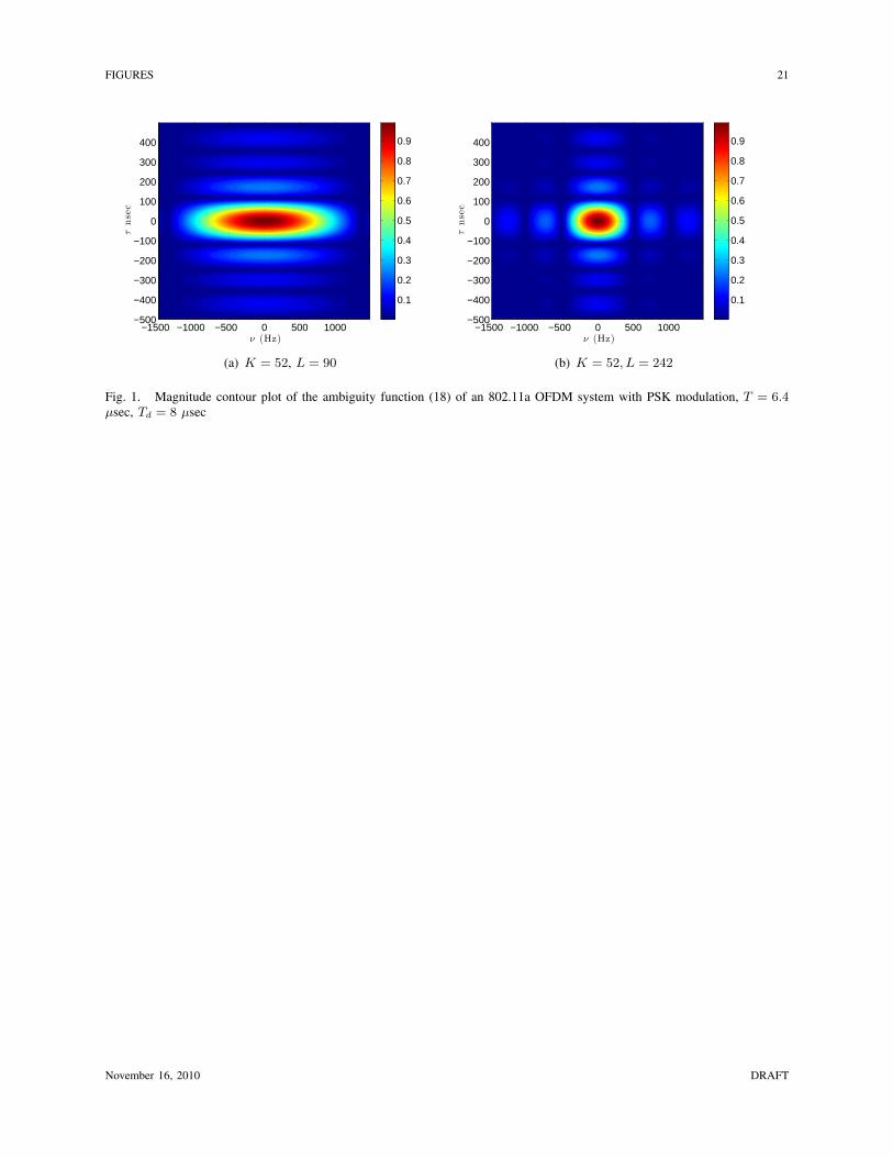
Ax(τ, ν) ≈ e−jπKτ/T cos [π(K/2 + 1)(τ/T )] sinc(πτK/(2T ))sinc(πνTdL) (18)

From the above expressions (17) and (18), we see that the sinc terms introduce sidelobes in

the ambiguity function. Interestingly, the sidelobes are de-coupled in time and frequency. As an

example, the ambiguity function of the 802.11a standard [34, 35] is plotted in Fig. 1, i.e. K = 53

subcarriers, with a null subcarrier at k = bK/2c + 1, Td = 8 µsec and T = 6.4 µsec. From

Fig. 1, as predicted by (18) we see that increasing L improves the Doppler resolution, but not

the delay resolution, which is dependent only on K and the subcarrier spacing (1/T ).

IV. MULTIPATH PARAMETER ESTIMATION

Our primary objective is to estimate a = (a1, . . . , aP ), τ = (τ1, . . . , τP ) and ν = (ν1, . . . , νP )

in (1) from the received noisy symbols Y (6) given perfect knowledge of X . In this section,

without loss of generality, for brevity of notation, we assume the OFDM system has no null

subcarriers, i.e. K = ∅. Using (12), the maximum likelihood (ML) approach is to solve the

following

(a, τ , ν) = arg mina,τ ,ν‖y −Ω(τ ,ν,X)a‖2, (19)

which is a non-linear least squares minimisation problem. The computational complexity can be

reduced by replacing a with its least squares estimate. That is, for a given τ and ν the ML


10

estimate of a is a linear least squares minimisation problem, which has solution [31]

a =(Ω†Ω

)−1Ω†y, (20)

where we have dropped the dependence of X, τ and ν for brevity of notation. Hence substitut-

ing (20) for a in (19) results in the reduced problem

(τ , ν) = arg maxτ ,ν

y†Ω(Ω†Ω)−1Ω†y. (21)

It is known that problems (21) and (19) are equivalent, i.e. (21) followed by (20) is also the ML

solution [26, 36]. Unfortunately, (21) is in general multimodal, rendering the multidimensional

search for a global extremum computationally prohibitive.

Before we begin our reduced complexity suboptimal solution, let us first make some interesting

observations about (21). Let R = Ω†Ω and w = Ω†y. From (13), it is straightforward to show,

Rij = KLAx(τi − τj, νj − νi) (22)

wi = ψ†(νi) (Y X∗)φ(τi), (23)

for i, j = 1, . . . , P , where ψ(νi) and φ(τi) denote column i of the matrices Ψ and Φ respectively,

and A∗ denotes the element-wise conjugate of the matrix A. Thus, rather than performing com-

putation of R = Ω†Ω (requiring on the order of PKL(KL+1)/2 complex multiply-accumulate

operations) using standard matrix operations, to reduce complexity, R can be evaluated using the

ambiguity function via a look-up table. Moreover, for the special case of PSK modulation, (17)

implies we only need the evaluation of a sinc(x) function.

For the special case of P = 1, the ML solution (21) becomes

(τ1, ν1) = arg maxτ,ν

∣∣ψ†(ν1) (Y X∗)φ(τ1)∣∣2 , (24)

after which the corresponding complex gain ML estimates can be determined using (20),

a1 =1

KLψ†(ν1) (Y X∗)φ(τ1). (25)

We see that the solution to (21) corresponds to the maximum absolute value of the 2-D peri-

odogram [37]. Moreover, the CRLB for the estimation of a single tap multipath channel can be

written as [24]

var[ν1Td] ≥1

4π2

6

KL(L2 − 1)

σ2

|a1|2, var [τ1/T ] ≥ 1

4π2

6

KL(K2 − 1)

σ2

|a1|2. (26)


11

Note that Kay and Nekovei [25] proposed a low complexity weighted phase averager estimator

as an alternative to solving (24).

If we were to use (24) when multiple taps are present (P > 1), then

ψ†(ν) (Y X∗)φ(τ) = KL∑p

apAx(νp − ν, τ − τp) +ψ†(ν) [Z X∗]φ(τ),

which is the superimposition of complex scaled, delay and frequency shifted ambiguity functions,

plus an additive Gaussian noise term. We see that detection and estimation of a particular tap

will be significantly affected by the main lobe and sidelobes from the ambiguity functions of the

remaining taps. This motivates a successive cancellation approach whereby the signal contribution

in Y induced by a multipath tap is removed after it is detected, thus allowing subsequent taps

to be detected and estimated. Successive cancellation algorithms have found widespread use in

a number of communication scenarios requiring the recovery of multiple superimposed signals.

In particular, interference cancellation (successive and parallel forms) is the basis of practical

low-complexity multi-user decoding algorithms, which attain close to single-user bit error rate

performance [38]. In our case, the superimposed signals are not signals from multiple users,

but time/frequency shifted versions of the same signal. However the same principle can still be

applied, and as we will see later, achieves performance close to the CRLB of a single tap channel

(provided the taps are sufficiently separated in either delay or Doppler). In this direction, the

first algorithm we propose is based on successive cancellation and is employed to find an initial

estimate of the delay, Doppler and complex gain of each tap. The second algorithm we propose

is based on parallel cancellation and is employed to refine the initial estimates. Integral to both

of these algorithms is a search for the largest absolute value of a 2-D periodogram [37], and

we propose a low-complexity 2-D bisection algorithm for doing this. A detailed description of

each of these algorithms is given as follows.

A. Initial Estimation

Algorithm 1 describes our proposed initial successive cancellation procedure. First we initialise

the residual error matrix E(1) equal to the received noisy OFDM symbols Y . At iteration

p = 1, 2, . . . , P : we find τp and νp that correspond to the maximum absolute value squared of


12

the 2-D periodigram of E(p); construct the p× p matrix

R(p) =

R11 R12 . . . R1p

... . . .

Rp1 Rp2 . . . Rpp

and length p vector w(p) = (w1, w2, . . . , wp) substituting the delay and Doppler estimates τ (p) =

(τ1, . . . , τp) and ν(p) = (ν1, . . . , νp) into (22) and (23); re-estimate the length p complex gain

vector a(p) = (a1 . . . , ap) = (R(p))−1w(p); and finally subtract the signal contributions of all p

estimated multipath components from Y , which becomes the residual error matrix for the next

iteration.

Typically Algorithm 1 will estimate the multipath starting from the strongest to the weakest

tap, i.e. |a1| > |a2| > . . . > |aP |. Thus, for the case when P is unknown, an obvious exit

criterion is to stop once |ap| < γ, where γ is a threshold that determines the minimum tap

energy. Alternatively, the Algorithm can be modified to incorporate a model order selection

rule [29].

Note that two simple modifications can be made to Algorithm 1 to further reduce complexity.

Firstly, in the main loop, rather than subtracting all multipath contributions of the previously

estimated components from the original signal Y to obtain the residual errorE(p), simply subtract

the contribution of the current estimate from the residual error of the previous iteration E(p−1),

i.e. line 6 can be replaced with E(p) = E(p−1) −[a

(p)p ψ(νp)φ

†(τp)] X . Secondly, rather

than operating on Y , one could apply the algorithm on the zero-forcing estimate of H , i.e.

Hl,k = Yl,kX∗l,k/|Xl,k|. Thus, in Algorithm 1, one simply replaces Y with H and the Hadamard

product with X in lines 3 and 6 is no longer required. To summarize, we can make the following

complexity-reducing modifications to Algorithm 1. Line 1: E(1) = H , Line 3: (τp, νp) =

arg maxτ,ν

∣∣∣ψ†(ν)E(p)φ(τ)∣∣∣2, and Line 6: E(p+1) = H −

[Ψ(ν(p))diag(a(p))Φ†(τ (p))

]B. Estimation Refinement

It is quite reasonable to rely solely on Algorithm 1 to estimate the delay/Doppler. Indeed

similar approaches have been employed in [14, 15, 28], but without any detailed comparison to

theoretical bounds. We find that the performance of Algorithm 1 is hampered by interference from

undetected taps, which as we will see later, introduces a floor in the root mean squared (RMS)


13

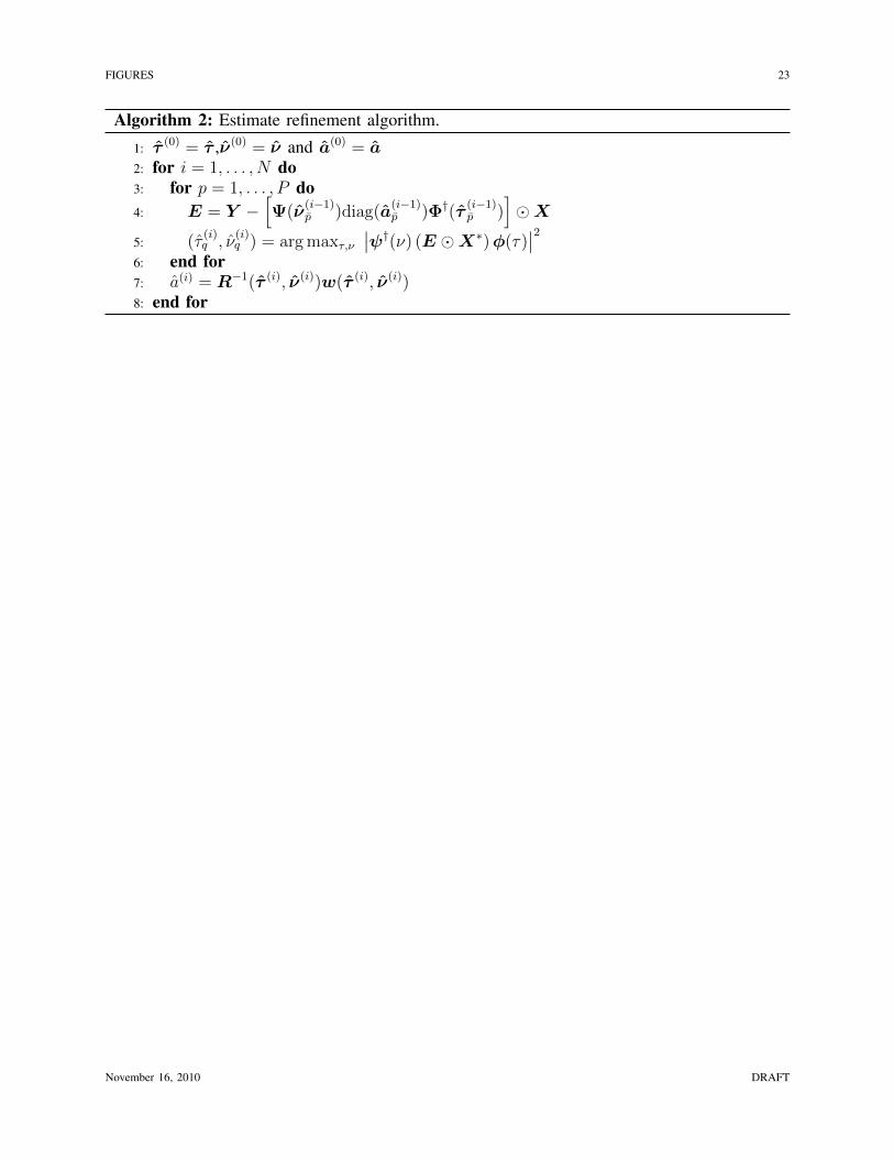
error performance. Therefore we propose a refinement process based on parallel cancellation

whereby for each iteration, all multipath components are removed except for the component of

interest, that is subsequently re-estimated. This refinement procedure is described in detail in

Algorithm 2, where τ (i) = (τ(i)1 , . . . , τ

(i)P ), ν(i) = (ν

(i)1 , . . . , ν

(i)P ) and a(i) = (a

(i)1 , . . . , a

(i)P ) denote

the refined estimates after the i’th iteration, and τ (0) = τ , ν(0) = ν and a(0) = a are the initial

estimates obtained from Algorithm 1. In addition, we let τ (i)p , ν(i)

p and a(i)p denote the refined

estimates at step i with element p element omitted.

Note that rather than refining for a fixed number of iterations, Algorithm 2 can be easily be

modified to incorporated an early stopping criterion, e.g. by checking the improvement in the

residual error ‖E‖2. As previously described for Algorithm 1, one could apply Algorithm 2 to

the zero-forcing estimate of H , i.e. replace Y with H and removing the Hadamard product

with X in lines 4 and 5.

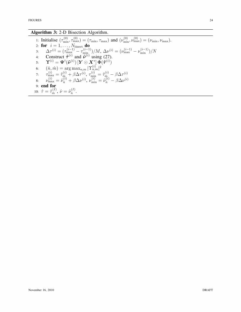
C. 2-D Bisection Algorithm

As mentioned earlier, the maximisation step in line 3 Algorithm 1 and line 5 of Algorithm 2

can be solved by finding the maximum absolute value of the 2-D periodogram [37]. To perform

this operation, we propose a 2-D bisection approach described as follows. First we assume

τp ∈ (τmin, τmax) and νp ∈ (νmin, νmax) for all p = 1, . . . , P , i.e. the delay/Doppler of each tap is

constrained to lie within predefined intervals. Let (τ(i)min, τ

(i)max) and (ν

(i)min, ν

(i)max) denote the search

interval at iteration i, and τ (i) and ν(i) denote linearly spaced vectors within these intervals, i.e.

τ (i)m = τ

(i)min + (m− 1)∆τ (i) ν(i)

m = ν(i)min + (n− 1)∆ν(i), (27)

for m = 1, . . . ,M and n = 1, . . . , N , where ∆τ (i) = (τ(i)max − τ (i)

min)/M and ∆ν(i) = (ν(i)max −

ν(i)min)/N denote the bin spacing at the i’th iteration. For each iteration of the bisection algorithm,

we find the indices corresponding to the largest peak of Ψ†(ν(i)) [Y X∗] Φ(τ (i)). For the

next iteration, the search interval is then bisected or reduced to a smaller 2-D region, i.e.(2β∆τ (i), 2β∆ν(i)

), centered at the previous delay/Doppler indices (typically β ≥ 1/2). A

detailed description of the procedure is given in Algorithm 3. Note that for ease of exposition, the

bisection process completes after a fixed number of iterations Nbisect. The algorithm can easily

be modified to employ an early stopping criterion, e.g. exit the main loop when ∆τ (i) < ετ and

∆ν(i) < εν to ensure a certain level of delay/Doppler resolution.


14

V. PERFORMANCE EVALUATION

Performance evaluation is complicated by the fact there are infinitely many possible multipath

channel realisations and many OFDM system design configurations all of which can have a

significant effect on the estimator’s performance. To reduce our analysis, we focus on OFDM

systems with similar specifications to the IEEE802.11p standard (as described in Section III).

In addition, we concentrate on multipath channels typical of outdoor mobile vehicular environ-

ments [39], i.e. delay spreads not exceeding 200 nsec and Doppler differentials not exceeding

1000 Hz. For example, at a carrier frequency of 5.9 GHz, this corresponds to a maximum excess

delay of 60 m and velocity differentials of 51 m/s or 183 km/hr.

Ultimately, we would like to investigate the estimator’s performance for as many different

multipath channel configurations as possible. However, we find that the performance is signifi-

cantly affected by the location of the multipath taps in the 2-D delay/Doppler space. When two

or more taps are too close to each other there is a high probability Algorithm 1 will detect these

as a single tap.1 The minimum separation distance is essentially the delay/Doppler resolution of

the estimator, which is dependent on the main lobe of the ambiguity function, which in turn, is

dependent on the subcarrier spacing and duration of the OFDM packet (as evidenced in (17)).

When the components are sufficiently separated, the estimator’s performance is dominated by

AWGN and hence the CRLB (26).

To separate the above mentioned effects, we conducted Monte Carlo simulations whereby for

each trial a random set of multipath taps is generated. Whilst these taps are drawn randomly, they

are not i.i.d., and instead are drawn to ensure a minimum separation in delay and Doppler. This

is achieved by continually drawing a vector of P delays from an i.i.d. uniform distribution on

the interval (τmin, τmax) until the minimum pairwise distance between the delays is greater than a

specified ∆τ . The delays are then sorted in ascending order. The Doppler offsets are generated in

a similar fashion on the interval (νmin, νmax), but with no sorting. Note that ∆τ ≤ (τmax−τmin)/P

and similarly ∆ν ≤ (νmax − νmin)/P . Whilst we fix the power delay profile, for each trial, the

phase of each tap is generated randomly according to a uniform distribution over the interval

(0, 2π). Once the multipath taps are generated, the frequency domain channel coefficients are

1In a physical sense, if these closely spaced taps are the result of first order reflections it may imply they are reflections from

the same object.


15

generated using (8) and the received noisy symbols are generated using (7), where, without loss

of generality, we assume Xl,k = 1. It is important to note how the error statistics were calculated.

For each trial, RMS error statistics were only collected when all taps are detected, i.e. each tap is

closest (in Euclidean distance) to a single estimate. Events when this does not occur are counted

as missed detections, but are not included in the RMS error statistics. This allows us to separate

error events caused by miss detections due to the transmit ambiguity function.

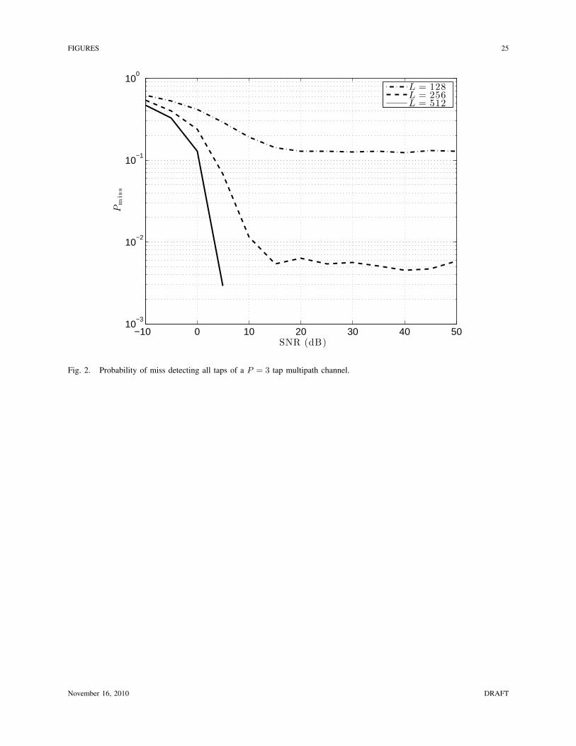
In our simulations we considered a P = 3 tap multipath channel, with power delay profile

|a1|2 = 0, |a2|2 = −10 and |a3|2 = −20 dB, (τmin, τmax) = (0, 200) nsec, (νmin, νmax) =

(−500, 500), minimum delay separation of ∆τ = 66.67 nsec and minimum Doppler separation

of ∆ν = 333.33 Hz. Error statistics were collected from 104 trials.

Fig. 2 shows the miss detection probability for L = 128, 256 and 512 OFDM packet lengths.

We see that when L = 128, the miss detection probability is greater than 10 percent. As L

increases the main lobe of the ambiguity function shrinks in the Doppler domain improving the

resolution of the estimator and hence reduces the miss detection probability. When L = 512, no

miss detections were recorded for an SNR greater than 5 dB.

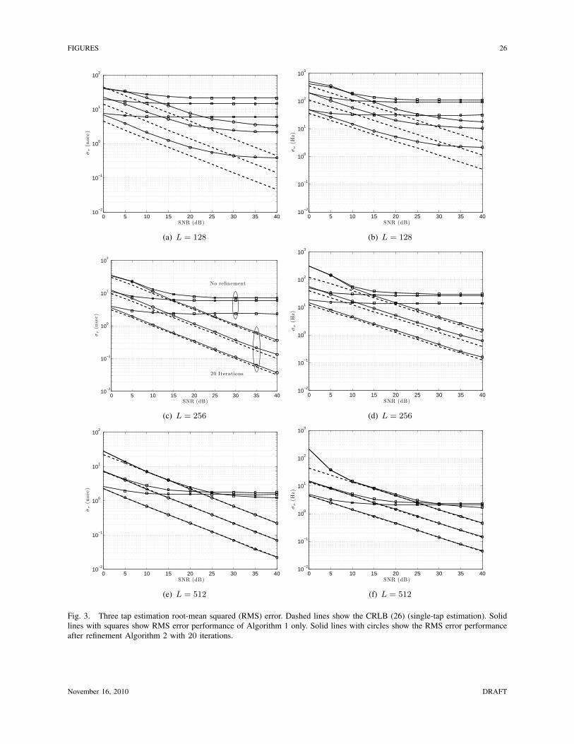
Fig. 3 shows the RMS estimation error results (recalling that this is restricted to instances

where missed detection does not occur). The square marked curves show the RMS error when

no refinement is performed, i.e. only Algorithm 1 is employed. In this case a floor in the RMS

error performance is observed (caused by undetected multipath components in the successive

cancellation process). When refinement is employed, as shown by the circle marked curves, the

error floor is significantly reduced. Moreover, as L increases the floor does not occur until very

high SNRs and the RMS error performance is primarily dominated by the CRLB (26), which

is shown by the dashed curves. Thus with sufficiently long packet length, Algorthms 1 and 2

deliver single-tap performance, i.e. are able to accurately cancel the contributions of “interfering”

taps.

It is interesting to translate the estimator performance into range/velocity resolution. Consid-

ering L = 512 and SNR 20 dB, the 3-standard-deviation values for the −20 dB tap are 9 ns

and 15 Hz. This corresponds to range resolution of 2.7 m and relative velocity resolution (at

5.9GHz) of 0.77 m/s (2.7 km/h). This clearly demonstrates the capability to accurately resolve

quite challenging multipath channels.


16

VI. CONCLUSION

In this paper we examined amplitude, delay and Doppler estimation of the multipath channel

taps from OFDM signal transmission in a doubly selective mobile environment. Under certain

practical system design and mobile channel assumptions, we showed that the frequency domain

channel coefficients for an entire OFDM packet can be written as the superimposition of 2-D

complex sinusoids. The angular frequency of each sinusoid is proportional to the delay and

Doppler of a particular multipath tap.

ML estimation of the delay/Doppler requires non-linear least squares minimisation, which is

computationally infeasible for practical implementation. We therefore proposed a low complexity

suboptimal estimation method, based on successive cancellation, whereby multipath components

are removed once they are detected. The complexity reduction results from a simplification

of the channel model, where time variations manifest only as Doppler frequency offsets for

each tap. For a single tap channel, this method is maximum likelihood. The performance of

this successive cancellation approach can be degraded by interference from taps that are yet to

be detected in future iterations. To remedy this, we proposed a refinement algorithm based on

parallel cancellation, i.e. all estimated multipath components are subtracted except the component

of interest, which is subsequently re-estimated.

The performance of our estimator was shown to be dominated by two effects: separation of the

multipath taps in the delay/Doppler plane; and noise. When two or more taps are close together

in the 2-D delay/Doppler space, the estimator may detect these as single tap, resulting in missed

detections and significantly degrading the RMS error of other detected taps. When the multipath

taps are sufficiently separated in delay/Doppler the estimator performance is dominated by noise

and hence the RMS error of the refined estimates are very close the CRLB of a single 2-D

sinusoid in additive white Guassian noise. We believe the missed detections are caused by the

transmit ambiguity function: broadness of the main lobe affects the delay/Doppler resolution;

and sidelobes of components that have not been sufficiently subtracted can mask weaker taps.

However, a detailed analytic investigation of these effects is beyond the scope of this paper and

the subject of future work.

Note that although our results assume delay spreads less than the cyclic prefix, our proposed

estimator still works well without this restriction. Multipath taps with delay exceeding the cyclic


17

prefix will introduce inter-symbol interference. The estimator views this interference as extra

noise on the received symbols. Thus, as long as AWGN dominates, this extra interference will

have negligible effect on performance.

APPENDIX I

DERIVATION OF RECEIVER MATCHED FILTER OUTPUT

For clarity we repeat the transmitted signal,

x(t) =∑l′

xl′(t) =1√KL

∑l′,k′

Xl′,k′w(t− (l′ − 1)Td)ej2π(k′−1−bK/2c)(t−Tcp)/T . (28)

Application of the channel response (4) to the transmitted signal (28) yields

y(t) = x(t) ∗ h(t, τ) + z(t) =

∫ ∞−∞

x(t− τ)h(t, τ) dτ

=1√KL

∑l′,k′,p

apXl′,k′

∫ ∞−∞

g(τ − τp)w(t− τ − (l′ − 1)Td)e−2πνptej2π(k′−1−bK/2c)(t−τ−Tcp)/T dτ + z(t)

=1√KL

∑l′,k′,p

apXl′,k′e−j2π(k′−1−bK/2c)Tcp/T e

−j2π(νp− k′−1

T+ K

2T

)tsl′,k′(t, τp) + z(t), (29)

where the integral

sl′,k′(t, τp) =

∫ ∞−∞

g(τ − τp)e−j2π(k′−1−bK/2c)τ/Tw(t− τ − (l′ − 1)Td) dτ, (30)

is simply the convolution of a time/frequency translated filter response g(t) and time shifted

window function w(t). Using the appropriate properties of Fourier transforms, the Fourier

transform of (30) can be written as

Sl′,k′(f, τp) = e−j2πτp

[k′−1T− K

2T+f]e−j2πf(l′−1)TdG

(f +

k′ − 1

T− K

2T

)W (f), (31)

where G(f) and W (f) denote the Fourier transforms of g(t) and w(t) respectively. In prac-

tical OFDM systems the passband bandwidth of G(f) is typically greater than K/T and the

bandwidth of W (f) is typically less than 1/T , e.g. for the simple case w(t) = 1√Td

, then

W (f) =√Tde

−jπfTdsinc(πfTd). Moreover, in many OFDM standards the outer subcarriers are

null subcarriers. Hence assuming negligible passband ripple then G(f + k′−1

T− K

2T

)≈ 1 for

k′ = 1, . . . , K and |f | < 1/(2T ). Therefore,

Sl′,k′(f, τp) ≈ e−j2πτp

[k′−1T− K

2T+f]e−j2πf(l′−1)TdW (f). (32)


18

Thus, taking the inverse Fourier transform yields

sl′,k′(t, τp) ≈ e−j2πτp

[k′−1T− K

2T

] ∫ ∞−∞

W (f)ej2πf [t−τp−(l′−1)Td] df

= e−j2πτp

[k′−1T− K

2T

]w(t− τp − (l′ − 1)Td). (33)

Substituting (33) into (29) gives,

y(t) =1√KL

∑l′,k′,p

apXl′,k′e−j2π(k′−1−bK/2c)Tcp/T e

−j2π(νp− k′−1

T+ K

2T

)t

× e−j2πτp(

k′−1T− K

2T

)w(t− τp − (l′ − 1)Td) + z(t), (34)

The receiver now performs the matched filter to the transmitted sinusoids (less the cyclic

prefix), i.e.

Yl,k =1√KL

∫ lTd

Tcp+(l−1)Td

y(t)w∗(t− lTd)e−j2π(k−1−bK/2c)(t−Tcp)/T dt

=1

KL

∑l′,k′,p

apXl′,k′e−j2πτp

(k′−1T− K

2T

)e−j2π(k′−k)Tcp/T

×∫ lTd

Tcp+(l−1)Td

w(t− τp − (l′ − 1)Td)w∗(t− (l − 1)Td)e

−j2π(νp+ k−k′

T

)tdt+ Zl,k

=1

KL

∑l′,k′,p

apXl′,k′e−j2πτp

(k′−1T− K

2T

)e−j2π(k′−k)Tcp/T e

−j2π(νp+ k−k′

T

)(l−1)Td

× Aw(τp + (l′ − l)Td, νp +

k − k′

T

)+ Zl,k, (35)

where

Aw(τ, ν) =

∫ Td

Tcp

w(t− τ)w∗(t)e−j2πνt dt, (36)

which resembles the ambiguity function of w(t).2 In practical OFDM systems, usually maxp τp <

Tcp and maxp νp 1/T and the windowing function is usually designed such that

Aw(τp + (l′ − l)Td, νp + k−k′

T

)≈ 0 for k 6= k′ or l 6= l′. Hence we may write,

Yl,k =1

KL

∑p

apXl,ke−j2πτp( k−1

T− K

2T )e−j2πνpTd(l−1)Aw(τp, νp) + Zl,k

=1

KL

∑p

apXl,ke−j2π(k−1)τp/T e−j2π(l−1)νpTd + Zl,k, (37)

2The function Aw(τ, ν) is not quite the ambiguity function of w(t) because of the limits of integration.


19

where ap = e−jπKτp/T Aw(τp, νp). With some slight abuse of notation, for the remainder of the

paper for brevity of notation (and without loss of generality) we will replace ap with ap. Defining

Hl,k according to (8), we obtain (7).

REFERENCES

[1] J. G. Proakis, Digital Communications, McGraw-Hill, 4 edition, 2000.

[2] A. Goldsmith, Wireless Comunications, Cambridge University Press, 2005.

[3] A. Peled and A. Ruiz, “Frequency domain data transmission using reduced computational complexity algorithms,” in Int.

Conf. on Acoustics, Speech, and Sig. Proc., Apr 1980, vol. 5, pp. 964–967.

[4] L. Cimini, “Analysis and simulation of a digital mobile channel using orthogonal frequency division multiplexing,” IEEE

Trans. Commun., vol. 33, no. 7, pp. 665–675, Jul. 1985.

[5] R. van Nee and R. Prasad, OFDM for Wireless Multimedia Communications, Artech House Publishers, 1999.

[6] R. van Nee, V. K. Jones, G. Awater, A. van Zelst, J. Gardner, and G. Steele, “The 802.11n MIMO-OFDM standard for

wireless LAN and beyond,” Wireless Personal Commun., vol. 37, pp. 445–453, 2006.

[7] G. Hiertz, D. Denteneer, L. Stibor, Y. Zang, X.P. Costa, and B. Walke, “The IEEE 802.11 universe,” IEEE Commun.

Mag., vol. 48, no. 1, pp. 62 –70, Jan. 2010.

[8] “802.11p-2010 IEEE standard for information technology – Telecommunications and information exchange between

systems – Local and metropolitan area networks – Specific requirements part 11: Wireless LAN medium access control

(MAC) and physical layer (PHY) spec,” 2010.

[9] D. Haley P. Alexander and A. Grant, “Cooperative intelligent transport systems: 5.9 GHz field trials,” Submitted to Proc.

IEEE, 2010.

[10] W. Kozek and A. F. Molisch, “Nonorthogonal pulseshapes for multicarrier communications in doubly dispersive channels,”

IEEE J. Sel. Areas Commun., vol. 16, no. 8, pp. 1579–1589, Oct. 1998.

[11] K. Liu, T. Kadous, and A. M. Sayeed, “Orthogonal time-frequency signaling over doubly dispersive channels,” IEEE

Trans. Inform. Theory, vol. 50, no. 11, pp. 2583–2603, Nov 2004.

[12] G. Taubock and F. Hlawatsch, “On the capacity-achieving input covariance for multicarrier communications over doubly

selective channels,” in IEEE Int. Symp. Inform. Theory, 2007.

[13] J Karedal, F Tufvesson, N Czink, A Paier, C Dumard, T Zemen, C Mecklenbrauker, and A Molisch, “A geometry-based

stochastic MIMO model for vehicle-to-vehicle communications,” IEEE Trans. Wireless Commun., vol. 8, no. 7, pp. 3646

– 3657, Jul 2009.

[14] T. A. Thomas, T. P. Krauss, and F. W. Vook, “CHAMPS: A near-ML joint Doppler frequency/ToA search for channel

characterization,” in IEEE Vehic. Technol. Conf., 6-9 Oct. 2003, pp. 74–78.

[15] C. R. Berger, S. Zhou, and P. Willett, “Signal extraction using compressed sensing for passive radar with OFDM signals,”

in 11th International Conference on Information Fusion, Jan 2008, pp. 1 – 6.

[16] M. Cherniakov and D. V. Nezlin, Bistatic radar: principles and practice, John Wiley, Chichester, 2007.

[17] E. J. Candes and M. B. Wakin, “An introduction to compressive sampling,” IEEE Signal Processing Magazine, vol. 21,

no. 2, Mar 2008.

[18] D. Needell and R. Vershynin, “Uniform uncertainty principle and signal recovery via regularized orthogonal matching

pursuit,” http://arxiv.org/pdf/0707.4203v4, Mar 2008.


20

[19] D. Needell, J. Tropp, and R. Vershynin, “Greedy signal recovery review,” in Asilomar Conf. on Signals Systems and

Computers, Oct. 2008, pp. 1048–1050.

[20] G. Taubock and F. Hlawatsch, “A compressed sensing technique for ofdm channel estimation in mobile environments:

expoiting channel sparsity for reducing pilots,” in IEEE Int. Conf. on Accoustics Speach and Signal Proc., 2008.

[21] G. Taubock, F. Hlawatsch, D. Eiwen, and H. Rauhut, “Compressive estimation of doubly selective channels in multicarrier

systems: Leakage effects and sparisty-enhancing processing,” IEEE J. Sel. Topics in Sig. Proc., vol. 4, no. 2, pp. 255–271,

Apr. 2010.

[22] I. C. Wong and B. L. Evans, “Sinusoidal modeling and adaptive channel prediction in mobile OFDM systems,” IEEE

Trans. Sig. Proc., vol. 56, no. 4, pp. 1601–1615, Apr. 2008.

[23] I. C. Wong and B. L. Evans, “Joint channel estimation and prediction OFDM systems,” in IEEE GLOBECOM, St. Louis,

MO, Dec. 2005, p. 2259.

[24] H. Chien, 2-D estimation from AR models, Ph.D. thesis, Univ. of Rhode Island, Kingston, RI, May 1981.

[25] S. Kay and R. Nekovei, “An efficient two-dimensional frequency estimator,” IEEE Trans. Acoustics, Speech and Sig.

Proc., vol. 38, no. 10, pp. 1807–1810, Oct 1990.

[26] Y. Bresler and A. Macovski, “Exact maximum likelihood parameter estimation of superimposed exponential signals in

noise,” IEEE Trans. Acoustics, Speech and Sig. Proc., vol. 34, no. 5, pp. 1081–1089, Oct. 1986.

[27] C. Rao, L. Zhao, and B. Zhou, “Maximum likelihood estimation of 2-D superimposed exponential signals,” IEEE Trans.

Sig. Proc., vol. 42, no. 7, pp. 1795–1802, July 1994.

[28] M. Kliger and J. M. Francos, “MAP model order selection rule for 2-D sinusoids in white noise,” IEEE Trans. Sig. Proc.,

vol. 53, no. 7, pp. 2563–2575, July 2005.

[29] P. Stoica and Y. Selen, “Model-order selection: a review of information criterion rules,” IEEE Sig. Proc. Mag., pp. 36–47,

2004.

[30] V. Pereyra, “Iterative methods for solving nonlinear least squares problems,” SIAM J. Numer. Anal., vol. 4, no. 1, pp.

27–36, Mar. 1967.

[31] S. Boyd and L. Vandenberghe, Convex Optimization, Cambridge University Press, 2004.

[32] M. Skolnik, Introduction to Radar Systems, McGraw-Hill, New York, 3rd edition, 2002.

[33] R. Horn and C. R. Johnson, Matrix Analysis, Cambridge University Press, 1985.

[34] IEEE 802.11a-1999, “Supplement to IEEE Standard for Information Technology - Telecommunications and Information

Exchange Between Systems - Local and Metropolitan Area Networks - Specific Requirements. Part 11: Wireless LAN

Medium Access Control (MAC) and Physical Layer (PHY) Specifications: High-Speed Physical Layer in the 5 GHz Band,”

1999.

[35] B. O’Hara and A. Petrick, The IEEE 802.11 Handbook: A Designer’s Companion, IEEE Press, 1999.

[36] G. H. Golub and V. Pereyra, “The differentiation of psuedo-inverses and non-linear least squares problems whose variables

separate,” SIAM J. Numer. Anal., vol. 10, no. 2, pp. 413–432, Apr. 1973.

[37] S. M. Kay, Modern spectral estimation: theory and application, Prentice Hall, Englewood Cliffs, N.J., 1988.

[38] C. Schlegel and A. Grant, Coordinated Multiuser Communications, Springer, 2006.

[39] P. Alexander, D. Haley, and A. Grant, “Outdoor mobile broadband access with 802.11,” IEEE Commun. Mag., vol. 45,

no. 11, pp. 108–114, Nov. 2007.


FIGURES 21

ν (Hz)

τnsec

−1500 −1000 −500 0 500 1000−500

−400

−300

−200

−100

0

100

200

300

400

0.1

0.2

0.3

0.4

0.5

0.6

0.7

0.8

0.9

(a) K = 52, L = 90

ν (Hz)

τnsec

−1500 −1000 −500 0 500 1000−500

−400

−300

−200

−100

0

100

200

300

400

0.1

0.2

0.3

0.4

0.5

0.6

0.7

0.8

0.9

(b) K = 52, L = 242

Fig. 1. Magnitude contour plot of the ambiguity function (18) of an 802.11a OFDM system with PSK modulation, T = 6.4µsec, Td = 8 µsec


FIGURES 22

Algorithm 1: Initial estimation via successive cancellation.

1: E(1) = Y2: for p = 1, . . . , P do3: (τp, νp) = arg maxτ,ν

∣∣∣ψ†(ν)(E(p) X∗

)φ(τ)

∣∣∣24: Contruct R(p) and w(p) using (22) and (23) with τ1, . . . , τp and ν1, . . . , νp.5: a(p) = (R(p))−1w(p)

6: E(p+1) = Y −[Ψ(ν(p))diag(a(p))Φ†(τ (p))

]X

7: end for


FIGURES 23

Algorithm 2: Estimate refinement algorithm.

1: τ (0) = τ ,ν(0) = ν and a(0) = a2: for i = 1, . . . , N do3: for p = 1, . . . , P do4: E = Y −

[Ψ(ν

(i−1)p )diag(a

(i−1)p )Φ†(τ

(i−1)p )

]X

5: (τ(i)q , ν

(i)q ) = arg maxτ,ν

∣∣ψ†(ν) (E X∗)φ(τ)∣∣2

6: end for7: a(i) = R−1(τ (i), ν(i))w(τ (i), ν(i))8: end for


FIGURES 24

Algorithm 3: 2-D Bisection Algorithm.

1: Initialise (τ(0)min, τ

(0)max) = (τmin, τmax) and (ν

(0)min, ν

(0)max) = (νmin, νmax).

2: for i = 1, . . . , Nbisect do3: ∆τ (i) = (τ

(i−1)max − τ (i−1)

min )/M , ∆ν(i) = (ν(i−1)max − ν(i−1)

min )/N4: Construct τ (i) and ν(i) using (27).5: Υ(i) = Ψ†(ν(i)) [Y X∗] Φ(τ (i))

6: (n, m) = arg maxn,m |Υ(i)n,m|2

7: τ(i)max = τ

(i)m + β∆τ (i), τ (i)

min = τ(i)m − β∆τ (i)

8: ν(i)max = ν

(i)n + β∆ν(i), ν(i)

min = ν(i)n − β∆ν(i)

9: end for10: τ = τ

(I)m , ν = ν

(I)n .


FIGURES 25

−10 0 10 20 30 40 5010

−3

10−2

10−1

100

SNR (dB)

Pm

iss

L = 128L = 256L = 512

Fig. 2. Probability of miss detecting all taps of a P = 3 tap multipath channel.


FIGURES 26

0 5 10 15 20 25 30 35 4010

−2

10−1

100

101

102

SNR (dB)

στ(n

sec)

(a) L = 128

0 5 10 15 20 25 30 35 4010

−2

10−1

100

101

102

103

SNR (dB)

σν(H

z)

(b) L = 128

0 5 10 15 20 25 30 35 4010

−2

10−1

100

101

102

SNR (dB)

στ(n

sec)

No refinement

20 Iterations

(c) L = 256

0 5 10 15 20 25 30 35 4010

−2

10−1

100

101

102

103

SNR (dB)

σν(H

z)

(d) L = 256

0 5 10 15 20 25 30 35 4010

−2

10−1

100

101

102

SNR (dB)

στ(n

sec)

(e) L = 512

0 5 10 15 20 25 30 35 4010

−2

10−1

100

101

102

103

SNR (dB)

σν(H

z)

(f) L = 512

Fig. 3. Three tap estimation root-mean squared (RMS) error. Dashed lines show the CRLB (26) (single-tap estimation). Solidlines with squares show RMS error performance of Algorithm 1 only. Solid lines with circles show the RMS error performanceafter refinement Algorithm 2 with 20 iterations.


Documents

1 Multipath Parameter Estimation from OFDM Signals in ... · PDF file1 Multipath Parameter Estimation from OFDM Signals in Mobile Channels Nick Letzepis, Member, IEEE, Alex Grant,