Embed Size (px)
Citation preview

1
Movement patterns of the European squid Loligo vulgaris during the inshore 1
spawning season 2
3
4
Miguel Cabanellas-Reboredo1,*, Josep Alós1, Miquel Palmer1, David March1 and 5
Ron O’Dor2 6
7
RUNNING HEAD: Movement patterns of Loligo vulgaris 8
9
10
1Instituto Mediterráneo de Estudios Avanzados, IMEDEA (CSIC-UIB), C/ Miquel Marques 21, 07190 11
Esporles, Islas Baleares, Spain. 12
2Biology Department of Dalhousie University, Halifax, Nova Scotia Canada, B3H 4J1. 13
*corresponding author: E-mail: [email protected], telephone: +34 971611408, fax: +34 14
971611761. 15

2
ABSTRACT: 16
The European squid Loligo vulgaris in the Western Mediterranean is exploited by both 17
commercial and recreational fleets when it spawns at inshore waters. The inshore 18
recreational fishery in the southern waters Mallorca (Balearic Islands) concentrates 19
within a narrow, well-delineated area and takes place during a very specific period of 20
the day (sunset). Another closely related species, Loligo reynaudii, displays a daily 21
activity cycle during the spawning season (“feeding-at-night and spawning-in-the-day”). 22
Here, the hypothesis that L. vulgaris could display a similar daily activity pattern has 23
been tested using acoustic tracking telemetry. Two tracking experiments during May-24
July 2010 and December 2010-March 2011 were conducted, in which a total of 26 squid 25
were tagged. The results obtained suggested that L. vulgaris movements differ between 26
day and night. The squid seem to move within a small area during the daytime but it 27
would cover a larger area from sunset to sunrise. The probability of detecting squid was 28
greatest between a depth of 25 and 30 m. The abundance of egg clutches at this depth 29
range also seemed to be greater. The distribution of the recreational fishing effort using 30
line jigging, both in time (at sunset) and in space (at the 20-35-m depth range), also 31
supports the “feeding-at-night and spawning-in-the-day” hypothesis. 32
33
KEYWORDS: Acoustic telemetry · Daily activity cycle · Recreational fishing effort · 34
Egg clutch distribution 35
3
INTRODUCTION 36
The European squid Loligo vulgaris Lamarck (1798) is targeted in the Mediterranean 37
Sea by both commercial and recreational fishers (Guerra et al. 1994, González & 38
Sánchez 2002, Morales-Nin et al. 2005). This species experiences large fishing pressure 39
and has a high socio-economical value (Guerra et al. 1994, Ulaş & Aydin 2011). 40
Most of the life-history traits of this species are known (Guerra 1992, Guerra & Rocha 41
1994, Moreno et al. 2002, Šifner & Vrgoc 2004, Moreno et al. 2007). However, 42
knowledge on the spatial and temporal pattern of habitat use by this species is still 43
scarce and remains elusive, despite the relevance of such knowledge for assessing and 44
managing fishery resources (Pecl et al. 2006, Botsford et al. 2009). 45
One of the movement patterns that has potential outcomes on fishing success is the in-46
offshore seasonally periodical movement. This type of movement has been repeatedly 47
described and related to reproduction and feeding cycles in other cephalopods 48
(Tinbergen & Verwey 1945, Worms 1983, Boyle et al. 1995), and it has been suggested 49
that L. vulgaris would display this pattern (Sánchez & Guerra 1994, Šifner & Vrgoc 50
2004). Large mature or pre-mature individuals are abundant at shallow coastal waters, 51
seemingly for mating and spawning; the new recruits seems to hatch near the coast and 52
subsequently migrate towards deeper waters (Guerra 1992, Sánchez & Guerra 1994). 53
The outcome of such an abundance pattern is the development of a seasonal fishery for 54
L. vulgaris when large squid are abundant close to shore. Nearshore spawning 55
aggregations of other Loligo species are typically exploited using line jigging (Augustyn 56
& Roel 1998, Hanlon 1998, Iwata et al. 2010, Postuma & Gasalla 2010). In inshore 57
waters near Mallorca Island, other commercial gears, including seine and trammel nets, 58
can sporadically capture squid as very valued bycatch (Cabanellas-Reboredo et al. 59
2011). However, the main gear used when targeting squid is line jigging, which is 60

4
extensively used by both commercial (artisanal) and recreational fishers (Guerra et al. 61
1994; Cabanellas-Reboredo et al. 2011). The handline jigging method used by the 62
artisanal fleet typically takes place at fishing grounds located between 20 and 35 m in 63
depth, at night and with the use of lights. Recreational fishers use line jigging at the 64
same fishing grounds but only at sunset (Cabanellas-Reboredo et al. 2011). The use of 65
light is forbidden for the recreational fleet. However, recreational fishers also fish squid 66
after sunset by trolling, but only in very shallow waters (Cabanellas-Reboredo et al. 67
2011) close to the illuminated shore of Palma city, between the shore and a depth of 10 68
m. 69
The specific goal of this study was to use acoustic tracking telemetry for 1) providing 70
the first description of the movement of L. vulgaris during the inshore spawning period 71
and 2) relating such a movement pattern with the spatiotemporal distribution of the 72
fishing efforts. 73
Acoustic tracking telemetry has already been used for describing the movement patterns 74
of other cephalopods (Stark et al. 2005, Payne & O'Dor 2006; Semmens et al. 2007, 75
Dunstan et al. 2011) and for understanding the environmental cues of squid movements 76
(Gilly et al. 2006). In addition, acoustic tracking has been used for describing the 77
relationship between metabolic rate and behavior (O’Dor et al. 1994, O’Dor 2002, 78
Aitken et al. 2005) and for improving fisheries management (Pecl et al. 2006). The 79
movement patterns during spawning aggregations of Loligo reynaudii Orbigny (1845) 80
and their relationship with environmental variability has been demonstrated using 81
acoustic telemetry (Sauer et al. 1997, Downey et al. 2009). 82

5
MATERIALS AND METHODS 83
Experimental design 84
Two acoustic tracking experiments (ATEs) were completed in the southern waters of 85
Mallorca Island (Fig. 1; NW Mediterranean) during the two main spawning seasons of 86
the species (winter and spring-early summer; Guerra & Rocha 1994, Šifner & Vrgoc 87
2004). A preliminary study covering a wide spatial range (ATE1) was carried out 88
between May and July 2010 (Fig. 1A) because no prior information on movement 89
extent was available for L. vulgaris. In accordance with the results obtained in ATE1, a 90
second experiment (ATE2) was completed between December 2010 and March 2011 91
(Fig. 1B). 92
In both of the experiments, an array of omni-directional acoustic receivers 93
(Sonotronics© SUR-1) was deployed (Fig. 1). In ATE1, a wide array distributed along 94
the south of the island was designed to determine the broad scale of the movements 95
(Fig. 1A). The distances between the receivers ranged from 2.6 to 8.9 km. The receivers 96
were placed from 8 m depth (only one receiver) up to 30 m depth (Fig. 1A). A denser 97
array covering only the main fishing grounds in Palma Bay was deployed during ATE2 98
(Fig. 1B). The SURs were placed at the nodes of a 1000 x 1000 m grid. The receivers 99
were placed at depths ranging between 8 to 38 m (Fig. 1B). The number of receivers 100
used was 18 during ATE1 and 17 during ATE2. As probability of detection may be 101
function not only of the distance between receiver and transmitter but also of depth 102
(Claisse et al., 2011), the probability of detection at different distances was estimated at 103
three different depths (10, 30 and 50 m depth) using control tags moored at prefixed 104
distance from the receivers. Detection probability was assumed to follow a binomial 105
distribution and data were fitted to a generalized linear model (GLM, glm function from 106
the R package; depth was considered a categorical factor). 107

6
After the expected battery life of the tags had expired (see details below), we retrieved 108
the receivers and downloaded the data. 109
Acoustic Tagging 110
A total of 26 squid were tagged (Table 1) and released inside the receiver array, with 6 111
individuals during ATE1 and 20 during ATE2 (Fig. 1). Most of the individuals (n=23) 112
were tagged using the miniature tag IBT-96-2 (Sonotronics©). This transmitter measures 113
25 mm in length and 9.5 mm in diameter, weighs 2.5 g in water and has an expected 114
lifespan of 60 d. Three individuals were tagged using the acoustic tag CT-82-1-E 115
(Sonotronics©; size: 38 × 15.6 mm; weight in water: 6 g; expected lifespan: 60 d). The 116
transmitters were activated just before being implanted, and the acoustic tags never 117
exceeded 1.57 % of the squid’s body weight. 118
A specific sequence of beeps, with specific between-beep intervals and at a specific 119
frequency allowed unambiguous squid identification (Table 1). A detection event was 120
registered after a receiver detected a full sequence of beeps. Any detection event was 121
labeled with an ID code, date (mm/dd/yyyy), hour (hh:mm:ss), frequency (kHz) and 122
interval period (ms). A tolerance interval of 5 ms was selected for detecting and 123
removing putative false detections, following the conservative criteria proposed by 124
Sonotronics (see Sonotronics Unique Pinger ID Algorithm; 125
http://www.sonotronics.com/) and adopted by other studies that used the same tracking 126
equipment in the same area (March et al. 2010 - 2011, Alós et al. 2011). 127
The squid were caught at sunset using line jigging (Fig. 2A). The fishing and handling 128
protocols that were adopted minimized the stress and damage to the squid (O'Dor et al. 129
1994, Gonçalves et al. 2009). The squid were immediately sexed, the dorsal mantle 130
length (DML) was measured, and the squid were gently placed on a damp cloth where 131
they were tagged (Fig. 2B and 2C, respectively). The sex was determined by 132

7
observation of the hectocotylus (Ngoile 1987). Fertilized females were determined by 133
the presence of spermatophores, a small white spot in the ventral buccal membrane 134
(Ngoile 1987, Rasero & Portela 1998). Tag losses were minimized by gluing two 135
hypodermic needles laterally to the tips of the tag (Fig. 2D). This procedure secures the 136
tag inside of the squid’s ventral mantle cavity (Downey et al. 2009). The tags were 137
inserted at the middle-ventral mantle cavity, using a plastic pistol designed to avoid 138
ripping the squid skin. Special care was taken to avoid piercing any organ with the 139
hypodermic needles and to allow the correct seal of the mantle through the cartilages 140
(O'Dor et al. 1994, Downey et al. 2009; Fig. 2F). Before sliding the tag inside a squid, a 141
silicon washer was placed on the needles to protect the inner part of the mantle. The 142
needles pierced the thickness of the mantle and were secured on the outside of the squid 143
with a silicon washer and metal crimps (O'Dor et al. 1994; Fig. 2G). The full process of 144
biological sampling and tagging lasted less than 2 min. After that, the tagged squid were 145
placed into a 100-l seawater tank until the squid recovered the usual fin beating and 146
swimming. Then, the squid were released at the same place where they were captured 147
(Fig. 2H). 148
A number of preliminary trials were completed under controlled laboratory conditions 149
1) to improve the handling of squid and to reduce the tagging time, 2) to evaluate the 150
viability of different tags in relation to the squid size and 3) to confirm that normal 151
behavior (swimming and feeding) is recovered after tagging. 152
Fishing effort and egg abundance 153
The spatial distributions of the fishing effort of the two recreational fishing methods, 154
line jigging and trolling, were determined using visual censuses. Palma Bay was 155
sampled 3 times a month during one year (2009). The GPS position, fishing mode and 156
numbers of anglers per boat were recorded for any intercepted boat (unpublished data 157

8
obtained by the CONFLICT research project CGL2008-958). The boat positions were 158
mapped to explore the spatial distribution of recreational fishing. 159
Squid egg clutches were found on a relatively large number of receivers when the 160
receivers were recovered. The egg clutches were placed at the knots of the rope, above 161
and below the receiver (Fig. 2E). This unexpected finding allowed us to use the number 162
of egg clutches as a proxy for the spatial distribution of spawning. 163
Data analyses 164
The data of the receivers were downloaded from the SURs as text files, and an 165
appropriate MS Access database was developed for managing this data. This database 166
allowed for the removal of false detections and was used to obtain plots of the spatial 167
and temporal distribution of the receptions (March et al. 2010). The number of 168
detections per hour (chronograms) was plotted for each squid. The day-specific timing 169
of the sunrise and sunset (US Naval Observatory; Astronomical Applications 170
Department; http://aa.usno. navy.mil) were overlaid on the chronograms. Moreover, to 171
test for differences between day and night in the number of detections (activity pattern), 172
a generalized linear mixed model was applied (GLMM, Bates & Maechler 2010). The 173
statistical unit chosen was the “visit event”. A visit event of a specific squid was defined 174
as a set of consecutive detections registered by the same receiver (Stark et al. 2005). 175
Two or more detections were considered “consecutive”, and thus, it was assumed that 176
they belonged to the same visit event when there was less than 1 hour between them. 177
When the time between two consecutive detections was greater than 1 hour, it was 178
assumed that they belonged to two separate visit events. Similarly, when a squid was 179
detected by two receivers, two independent visit events were assumed to occur. The 180
visit events were categorized as either a “detection peak” (less than 4 hours between the 181
first and last detection of the same visit event) or “detection cluster” (more than 4 hours 182

9
between the first and last detection of the same visit event). Moreover, in accordance 183
with the results of the experiment of detection range (see Results), only the visit events 184
recorded from the receivers deployed at 25-30 m depth were included in the GLMM, 185
attending to remove any effect of depth on the probability of detection. Anyway, those 186
receivers accumulated most of the visit events (97.83%). 187
The goal was to differentiate between highly active movement (detection peak; the 188
squid quickly crossed near a receiver) and slower movement (detection cluster; the 189
squid spent more time within the detection range of the same receiver). A binomial 190
logistic model was assumed; the response variable was zero when the visit event was a 191
detection peak and was 1 otherwise. The putative explanatory variable was daytime vs. 192
nighttime (categorical variable; nighttime included sunrise and sunset). The identity of 193
the squid was treated as a random factor to account for variation at the individual level 194
and to avoid pseudoreplication. This generalized linear mixed model (GLMM) was 195
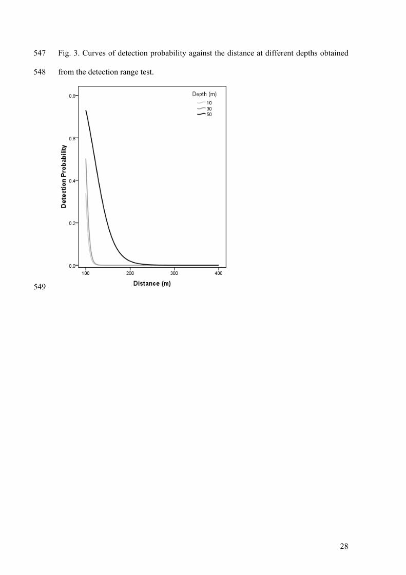
fitted using the lme4 library from the R data analysis software package (http://www.r-196
project.org/). A p-value of 0.05 was chosen a priori as the critical level for a rejection of 197
the null hypothesis. 198
The number of detections and the number of egg clutches corresponding to different 199
bathymetric depth intervals were compared using boxplots. The number of intervals 200
considered and their limits were selected to ensure that all of the intervals included a 201
large enough number of receivers. The squid tracks were also plotted; the maps were 202
produced using R package and improved using ArcGIS. 203

10
RESULTS 204
Detections 205
The results of the preliminary experiment aimed to explore the effects of depth and 206
distance to receiver showed significant differences of the probability detection among 207
depths (the probability increase with depth; GLM p < 0.001, Fig. 3). This result was 208
similar to those reported by Claisse et al. (2011). However, the distance at which 209
probability of detection is 0.5 was similar, especially when comparing the results 210
obtained at 10 and 30 m depth (97 m and 100 m; the same figure for 50 m depth is 120 211
m; Fig. 3). This result strongly support that in spite of the existence of some depth 212
effects, the detection probability is virtually the same at low and intermediate depth. 213
Additionally, in the view of these results, the simultaneous reception of the same 214
acoustic signal by more than one receiver was highly improbable. 215
A total of 8,835 true detections from 15 squid, out of the 26 tagged squid, were 216
downloaded. The number of detections of each squid ranged between a minimum of 15 217
detections (squid 11) and a maximum of 2,378 for the squid 46 (Table 1). The total 218
period (TP, in days) over which a squid was detected, defined as the number of days 219
from the tagging day to the last day a squid was detected, ranged from 2 (squid 77) to 220
31 (squid 111). The mean TP (± SD) was 11.53 ± 7.73 d. The number of days that a 221
squid was detected (DD) varied from 1 (squid 11) to 13 (squid 111 and 46). The mean 222
DD (±SD) was 6.13 ± 3.88 d. The average number of receivers that detected the same 223
squid was 2.06 ± 0.88 and ranged from 1 (squid 110, 11, 77) to 4 (squid 112 and 47). 224
The specific data for the squid are detailed in Table 1. 225
226
Temporal pattern 227

11
A preliminary inspection of the time series of the number of detections per time unit 228
does not reveal any clear pattern. However, the definition of the two types of visit event, 229
detection peaks and detection clusters, demonstrates the existence of significant 230
differences between day and night (GLMM p < 0.001, Fig. 4). During the daytime, the 231
squid tended to remain undetected, and very few visit events took place. However, in 232
those cases, the detections tended to form a detection cluster. In some cases, a detection 233
cluster even lasted most of the day (see examples in Fig. 4). Conversely, such long 234
detection clusters of the same squid on the same receiver were nearly absent between 235
sunset and sunrise. During the nighttime, the visit events tended to be shorter (detection 236
peaks instead of detection clusters; see some examples in Fig. 4). Moreover, new 237
appearances, when a specific squid was detected by two different receivers within the 238
same day, took place more frequently during the nighttime (squid 112 and 47; see the 239
stars in Fig. 4). 240
241
Space use 242
The number of detections was higher between 25 and 30 m of depth (Fig. 5 & 6). The 243
existence of some effects of depth on detection probability make that this results must 244
be interpreted with some caution. However, some patterns clearly emerge and they seem 245
robust against the small effects of depth: All of the squid were detected whitin the 25-30 246
m depth range (see some examples of the squid tracks in Fig. 5). Almost all (99.9%) of 247
the detections during the ATE1 experiment were made at this depth range, although it is 248
important to note that 61% of the receivers were deployed at this depth range. Similarly, 249
most of the detections (5,935, 99.26%) corresponded to the 25-30 m depth interval 250
during ATE2. Squid 110, 11 and 77 were detected by only one receiver that was placed 251
at the depth range of 25-30 m. Most of the rest of the squid (80%) were also detected in 252

12
this depth range. Nearly half of the squid moved between two closely positioned 253
receivers, but in those cases, they remained within the 25-30 m depth area (53.33%; 254
e.g., squid 4 and 7 in the Fig. 5A). Longer travels were performed by squid 108-10 and 255
112. The squid 108-10 toured 22.85 km during the 22 d of tracking. In the same way, 256
the squid 112 traveled 22.2 km during the 14 d of tracking. These longer travels were 257
also monitored by receivers deployed in the 25-30-m depth range (Fig. 5B). 258
During ATE2, squid were also detected by both deeper (at 31-38 m of depth) and 259
shallow receivers (at 16-24 m of depth). However, the prevalence of detections outside 260
the 25-30 m range was very low (0.14% and 0.60% for deep and shallow receivers, 261
respectively). Squid 47, a male, exemplified such a pattern. It reached receiver 19 at 16 262
m of depth from receiver 15 at 27 m of depth during the night but left this shallow water 263
before sunrise, and it appeared again in deeper waters at sunset (receiver 4 at 37 m 264
depth; see the grey star in the Fig. 4 and the movement track in the Fig. 5 C). 265
No squid were detected by the receivers placed in shallower waters (0-15 m depth), in 266
spite of the fact that some of the squid were tagged and released there. For example, 267
squid 46, a female, was fished, tagged and released in shallower waters without being 268
detected by receivers deployed in this shallow area. However, this squid was detected 269
one day later at 25 m of depth, and it spent some days in that area. After that period, this 270
squid left that area at sunset to reach deeper waters at sunrise (receiver 2 at 35 m depth; 271
Fig. 5C). 272
In relation to the spatial distribution of the fishing effort, the recreational fishers and 273
part of the commercial fleet concentrated at sunset and in specific areas located between 274
20-35 m of depth. After sunset, the commercial fishers continued to fish at the same 275
fishing ground but using lights. While that, after sunset, the recreational fishers 276

13
continued to fish for some time by trolling and focusing almost all of their effort from 277
the shoreline to 10 m of depth, just at the illuminated strip near the city lights (Fig. 7). 278
The presence of egg clutches was recorded from shallower waters (1 egg clutch at 279
receiver 17, at 9 m of depth) to deeper waters (3 egg clutches at receiver 9, at 38 m of 280
depth) (Figs. 6 & 7). The number of egg clutches was small (0.25 ± 0.5; ATE2 only) on 281
the receivers placed in shallower waters (0-15 m). The receivers deployed at a depth 282
interval between 16 and 24 m had mean values of 0.67 ± 0.58 and 0.5 ± 0.71 egg 283
clutches per receiver for ATE1 and ATE2, respectively. All of the receivers that were 284
deployed between 25 and 30 m had at least one egg clutch. The mean number of egg 285
clutches per receiver was clearly higher between 25 and 30 m (2.18 ± 1.40 and 2.40 ± 286
0.55 for ATE1 and ATE2, respectively). Finally, the receivers that were placed at a depth 287
between 31 and 38 m (only deployed during ATE2) had 1.17 ± 1.17 egg clutches 288
attached to their structures (Figs. 6 & 7). 289

14
DISCUSSION 290
The present study provides the first description of the movement patterns of the 291
European squid L. vulgaris during inshore spawning aggregations. The conceptual 292
model of movement proposed here is characterized by two well-differentiated 293
movement states. The typical daytime movement is characterized by a reduced mobility 294
within a narrow area, hereafter referred as day-ground. The squid tend to remain for a 295
long time (most of the daytime of a specific day) at a specific day-ground. However, the 296
location of the day-ground may change between consecutive days. This location may be 297
randomly selected within a larger area. The larger area is delimited by the Palma Bay 298
grounds at 25-30 m of depth. The typical nighttime movement is characterized by 299
increased mobility, i.e., a specific squid would spend only a short time at any given 300
location, and will range over a wider area. Such a night-ground possibly covers most of 301
the Palma Bay. This diel pattern might be due to periodic daily shifts between 302
reproduction behavior during the day and feeding at night. The empirical evidence 303
supporting this conceptual model emerges from 1) the existence of day-night 304
differences in the detection pattern using acoustic tracking, 2) the spatiotemporal 305
distribution of the fishing effort and 3) the spatial distribution of egg clutches. 306
The strongest evidence is from the day-night differences in the detection pattern. Squid, 307
when detected during the daytime, tended to remain near the detection range of only one 308
receiver in a detection cluster, supporting the hypothesis that the day-ground size is 309
small. However, a specific squid was usually not detected in two consecutive days by 310
the same receiver, suggesting that the day-ground location may change every day. 311
Almost all of the daytime detection clusters occurred within the 25-30-m depth area of 312
Palma Bay. We propose that the squid may be reproducing during the daytime within a 313
well-defined area. Evidence supporting this specific hypothesis emerges from 1) the 314

15
spatial distribution of egg clutches in Palma Bay and 2) the fact that the same pattern 315
(i.e., daytime reproduction) has been repeatedly described for other cephalopods. 316
Concerning the spatial distribution of eggs, other studies suggest that even though egg 317
clutches of L. vulgaris have been observed at depths from 2 m to 35 m, the clutches 318
were more frequent between 20-30 m (Villa et al. 1997), very close to the 25-30-m 319
depth area reported here. Concerning the daytime reproduction pattern, previous studies 320
demonstrated that during the daytime, L. reynaudii remains at the spawning grounds 321
(Sauer et al. 1997, Downey et al. 2009), where it performs a wide range of reproduction 322
behaviors, such as fighting, guarding, sneaking, mating and egg laying (Hanlon et al. 323
2002). The same activity pattern has been proposed for the Southern Calamari Squid 324
(Sepioteuthis australis Quoy & Gaimard, 1832), which arrives at sunrise at the vicinity 325
of the spawning grounds and spawns there throughout the daytime (Pecl et al. 2006). 326
Similarly, loliginid squid also showed reproductive activity during the daytime (Sauer et 327
al. 1997, Jantzen & Havenhand 2003, Forsythe et al. 2004). A plausible and biologically 328
sound explanation is that reproductive behaviors in cephalopods are strongly mediated 329
by visual cues (Hanlon & Messenger 1996). Specifically, visually detectable body 330
patterning plays an important courtship role during reproduction (Hanlon et al. 1994, 331
Hanlon & Messenger 1996, Hanlon et al. 1999, Hanlon et al. 2002). In fact, 332
intraspecific signaling in squid is known to occur mainly during daylight hours (Hanlon 333
& Messenger 1996). 334
During the nighttime, the squid were more mobile. The main empirical evidence 335
supporting this statement is that the squid, when detected at night, tend to remain for a 336
short time near a specific receiver, creating detection peaks instead of detection clusters. 337
We propose that L. vulgaris may be feeding during the nighttime. Increased activity 338
linked to feeding at night (beginning at dusk) has been described in other squid 339

16
(O’Sullivan & Cullen 1983, Hanlon & Messenger 1996). Specifically, nocturnal 340
predation has been proposed from the results obtained during other acoustic tracking 341
experiments (Sauer et al. 1997, Stark et al. 2005, Downey et al. 2009). The stomach 342
contents of L. reynaudii squid caught on the spawning grounds at night have more food 343
than those caught during the daytime (Sauer & Lipiński 1991), supporting an increased 344
predation activity during the nighttime like other loliginids. 345
Additional support for the conceptual model proposed here emerges from the 346
spatiotemporal distribution of the recreational fishing effort. The spatial aggregation of 347
the fishing effort has been adduced as indirect evidence for the spatial distribution of 348
squid (Boyle & Rodhouse 2005, Pecl et al. 2006, Olyott et al. 2007). In our case, 349
recreational fishing effort using line jigging concentrates between 20-35 m of depth 350
during the sunset. We propose that recreational line jigging concentrates within this 351
very narrow spatiotemporal window because squid catchability is higher. This 352
hypothesis is founded on the following: 1) squid concentrate during the daytime at 25-353
30-m depth region to form spawning aggregations, and these aggregations probably 354
break down at sunset due to a shift from reproduction to a feeding state (Downey et al. 355
2009), 2) squid probably feed during the nighttime, thus showing an increased interest 356
for lures, 3) squid display a higher mobility during the nighttime, thus increasing the 357
probability of encountering a lure and 4) at sunset, there is still enough light that favors 358
the detection of the lures used in line jigging. Commercial (artisanal) fishers do not stop 359
line jigging after dusk because they can use lights. Recreational fishers may continue to 360
fish after dusk, but only by trolling. The trolling method in shallower waters (from 361
shore to 10 m of depth) is performed by most of the anglers after fishing by line jigging. 362
In accordance with our conceptual model, squid after dusk enlarge their space use from 363
the 25-30-m depth area to a wider area that includes the trolling grounds. This pattern is 364
17
exemplified by squid 47 (see Fig. 4 & 5C). We hypothesize that this squid would 365
remained at the 25-30 m area during daytime but would became vulnerable to line 366
jigging only at sunset. This squid would be also vulnerable to trolling after dusk, when 367
it was detected at 16 m of depth, close to the trolling zone. 368

18
Acknowledgements. We thank the biologists and friends involved in experimental 369
angling seasons, especially Dra. B. Morales-Nin (IMEDEA), M. Calvo-Manazza, M. 370
Vidal-Arriaga, J. Maimó and L. Aguiló. Also, we thank Albatros Marine Technologies 371
S.L. for the design of the tag pistol. This study was partly financed by the research 372
project CONFLICT (CGL2008-958) funded by the Spanish Ministry of Science and 373
Innovation and by the Acció Especial “Determinación de la movilidad y estructura 374
poblacional de la especie diana Loligo vulgaris: aplicación del marcaje acústico y 375
genética poblacional” of the DG Investigación, Desarrollo Tecnológico e Innovación, 376
Conselleria de Innovación, Interior y Justicia, CAIB. The first author M. Cabanellas-377
Reboredo received a PhD fellowship by Conselleria de Educación, Cultura y 378
Universidades (Balearic Island Government) and Fondo Social Europeo (ESF) to 379
conduct research in Ocean Tracking Network at Dalhousie University (Halifax, Nova 380
Scotia, Canada). In this sense, the first author would like to thank the support and 381
hospitality of all OTN staff, mainly of Ellen Walsh, Dr. Frederick Whoriskey and the 382
suggestions of the Dr. Dale Webber during his research in Canada. Likewise, we would 383
like to thank the support and suggestions of Dr. John Payne (University of Washington; 384
Pacific Ocean Shelf Tracking). This paper is dedicated to Mayte Ortiz-Maldonado.385
19
LITERATURE CITED 386
Aitken JP, O’Dor RK, Jackson GD (2005) The secret life of the giant cuttlefish Sepia 387
apama (Cephalopoda): behaviour and energetics in nature revealed through radio 388
acoustic positioning and telemetry (RAPT). J Exp Mar Biol Ecol 320:77–91 389
Alós J, March D, Palmer M, Grau A, Morales-Nin B (2011) Spatial and temporal 390
patterns in Serranus cabrilla habitat use in the NW Mediterranean revealed by 391
acoustic telemetry Mar Ecol Prog Ser 427: 173-186 392
Augustyn CJ, Roel BA (1998) Fisheries biology, stock assessment, and management of 393
the chokka squid (Loligo vulgaris reynaudii) in South African waters: an overview. 394
Cal Coop Ocean Fish 39:71–80 395
Bates DM, Maechler M (2010) lme4: Linear Mixed-394 Effects Models Using S4 395 396
Classes. R package version 0.999375-36/r1083. available at: http://R-Forge.R-397
project.org/projects/lme4/ 398
Boyle PR, Pierce GJ, Hastie LC (1995) Flexible reproductive strategies in the squid 399
Loligo forbesi. Mar Biol 121: 501-508 400
Boyle P, Rodhouse P (2005) Cephalopods: Ecology and Fisheries. Blackwell 401
Publishing, UK 402
Botsford LW, Brumbaugh DR, Grimes C, Kellner JB and others (2009) Connectivity, 403
sustainability, and yield: bridging the gap between conventional fisheries 404
management and marine protected areas. Rev Fish Biol Fish 19:69–95 405
Cabanellas-Reboredo M, Alós J, Palmer M, Grädel M, Morales-Nin B (2011) 406
Simulating the indirect handline jigging effects on the European squid Loligo 407
vulgaris in captivity. Fish Res 408
Claisse JT, Clark TB, Schumacher BD, McTee SA, Bushnell ME, Callan CK, Laidley 409
CW, Parrish JD (2011) Conventional tagging and acoustic telemetry of a small 410

20
surgeonfish, Zebrasoma flavescens, in a structurally complex coral reef environment. 411
Environ Biol Fish 91: 185-201 412
Downey N, Roberts MJ, Baird, D (2009) An investigation of the spawning behaviour of 413
the chokka squid Loligo reynaudii and the potential effects of temperature using 414
acoustic telemetry. ICES J Mar Sci 67: 231-243 415
Dunstan AJ, Ward PD, Marshall NJ (2011) Vertical Distribution and Migration Patterns 416
of Nautilus pompilius. PLoS ONE 6: e16311. doi:10.1371/journal.pone.0016311 417
Forsythe J, Kangas N, Hanlon RT (2004) Does the Californian market squid (Loligo 418
opalescens) spawn naturally during the day or at night? A note on the successful use 419
of ROVs to obtain basic fisheries biology data. Fish Bull 102: 389–392 420
Gilly WF, Markaida U, Baxter CH, Block BA, Boustany A, Zeidberg L, Reisenbichler 421
K, Robison B, Bazzino G, Salinas C (2006) Vertical and horizontal migrations by the 422
jumbo squid Dosidicus gigas revealed by electronic tagging. Mar Ecol Prog Ser 324: 423
1–17 424
Gonçalves JM, Poteiro FM, Cardingos F, Martins HR, Pham CK (2009) The Azorean 425
Loligo forbesi (Cephalopoda: Loliginidae) in captivity: transport, handling, 426
maintenance, tagging and survival. Mar Biodivers Rec 2, doi: 427
10.1017/S1755267209001250 428
González M, Sánchez P (2002) Cephalopod assemblages caught by trawling along the 429
Iberian Peninsula mediterranean coast. Sci Mar 66: 199-208 430
Guerra A (1992) Mollusca Cephalopoda. Fauna Ibérica, Vol. 1. Museo Nacional de 431
Ciencias Naturales, CSIC, Madrid 432
Guerra A, Sánchez P, Rocha F (1994) The Spanish fishery for Loligo: recent trends. Fish 433
Res 21: 217-230 434

21
Guerra A, Rocha F (1994) The life history of Loligo vulgaris and Loligo forbesi 435
(Cephalopoda: Loliginidae) in Galician waters (NW Spain). Fish Res 21: 43-69 436
Hanlon RT, Smale MJ, Sauer WHH (1994) An erhogram of body patterning behaviour 437
in the squid Loligo vulgaris reynaudii on spawning grounds in South Africa. 438
Biol Bull 187: 363-372 439
Hanlon RT, Messenger JB (1996) Cephalopod Behaviour. Cambridge University Press, 440
Cambridge 441
Hanlon RT (1998) Mating systems and sexual selection in the squid Loligo: how might 442
commercial fishing on spawning squids affect them? Cal Coop Ocean Fish 39: 92–443
100 444
Hanlon RT, Maxwell MR, Shashar N, Loew ER, Boyle KL (1999) An ethogram of 445
body patterning in the medically and commercially valuable squid Loligo pealei off 446
Cape Cod, Massachusetts. Biol Bull 197: 49-62 447
Hanlon RT, Smale MJ, Sauer WHH (2002) The mating system of the squid Loligo 448
vulgaris reynaudii (Cephalopoda, Mollusca) off South Africa: fighting, guarding, 449
sneaking, mating and egg laying behaviour. Bull Mar Sci 71: 331–345 450
Iwata Y, Ito K, Sakurai Y (2010) Is commercial harvesting of spawning aggregations 451
sustainable? The reproductive status of the squid Loligo bleekeri. Fish Res 102: 286-452
290 453
Jantzen TM, Havenhand JN (2003) Reproductive behaviour in the squid Sepioteuthis 454
australis from South Australia: interactions on the spawning grounds. Biol Bull 455
204: 305–317 456
March D, Palmer M, Alós J, Grau A, Cardona F (2010) Short term residence, home 457
range size and diel patterns of thepainted comber Serranus scriba in a temperate 458
marine reserve. Mar Ecol Prog Ser 400: 195–206 459
22
March D, Alós J, Grau A, Palmer M (2011) Short-term residence and movement 460
patterns of the annular seabream Diplodus annularis in a temperate marine 461
reserve. Estuar Coast Shelf S 92: 581-587 462
Morales-Nin B, Moranta J, García C, Tugores P, Grau AM, Riera F, Cerdà M (2005) 463
The recreational fishery off Majorca Island (western Mediterranean): some 464
implications for coastal resource management. ICES J Mar Sci 62: 727-739 465
Moreno A, Pereira JMF, Arvanitidis C, Robin JP, Koutsoubas D, Perales Raya C, 466
Cunha MM, Balguerias E, Denis V (2002) Biological variation of Loligo 467
vulgaris (Cephalopoda: Loliginidae) in the eastern Atlantic and Mediterranean. 468
Bull Mar Sci 71: 515–534 469
Moreno A, Azevedo M, Pereira J, Pierce GJ (2007) Growth strategies in the squid 470
Loligo vulgaris from Portuguese waters. Mar Biol Res 3: 49-59 471
Ngoile MAK (1987) Fishery biology of the squid Loligo forbesi (Cephalopoda: 472
Loliginidade) in Scottish waters. PhD thesis, University of Aberdeen, UK 473
O'Dor RK, Hoar JA, Webber DM, Carey FG, Tanaka S, Martins HR, Porteiro FM 474
(1994) Squid (Loligo forbesi) performance and metabolic rates in nature. Mar 475
Freshw Behav Phy 25: 163-177 476
O’Dor R (2002) Telemetered cephalopod energetics: swimming, soaring and blimping. 477
Integr Comp Biol 42: 1065–1070 478
Olyott LJH, Sauer WHH, Booth AJ (2007) Spatial patterns in the biology of the chokka 479
squid, Loligo reynaudii on the Agulhas Bank, South Africa. Rev Fish Biol Fisher 480
17: 159-172 481
O’Sullivan D, Cullen JM (1983) Food of the Squid Nototodares gouldi in Bass Strait. 482
Aust J Mar Freshw Res 34: 261–285 483

23
Payne J, O’Dor RK (2006) Comparing Squid Optimal Cost of Transport Speeds to 484
Actual Field Migrations: New Data From 40-g Loligo opalescens. In: Olsen RJ, 485
Young JW (eds) The Role of Squid in Open Ocean Ecosystems. GLOBEC 486
Report 24: 16-18 487
Pecl GT, Tracey SR, Semmens JM, Jackson GD (2006) Use of acoustic telemetry for 488
spatial management of southern calamary Sepioteuthis australis, a highly mobile 489
inshore squid species. Mar Ecol Prog Ser 328: 1-15 490
Postuma FA, Gasalla MA (2010) On the relationship between squid and the 491
environment: artisanal jigging for Loligo plei at São Sebastião Island (24ºS), 492
southeastern Brazil. ICES J Mar Sci 67: 1353–1362 493
Rasero M, Portella JM (1998) Relationships between mating and sexual maturation of 494
Loligo gahi females in Falkland waters. J Mar Biol Ass UK 78: 673-676 495
Sánchez P, Guerra A (1994) Bathymetric distribution and aspects of the life history of 496
Loligo vulgaris in the Catalan Sea (NW Mediterranean). Iberus 12: 1-12 497
Sauer WHH, Lipiński MR (1991) Food of squid Loligo vulgaris reynaudii 498
(Cephalopoda: Loliginidae) on their spawning grounds off the Eastern Cape, 499
South Africa. S Afr J Marine Sci 10: 193–201 500
Sauer WHH, Roberts MJ, Lipiński MR, Smale MJ, Hanlon RT, Webber DM, O’Dor R 501
(1997) Choreography of the squid’s ‘Nuptial Dance’. Biol Bull (Woods Hole) 502
192:203–207 503
Semmens JM, Pecl GT, Gillanders BM, Waluda CM, Shea EK, Jouffre D, Ichii T, 504
Zumholz K, Katugin ON, Leporati SC, Shaw PW (2007) Aproaches to resolving 505
cephalopod movement and migraton patterns. Rev Fish Biol Fisher 17: 401-423 506

24
Šifner SK, Vrgoc N (2004) Population structure, maturation and reproduction of the 507
Common squid, Loligo vulgaris, in the Central Adriatic Sea. Fish. Res. 69: 239-508
249 509
Stark KE, Jackson GD, Lyle JM (2005) Tracking arrow squid movements with an 510
automated acoustic telemetry system. Mar Ecol Prog Ser 299: 167–177 511
Tinbergen L, Verwey J (1945) The biology of Loligo vulgaris Lam. Translation 512
Services Fisheries Research Board of Canada, 2733: 35 513
Ulaş A, Aydin I (2011) The effects of jig color and lunar bright on coastal squid jigging. 514
Afr J Biotechnol 10: 1721-1726 515
Villa H, Quintela J, Coelho M, Icely J, Andrade J.P (1997) Phytoplankton biomass and 516
zooplankton abundance in South Portugal (Sagres) with a special reference to the 517
spawning of Loligo vulgaris. Sci Mar 61: 123-129 518
Worms J (1983) Loligo vulgaris. In: Boyle PR (ed) Cephalopod life cycles. Vol 1. 519
Academic Press, London, p 143-158 520
25
TABLES 521
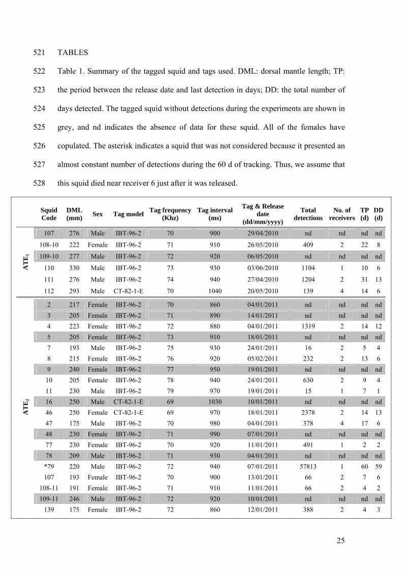
Table 1. Summary of the tagged squid and tags used. DML: dorsal mantle length; TP: 522
the period between the release date and last detection in days; DD: the total number of 523
days detected. The tagged squid without detections during the experiments are shown in 524
grey, and nd indicates the absence of data for these squid. All of the females have 525
copulated. The asterisk indicates a squid that was not considered because it presented an 526
almost constant number of detections during the 60 d of tracking. Thus, we assume that 527
this squid died near receiver 6 just after it was released. 528
Squid Code
DML (mm)
Sex Tag model Tag frequency
(Khz) Tag interval
(ms)
Tag & Release date
(dd/mm/yyyy)
Total detections
No. of receivers
TP(d)
DD(d)
107 276 Male IBT-96-2 70 900 29/04/2010 nd nd nd nd
108-10 222 Female IBT-96-2 71 910 26/05/2010 409 2 22 8
109-10 277 Male IBT-96-2 72 920 06/05/2010 nd nd nd nd
110 330 Male IBT-96-2 73 930 03/06/2010 1104 1 10 6
111 276 Male IBT-96-2 74 940 27/04/2010 1204 2 31 13
AT
E1
112 293 Male CT-82-1-E 70 1040 20/05/2010 139 4 14 6
2 217 Female IBT-96-2 70 860 04/01/2011 nd nd nd nd
3 205 Female IBT-96-2 71 890 14/01/2011 nd nd nd nd
4 223 Female IBT-96-2 72 880 04/01/2011 1319 2 14 12
5 205 Female IBT-96-2 73 910 18/01/2011 nd nd nd nd
7 193 Male IBT-96-2 75 930 24/01/2011 16 2 5 4
8 215 Female IBT-96-2 76 920 05/02/2011 232 2 13 6
9 240 Female IBT-96-2 77 950 19/01/2011 nd nd nd nd
10 205 Female IBT-96-2 78 940 24/01/2011 630 2 9 4
11 230 Male IBT-96-2 79 970 19/01/2011 15 1 7 1
16 250 Male CT-82-1-E 69 1030 10/01/2011 nd nd nd nd
46 250 Female CT-82-1-E 69 970 18/01/2011 2378 2 14 13
47 175 Male IBT-96-2 70 980 04/01/2011 378 4 17 6
48 230 Female IBT-96-2 71 990 07/01/2011 nd nd nd nd
77 230 Female IBT-96-2 70 920 11/01/2011 491 1 2 2
78 209 Male IBT-96-2 71 930 04/01/2011 nd nd nd nd
*79 220 Male IBT-96-2 72 940 07/01/2011 57813 1 60 59
107 193 Female IBT-96-2 70 900 13/01/2011 66 2 7 6
108-11 191 Female IBT-96-2 71 910 11/01/2011 66 2 4 2
109-11 246 Male IBT-96-2 72 920 10/01/2011 nd nd nd nd
AT
E2
139 175 Female IBT-96-2 72 860 12/01/2011 388 2 4 3

26
FIGURES 529
Fig. 1. Map of the receivers array deployed in 2010 (ATE1, panel A) and 2011 (ATE2, 530
panel B). The individual black points denote the receiver’s location. The damaged 531
receivers have been represented by a cross (receivers 9 and 11). The isobaths each 532
represent 10 m. 533
534

27
Fig. 2. Acoustic tracking logistics and methods. (A) Squid fished by line jigging. (B) 535
Squid sex and fertilization (females) determination. The image defined by the white 536
dashed line details the presence of a spermatophore in the ventral buccal membrane. (C) 537
Dorsal mantle length measurement to the nearest 5 mm. (D) Acoustic tags used in the 538
experiments with sterile hypodermic needles attached laterally to the tag. (E) An egg 539
clutch attached to a receiver rope. (F) Location of the acoustic transmitter. (G) Silicon 540
washers, which were pushed onto the ends of the hypodermic needles and slipped over 541
each needle. The metal cylinder was crimped using pliers to avoid the loss of 542
transmitter. (H) The tagged squid in an open seawater tank on the boat. The image 543
highlighted by the white dashed line shows the squid release in a tail-first direction 544
favoring the output of the air bubbles present in the mantle cavity. 545
546
28
Fig. 3. Curves of detection probability against the distance at different depths obtained 547
from the detection range test. 548
549

29
Fig. 4. Full time series of the detection numbers per hour of 4 tagged squid from ATE1 550
(108-10 and 112) and ATE2 (139 and 47). The vertical stripes represent day (white) and 551
night (grey). On the x-axis, each mark indicates the 00:00 hours of each day. When a 552
squid was detected by another receiver, the new receiver ID is indicated at the first 553
detection. The stars represent the new appearances, when a specific squid was detected 554
by two different receivers within the same day. 555
556

30
Fig. 5. Squid tracks assuming the minimum distance traveled (Pecl et al. 2006).

31
Fig. 6. Boxplot of the number of detections and egg clutches. The white boxes show the
data from ATE1, while the black boxes represent data from ATE2. Receivers were not
deployed in ATE1 within the depth range of 31-38 m. Outliers have been represented
with a star.

32
Fig. 7. Spatial distribution of the recreational fishing effort and egg clutch abundance in
Palma Bay. The isobaths each represent 10 m.