1

MFS605/EE605Systems for Factory Information and Control

Lecture 7 (Fall 2005)

Introductory Production Control and MRP

Larry Holloway

Dept. of Electrical and Computer Engineering and

UK Center for Manufacturing

2

• Where we’ve come from:

• Models of Manufacturing Systems:– Deterministic, Queuing, Simulation– Key ideas:

• Variation is undesirable:– If unbuffered, we sacrifice capacity– If buffered, we have more WIP, longer throughput time– M/M/1, M/M/c represents “practical worst-case”

variability (CV = 1)

• Some WIP useful for “buffering” stations, but…• More WIP Longer throughput time (Little’s law)

3

4

Key points of material so far:

• Relationship between WIP and time (Little’s law)

• Impact of variability

• Modeling for estimating time, WIP, performance– Deterministic– Stochastic/Queueing– Simulation models

Now… how do we manage the orders and inventory…?

5

Manufacturing Planning/Production Control

• Suppose we have a product designed

• Suppose we have a facility to produce it

Question: How do we operate the factory to produce the product?

--> Production Control

Production Control: coordination of resources to meet customer demands/orders.

(Resources mean: inventory, equipment, labor)

6

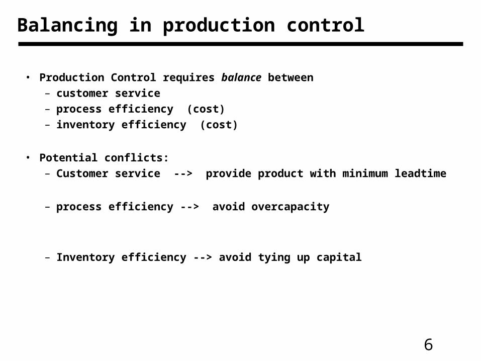
Balancing in production control

• Production Control requires balance between – customer service– process efficiency (cost)– inventory efficiency (cost)

• Potential conflicts:– Customer service --> provide product with minimum leadtime

– process efficiency --> avoid overcapacity

– Inventory efficiency --> avoid tying up capital

7

• inventory reduces cost through – fewer missed sales (if finished product available)– amortized setups– reduced order costs (administrative overhead)– reduced material cost through quantity discounts

• inventory contributes to cost through– cost of invested funds– cost of storage space– quality costs– coordination costs (tracking and transport of WIP)– Cost of poor responsiveness, obsolescence, decay

8

WIP

• WIP (Work in Process):– parts and products on the factory floor

• --> not in raw materials inventory• --> not in finished goods inventory

• WIP means money tied up since products not shippable

• (From Dilworth): Value of inventory in average manufacturing company is 1.61 months sales = 13.4% of annual sales– From 1988 to 1989, after tax profits of mfg. Companies averaged 5.4% sales– This means manufacturing company had 2.5 years of profits invested in

inventory

9

Breakdown of time spent by an average part in traditional metalworking batch manufacturing plant:

• Figures are from late 70’s, but still true in many companies today.

• One of the challenges in manufacturing is to reduce this non-value-added time.

Time on machine = 5%

Moving and waiting = 95%

30% cutting 70% loading, gauging, positioning

10

Production Control: the coordination of resources to meet customer demands/orders, balancing – customer service– process efficiency (cost)– inventory efficiency (cost)

• Example of complexity: modern jetliner.– How do we go about promising a delivery date?– How do we ensure necessary parts come together in a timely manner?

• Production control addresses these questions:– How much can we sell?– What parts do we need, and when?– What do we have in inventory?– What do we have to make, and when?– What is the lead time?– What processes are required?

11

• Process decoupling: separation of direct effects of different processes: – examples: job shop (high) vs. transfer line (low)– low decoupling --> higher inventory efficiency– high decoupling --> higher process efficiency

• Product Focus: How dedicated are facilities to a specific product.

Complex production control: many products,

lots of buffering

simpler production control: few products,

no buffering

Low Product Focus High

Pro

cess

Dec

ou

plin

gL

ow

H

igh

12

Production Control Classifications

Multiple-period inventory systems

• Methods for Independent Demands

– External demands (final products)

– Uncertainty

– Examples:

• Economic Order Quantity

• Fixed Quantity

• Fixed Interval

• Methods for Dependent Demands

– Demand depends directly on demand for higher level products.

– Examples:

• Push Systems (MRP)

• Pull Systems (JIT or lean manufacturing)

13

Independent Demand Inventory Methods

• Fixed Quantity Reorder

– reorder a fixed quantity when parts fall below reorder point

– good for parts with constant use rates

– “Two-bin” reorder useful for inexpensive parts

14

Independent Demand Inventory Methods

• Fixed Interval System

– at fixed time points, reorder to replenish up to fill line

– Useful when multiple part types from same supplier.

15

Minimum-maximum inventory systems (S,s)

• (S,s) system– S is maximum level– s is minimum level

• Inventory is reviewed at fixed intervals t• Order is placed only if inventory below minimum level s• Order is placed to refill up to level S

16

Economic Order Quantity

• Economic Order Quantity Model: allows determination of “optimal” order size or order period.• Assumes:

– demand is known and constant – setup cost and inventory costs are known

C=inventory carrying cost per unit per timeQ=batch sizeS=setup cost per batchD=Demand per unit time

17

EOQ

C=inventory carrying cost per unit per timeQ=batch size --> avg inventory level = Q/2S=setup cost per batchD=Demand per unit time

18

Economic Order Period

Optimal order period based on EOQ calculation

periodDemand

EOQperiodOptimal

/

19

Assumptions of EOQ

Assumptions of EOQ:

• Use rate is uniform and known (constant demand)

• Lead time is known in advance

• Cost of order is same regardless of amount ordered(item cost does not vary with order size (no quantity discounts))

• Cost of holding inventory is a linear function of # of items held (no economies of scale in holding)

• No backorders (all of order delivered at same time)

• No probability or uncertainty

• Setup and inventory costs assumed fixed

20

Summary so far…

• Production Control – coordinate resources (people, equipment, inventory) to meet customer demands/orders

• Independent Demand inventory methods…– Fixed Quantity Reorder – reorder fixed quantity whenever inventory

drops below trigger level– Fixed Interval System – reorder to refill at periodic interval– Minimum-Maximum (S,s) method: periodic ordering, order to refill to

level S, but only if inventory is below s.

– Economic Order Quantity: (EOQ): determine batch/order sizes based on inventory cost and setup cost

– Economic Order Period: Use EOQ to determine order period

21

ABC inventory classification

Classify and choose policy based on value:

A: items of highest expenditure (top 10-20%)– given greatest attention– may warrant constant record keeping– often fixed quantity reorder or frequent review interval

B: items of mid importance (next 20-30%)

C: items of lowest value– examples: bolts or screws– not worthwhile to track individually, don’t worry if some extra– just reorder on regular basis -- use simple methods

% of $ usage

% of items

22

ABC classification example (Dilworth)

• Note: keeping an extra month of “A” product #5294 is $8165 worth of inventory tied up. Keeping an extra month of “C” product #3521 is $474.25.

• Key idea of ABC: for A items, keeping extra inventory is costly, so it is worth careful tracking. For “C” items, keeping extra inventory is less costly, so use easy tracking methods to save on inventory tracking effort.

Item Annual Use in $ % of Sum Cum. %5294 97,982 44.42 44.425223 40,566 18.39 62.814395 17,028 7.72 70.538046 16,060 7.28 77.819555 15,602 7.07 84.886081 8,902 4.04 88.911837 8,222 3.73 92.643521 5,691 2.58 95.224321 4,488 2.03 97.269261 3,190 1.45 98.701293 2,127 0.96 99.672926 737 0.33 100.00

23

ABC continued…

• ABC useful for determining how to manage inventory based on its cost or value.

• Note that some items may be very critical but of low cost, and thus justify a higher rating than ABC gives them.

24

• DEPENDENT DEMAND INVENTORY MGT.

25

Production control for dependent demand items

• Dependent demand items:

• Example: Forklift:– each order requires 4 wheels, 4 tires, 1 seat, 1 steering

wheel, etc.

• Methods:– Push– Pull– OPT (drum-buffer-rope methods)

26

Raw materials Product

CUSTOMER

Push System• Customer orders and forecasts are fed into beginning of line

Manufacturing Facility

Forecasts

27

Supplierorder

Raw materials Product

CUSTOMER

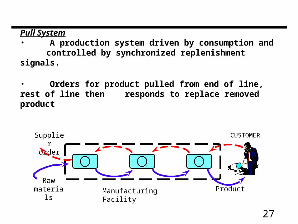
Pull System• A production system driven by consumption and controlled by synchronized replenishment signals.

• Orders for product pulled from end of line, rest of line then responds to replace removed product

Manufacturing Facility

28

Raw materials Product

CUSTOMER

Push System• Customer orders and forecasts are fed into beginning of line

Manufacturing Facility

Forecasts

29

Supplierorder

Raw materials Product

CUSTOMER

Pull System • Orders for product pulled from end of line, rest of line then responds to replace removed product

Manufacturing Facility

30

MRP / MRPII

MRP: Material Requirements PlanningMRPII: Manufacturing Resource Planning

• Typical Push system:– “explodes out” demand for final product into orders for raw materials and

subassemblies.

• began in 1960’s as computerized approach to materials planning (MRP)

• Later expanded (MRPII), which included:– master production scheduling– capacity requirements planning– purchasing– forecasting– financial modules

31

Background

• Popularity stems to the “MRP crusade” in 70’s by APICS (American Production and Inventory Control Society)

• Focus:– convince industry that MRP was integrated decision support

system for management of the total manufacturing business.

• Promoted by APICS, consultants, and computer industry

• Recently: MRP has come under fire:– oversold and poorly implemented– in practice, often leads to large WIP, large lead time

32

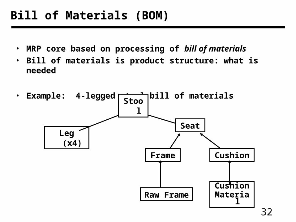
Bill of Materials (BOM)

• MRP core based on processing of bill of materials• Bill of materials is product structure: what is needed

• Example: 4-legged stool bill of materials

Frame

CushionMaterialRaw Frame

Leg (x4)

Cushion

Seat

Stool

33

• MRP Requires:– Master Production Plan

• (orders for finished products with due dates)– On-hand inventories

– Bill of materials

– Current Status of purchased and manufactured items

– Replenishment rules by item

• lead time• order quantity• safety stock

• scrap allowance, etc.

34

• MRP is calculating sizing and timing of net requirements for components/subassemblies

• Time is divided into “time buckets”

Given gross requirements for top level: • Projected Inventory = Previous Inventory + Scheduled Receipts

- Gross Requirements

• Determine net requirements based on projected inventory

• Shift back by lead time to determine when to order net reqmnts• Determine Gross Requirement for components by BOM, then repeat steps above

for components

35

Example:

• Bill of Materials for Stool A (4 legged) and Stool B (3 legged)

• Master Production Schedule:

• Other info: lead times (weeks) current inventory– Stool A: 2 10– Stool B: 2 30– Leg: 2 40 (20 more due week 3)– etc…..

36

MRP Example:

37

• Summary of basic method:– take final orders (gross reqmnts)

– determine net requirements (after inventory, sched recpts)

– from lead time, determine when to begin order

– from bill of materials, determine gross reqmnts of components

38

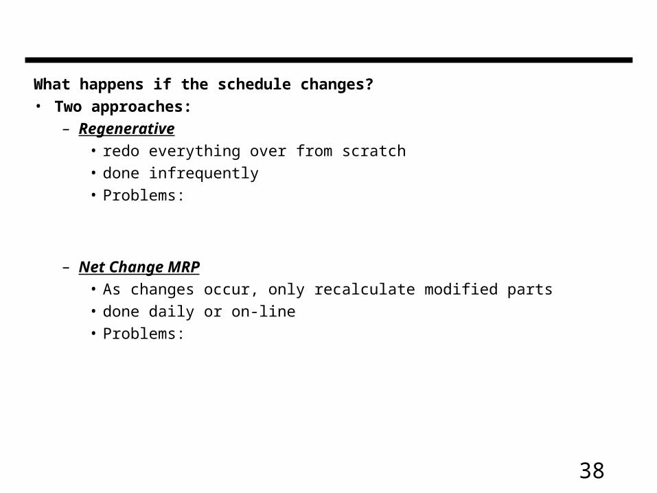
What happens if the schedule changes?• Two approaches:

– Regenerative• redo everything over from scratch• done infrequently• Problems:

– Net Change MRP• As changes occur, only recalculate modified parts• done daily or on-line• Problems:

39

Other issues of MRP

• Time buckets: – bucket is fixed time slot, and system has fixed # of buckets (planning

horizon)– typically buckets are 1 week

• note that there is no explicit indication as to whether event occurs at beginning or end of the bucket

• Safety Stocks:– excess quantities of inventory maintained to cover unexpected fluctuations

in supply or demand.– “Just-in-case” inventory

– 2 methods• always order stock to keep inventory above minimum• just hide safety stock from MRP system (don’t include in inventory)

40

Net change and regenerative are both “top-down” planning

“Bottom-up planning” is where human operator takes over– rush orders, special exceptions, scheduling

• Firm-planned orders: allows over-ride of MRP rules– override lot size or lead time

• Pegged Requirements: allows operator to see what final order is associated with given component orders (retrace the MRP steps)

41

MRP Review

• MRP: Materials Requirement Planning– computerized approach to translating orders for final

goods into orders for operations and raw materials– Key idea: Blow up bill of materials

• expand to subcomponents• factor in lead times• determine when operations and orders should be done

42

MRPII

• MRPII: Manufacturing Requirements Planning– built around MRP bill-of-materials processor– adds additional functionality:

• master production scheduling• capacity planning• financial modules• etc.

– Integrated set of manufacturing planning tools

43

Rough Cut Capacity Planning

• Blows out Bill of Resources similar to explosion of Bill of Materials for MRP

• Example: • Orders wk1 wk2 wk3

– Stool A: 100 150 120– Stool B: 180 180 180

Suppose we need 1 man hour per stool. (This is with setup time amortized)

Required hours: 280 330 300Available: 300 300 300Net: +20 -30

• Note: No real planning, just evaluation of requirements– Highlights resource constraints.

44

Positive aspects of MRP

• Better coordination of orders for dependent demand items…– May reduce WIP by ordering component products only as

needed for final product.– But…

• Production Planning: Helps determine peaks and valleys

• Purchasing and Finance: tells needs over the horizon.

• Sales: MRP helps sales by giving estimates of lead times…– But…

45

Issues with MRP

• MRP is useful for high-level planning.• Generally seen as a problem for low-level shop-floor control

• Issues: – buckets are too course for shop-floor control

– Lead times treated independent of demand or batch size

– Inflation of lead times or safety stock-- no method to see if these are too big, no method to encourage reduction

– Commonly gives large lead times and large WIP

– Assumes “Transfer quantity = order quantity”

46

Transfer Quantity vs. Order Quantity

• Example: 50 components in batch, 10 minutes per part.

47

Supplierorder

Raw materials Product

CUSTOMER

Pull System• A production system driven by actual consumption and

controlled by synchronized replenishment signals.

• Orders for product pulled from end of line, rest of line then responds to replace removed product

Manufacturing Facility

48

Just-in-time manufacturing

• Just-in-time manufacturing: “Lean Manufacturing”

• Key Concept: Continuous improvement to eliminate waste of all forms.

• Goals:– Minimum zero inventories– zero lead time– zero set up time– lot size of 1– zero defects– total elimination of waste

Is this realistic?

49

• We will just study the production control, but concept is much bigger. Affects:– transportation– supplier relations– quality– setup– employee responsibilities– …all aspects of organization…

50

• Background:– Toyota -- postwar Japan– Taichi Ohno: Chief production engineer.

– Not really noticed by US until 1970’s

Why so slow for West to notice or catch on?

51

JIT/Lean

• JIT/Lean is holistic approach– keep tackling all parts of system

• different aspects affect each other– example: lot sizing and setup time

– keep striving for continuous improvement

52

Conventional Mfg.

• Why did it take so long for US mfg. To understand?

Possible ideas: