1

1. Maximum likelihood method (ML)

1.1 Likelihood function

Problem:

While the distribution and thus the probability or density function f(y; θ) of a

random variable y (e.g. Bernoulli distribution, Poisson distribution, normal dis-

tribution) is known, some parameters of this distribution that are summarized in

the vector θ = (θ1, θ2,…, θm)‘ are unknown and have to be estimated

→ For this purpose a random sample y1,…, yn of n observations is drawn from

the corresponding distribution where fi(yi; θ) is the probability or density

function of yi for observation i

Due to the independence of the yi, the joint probability function (for discrete

random variables) or density function (for continuous random variables) of the

y1,…, yn is the product of the individual probability or density functions:

If this function is not considered as a function of the random sample y1,…, yn

given the parameters in θ, but as a function of θ for a given random sample

y1,…, yn, it can be interpreted as a likelihood function:

n

1 n 1 1 n n i i

i=1

f (y ,..., y ; θ) = f (y ; θ) f (y ; θ) = f (y ; θ)

2

It should be noted that the likelihood function as well as all following derived

functions are random variables (or random vectors or random matrixes) before

the drawing of a random sample.

The idea of the maximum likelihood method is to find the value θ of θ that ma-

ximizes the likelihood function on the basis of the random sample y1,…, yn.

However, the maximization procedure is generally not based on the likelihood

function, but on the log-likelihood function, i.e. the following natural logarithm:

The maximization of logL(θ) leads to the same estimator θ as the maximiza-

tion of L(θ). Advantages of the use of the log-likelihood function:

• The use of logL(θ) avoids extremely small values in the case of discrete ran-

dom variables (due to the multiplication of probabilities and thus values that

are smaller than one) and extremely high values in the case of continuous

random variables (if values that are higher than one in the density functions

are multiplied)

• Generally, the maximization process to receive θ is much simpler for the log-

likelihood function than for the likelihood function

n

i i

i=1

L(θ) = f (y ; θ)

n

1 1 n n i i

i=1

logL(θ) = logf (y ; θ) + + logf (y ; θ) = logf (y ; θ)

3

---------------------------------------------------------------------------------------------------------

Example: Bernoulli distribution

The probability function of a Bernoulli distributed random variable y with para-

meter p is:

If a random sample y1,…, yn of n observations is drawn from a Bernoulli distri-

bution with parameter p, this leads to the following likelihood and log-likelihood

functions:

---------------------------------------------------------------------------------------------------------

1-y y

1 - p for y = 0

f y; p = p for y = 1

0 else

or

f y; p = (1-p) p for y = 0, 1

1 1 n n i i

n1-y y 1-y y 1-y y

i=1

L(θ) = L(p) = (1-p) p (1-p) p = (1-p) p

1 1 n n

n

i i

i=1

logL(θ) = logL(p) = (1-y )log(1-p) + y log p + + (1-y )log(1-p) + y log p

= (1-y )log(1-p) + y log p

4

Maximization approach:

The ML estimator θ is therefore the value of θ that maximizes the log-likelihood

function.

The first derivative of the log-likelihood function is called score (function):

n'

1 2 m i iθ θ

i=1

ˆ ˆ ˆ ˆθ = θ , θ ,…, θ = arg max logL θ = arg max logf (y ; θ)

n

i i

i=1

1

1 n

i i

i=1

2

2

n

i im

i=1

m

logf (y ; θ)

logL(θ)θ

θ

logL(θ) logf (y ; θ)logL(θ)

θs(θ) = = = θθ

logL(θ)

logf (y ; θ)θ

θ

5

Due to the sum of the terms in the log-likelihood function, the score is also an

additive function:

Expectation of the score at the true, but unknown parameter vector θ:

The second derivative of the log-likelihood function is called Hessian matrix:

n ni i

i

i=1 i=1

logf (y ; θ)s(θ) = s (θ)

θ

E s(θ) = 0

2 2 2

2

1 2 1 m1

2 2 2

22

2 1 2 m2

2 2 2

2

m 1 m 2 m

logL(θ) logL(θ) logL(θ)

θ θ θ θθ

logL(θ) logL(θ) logL(θ)logL(θ)

θ θ θ θH(θ) = = θθ θ

logL(θ) logL(θ) logL(θ)

θ θ θ θ θ

6

Due to the sum of the terms in the log-likelihood function, the Hessian matrix is

also an additive function:

A necessary condition for the ML estimator θ is that the score for this value of θ

is zero:

As a consequence, the maximization process of the ML estimator can be char-

acterized as follows:

Additional necessary and sufficient condition for the ML estimator θ :

The Hessian matrix for this value of θ must be negative definite (if there is a so-

lution at an inner point of the parameter space). The maximum can be local or

global. In many simple cases the log-likelihood function is globally concave so

that the solution of the first order condition leads to a unique and global maxi-

mum of the log-likelihood function.

n ni i

iθ

i=1 i=1

logf (y ; θ)θ̂ = argsolves s(θ) = s (θ) = 0

θ

n

iˆ i=1θ

logL(θ) ˆ ˆ = s(θ) = s (θ) 0θ

2n ni i

i

i=1 i=1

logf (y θ)

θ θ

; H(θ) = H (θ)

7

---------------------------------------------------------------------------------------------------------

Example: Bernoulli distribution

If a random sample y1,…, yn of n observations is drawn from a Bernoulli distri-

bution with parameter p, this leads to the following score:

From the maximization of the log-likelihood function and thus equalizing the

score with zero, it follows that the ML estimator of the probability p is equal to

the sample mean, i.e. the proportion of ones in the sample:

The following second derivative of the log-likelihood function and thus the Hes-

sian matrix (i.e. scalar) is generally negative for all possible samples y1,…, yn:

---------------------------------------------------------------------------------------------------------

n ni i

i

i=1 i=1

n n ni i i i i

i=1 i=1 i=1

(1-y )log(1-p) + y log plogL(p) = s(p) = s (p)

p p

1-y y y (1-p) - p(1-y ) y -p - + = =

1-p p p(1-p) p(1-p)

n

i

i=1

1p̂ = y = y

n

ni i

2 2i=1

y 1-yH(p) = - -

p (1-p)

8

All previous concepts for unconditional models with a random variable y can be

simply transferred to conditional models and thus microeconometric models

with a dependent variable y and k explanatory variables which are summarized

in the vector x = (x1,…, xk)‘ in the following. xi = (xi1,…, xik)‘ is therefore the vec-

tor of explanatory variables for observation i.

With the conditional probability or density function f(y; x, θ) of y and a random

sample (yi, xi) (i = 1,…, n) it follows for the conditional joint probability or density

function:

It follows for the log-likelihood function, the score, the Hessian matrix, and the

maximization approach:

n

1 n 1 n 1 1 1 n n n i i i

i=1

f (y ,..., y ; x ,..., x , θ) = f (y ; x , θ) f (y ; x , θ) = f (y ; x , θ)

n

i i iθ

i=1

θ̂ = arg max logf (y ; x , θ)

n

i i i

i=1

logL(θ) = logf (y ; x , θ)n

i i i

i=1

logf (y ; x , θ)s(θ) =

θ

2ni i i

i=1

logf (y θ)

θ θ

; x , H(θ) =

9

---------------------------------------------------------------------------------------------------------

Example 1: General classical linear regression models (I)

With xi = (xi1,…, xik)‘ as the vector of k explanatory variables (including a con-

stant) and the corresponding k-dimensional parameter vector β = (β1,…, βk)‘,

the linear regression model has the following form (for i = 1,…, n):

Due to the normality assumption for the error term εi it follows:

Density function of yi:

Log-likelihood function on the basis of a random sample of n pairs of observa-

tions (yi, xi) (i = 1,…, n):

---------------------------------------------------------------------------------------------------------

i i iy = β'x + ε

2

i i iy |x ~ N(β'x ; σ )

2 211

2 2i i i i22i i i

1 1 y - β'x 1 y - β'xf (y ; x , β, σ ) = exp - = 2π σ exp -

2 σ 2 σσ 2π

2n2 2 i i

i=1

n2 2

i i2i=1

1 1 1 y - β'xlogL(θ) = logL(β, σ ) = - log(2π) - log(σ ) -

2 2 2 σ

n n 1 = - log(2π) - log(σ ) - (y - β'x )

2 2 2σ

10

---------------------------------------------------------------------------------------------------------

Example 1: General classical linear regression models (II)

First order conditions for maximizing the log-likelihood function:

The partial derivative of logL(β, σ2) with respect to β is a k-dimensional vector.

It follows for the ML estimator of β:

The inverse of the (k×k) matrix exists if there is no exact linear relationship bet-

ween the explanatory variables. The ML estimator β is therefore identical to the

corresponding OLS estimator (in the classical linear regression model). The

reason for this is that the first order conditions for optimizing the respective ob-

jective functions are identical.

---------------------------------------------------------------------------------------------------------

2 n

i i i2i=1

2 n2

i i2 2 4i=1

logL(β, σ ) 1 = x (y - β'x ) = 0

β σ

logL(β, σ ) n 1 = - + (y - β'x ) = 0

σ 2σ 2σ

-1n n

i i i i

i=1 i=1

β̂ = x x ' x y

(k×k) (k×1)

11

---------------------------------------------------------------------------------------------------------

Example 1: General classical linear regression models (III)

In contrast, the following ML estimator of σ2 differs from the familiar OLS esti-

mator of the variance of the error term:

While this estimator is biased, it is consistent and asymptotically efficient (see

below).

The following Hessian matrix is generally negative definite so that these para-

meter values actually refer to the maximum of the log-likelihood function:

---------------------------------------------------------------------------------------------------------

n2 2

i

i=1

1ˆσ̂ = ε

n

n n

i i i i i2 4i=1 i=12

n n2

i i i i i4 4 6i=1 i=1

1 1- x x ' - x (y - β'x )

σ σH(β, σ ) =

1 n 1- (y - β'x )x ' - (y - β'x )

σ 2σ σ

12

---------------------------------------------------------------------------------------------------------

Example 2: Determinants of (the logarithm of) wages (I)

By using a classical linear regression model, the effect of the years of educa-

tion (educ), the years of labor market experience (exper), and the years with

the current employer (tenure) on the logarithm of hourly wage (logwage) is exa-

mined on the basis of n = 526 workers:

However, instead of an OLS estimation, we now consider an ML estimation of

the parameters. Such estimations can be conducted with the STATA command

(“ml model”) including the lf method, which assumes the independence of the

observations and uses numerical first and second derivatives of the log-likeli-

hood function. For different ML estimations with STATA, separate programs

have to be written which specify the log-likelihood functions.

Components of the program (“linearregression”, which is an arbitrary term):

• Three arguments: Logarithm of individual density function (“loglikelihood”),

β‘xi (“betaxi“), σ2 (“sigmasquared”)

• Logarithm of density function of yi (i.e. individual log-likelihood function):

---------------------------------------------------------------------------------------------------------

0 1 2 3logwage = β + β educ + β exper + β tenure + ε

2 2 2

i i i i i2

1 1 1logf (y ; x , β, σ ) = - log(2π) - log(σ ) - (y - β'x )

2 2 2σ

13

---------------------------------------------------------------------------------------------------------

Example 2: Determinants of (the logarithm of) wages (II)

The STATA command “ml model lf” includes the definition of the dependent and

explanatory variables and the STATA command “ml maximize” finally presents

the estimation results. This ML estimation leads to the following results:

program linearregression

args loglikelihood betaxi sigmasquared

quietly replace `loglikelihood' = (-1/2)*ln(2*_pi) - (1/2)*ln(`sigmasquared')-

(1/(2*`sigmasquared'))*($ML_y1-`betaxi')^2

end

ml model lf linearregression (Betas: logwage = educ exper tenure) (Variance:)

ml maximize

Number of obs = 526

Wald chi2(3) = 243.02

Log likelihood = -313.54779 Prob > chi2 = 0.0000

------------------------------------------------------------------------------

logwage | Coef. Std. Err. z P>|z| [95% Conf. Interval]

-------------+----------------------------------------------------------------

Betas |

educ | .092029 .007302 12.60 0.000 .0777173 .1063406

exper | .0041211 .0017167 2.40 0.016 .0007564 .0074858

tenure | .0220672 .0030819 7.16 0.000 .0160269 .0281076

_cons | .2843595 .1037935 2.74 0.006 .080928 .4877909

-------------+----------------------------------------------------------------

Variance |

_cons | .1928813 .0118936 16.22 0.000 .1695704 .2161923

------------------------------------------------------------------------------

---------------------------------------------------------------------------------------------------------

14

---------------------------------------------------------------------------------------------------------

Example 2: Determinants of (the logarithm of) wages (III)

In contrast, the OLS estimation with STATA leads to the following results (see

also chapter 0):

reg logwage educ exper tenure

Source | SS df MS Number of obs = 526

-------------+------------------------------ F( 3, 522) = 80.39

Model | 46.8741806 3 15.6247269 Prob > F = 0.0000

Residual | 101.455582 522 .194359353 R-squared = 0.3160

-------------+------------------------------ Adj R-squared = 0.3121

Total | 148.329763 525 .282532881 Root MSE = .44086

------------------------------------------------------------------------------

logwage | Coef. Std. Err. t P>|t| [95% Conf. Interval]

-------------+----------------------------------------------------------------

educ | .092029 .0073299 12.56 0.000 .0776292 .1064288

exper | .0041211 .0017233 2.39 0.017 .0007357 .0075065

tenure | .0220672 .0030936 7.13 0.000 .0159897 .0281448

_cons | .2843595 .1041904 2.73 0.007 .0796755 .4890435

------------------------------------------------------------------------------

The ML and OLS estimates of the parameters in β are therefore completely

identical (the estimation of the variance σ2 is no component of the OLS estima-

tion). Only the estimated standard deviations of the estimated parameters are

slightly different due to imprecisions in the maximization process of the log-like-

lihood function.

---------------------------------------------------------------------------------------------------------

15

1.2 Properties of the ML estimator

Finite sample properties of the ML estimator θ of θ:

• θ is often a biased estimator of θ (e.g. the expectation of σ 2 is not equal to

σ2 in the classical linear regression model, whereas β is unbiased in this

case which is, however, an exception)

• θ is generally not normally distributed (the normal distribution of β in the

classical linear regression model is again an exception)

• The generally unknown small sample properties of ML estimators can be

examined by Monte Carlo simulations for specific (microeconometric) mo-

dels and specific parameter values

Asymptotic properties of the ML estimator θ of θ (under several regularity con-

ditions and if the underlying model is correctly specified):

• Consistency, i.e. P(|θ – θ| > ξ) converges (for ξ > 0) to zero for n → ∞ or

plim(θ ) = θ. This means that the asymptotic distribution of θ is centered at θ

and its variance goes to zero. An alternative notation for the consistency is:

• Asymptotic normality

• Asymptotic efficiency

p

θ̂ θ

16

The asymptotic normality does not directly refer to the ML estimator θ , but to

n(θ -θ):

This means that n(θ -θ) converges in distribution to the normal distribution, i.e.

is asymptotically normally distributed with an expectation vector zero and the

variance covariance matrix I(θ)-1. The matrix I(θ) is called information matrix

and has the following form:

The inverse of the information matrix is the Cramer Rao lower bound which im-

plies that the difference between this matrix and the corresponding variance

covariance matrix for any other consistent estimator of θ, for which n(θ -θ) is

asymptotically normally distributed, is negative definite. Since n(θ -θ) reaches

this lower bound, the ML estimator is asymptotically efficient.

Information matrix equality at the true, but unknown parameter vector θ:

This equality means that the variance covariance matrix of the score for obser-

vation i is identical to the negative expectation of the Hessian matrix for i and

thus the information matrix.

a d

-1 -1ˆ ˆn(θ - θ) ~ N 0; I(θ) or n (θ - θ) N 0; I(θ)

i i i iI(θ) = -E H (θ) = E s (θ)s (θ)' = Var s (θ)

2

i ii

logf (y ;θ)I(θ) = -E = -E H (θ)

θ θ'

17

From the asymptotic normality of n(θ -θ) it follows that the ML estimator θ is

approximately normally distributed for large but finite samples of n observa-

tions:

The variance covariance matrix of θ thus has the following form:

However, the information matrix (and this symmetric and positive definite vari-

ance covariance matrix) is unknown in practice since it depends on the un-

known θ and thus has to be (consistently) estimated, e.g. for statistical tests

and the construction of confidence intervals. Var(θ ) can be estimated by inclu-

ding the ML estimator θ instead of the true parameter vector:

However, it is often not possible to obtain an exact expression for the expecta-

tion.

appr

-1θ̂ ~ N θ; nI(θ)

1 1 2 1 m

-1 -12 1 2 2 m

i

m 1 m 2 m

ˆ ˆ ˆ ˆ ˆVar(θ ) Cov(θ ,θ ) Cov(θ ,θ )

ˆ ˆ ˆ ˆ ˆCov(θ ,θ ) Var(θ ) Cov(θ ,θ )ˆVar(θ) = = nI θ = -E nH θ

ˆ ˆ ˆ ˆ ˆCov(θ ,θ ) Cov(θ ,θ ) Var(θ )

-1

iˆ ˆˆVar(θ) = -E nH (θ)

18

In practice the following two estimators for the variance covariance matrix (in-

cluding consistent estimators of the information matrix) are commonly used:

The first estimator exclusively incorporates the Hessian matrix at the ML esti-

mator for the observations, whereas the second approach exclusively includes

the score at the ML estimator and is called the outer product of the gradient.

A third approach follows from the quasi maximum likelihood theory and in-

cludes a robust estimator of the information matrix that can even be consistent

with respect to the true information matrix if the underlying model is misspeci-

fied. It includes both the Hessian matrix and the score at the ML estimator:

All three estimators of the information matrix are asymptotically equivalent, but

can be very different in small samples.

-1 -1n n-1

1 1 i i

i=1 i=1

-1 -1n n-1

2 2 i i i i

i=1 i=1

1ˆ ˆ ˆ ˆˆˆVar(θ) = nI(θ) = - n H (θ) = - H (θ)n

1ˆ ˆ ˆ ˆ ˆ ˆˆˆVar(θ) = nI(θ) = n s (θ)s (θ)' = s (θ)s (θ)'n

-1 -1n n n-1

3 3 i i i i

i=1 i=1 i=1

-1

1 2 1

ˆ ˆ ˆ ˆ ˆ ˆˆˆVar(θ) = nI(θ) = H (θ) s (θ)s (θ)' H (θ)

ˆ ˆ ˆˆ ˆ ˆ = Var(θ) Var(θ) Var(θ)

19

Invariance principle:

The ML estimator of any function h(θ) of θ is the function h(θ ) of the ML estima-

tor θ . Since it is an ML estimator, it is consistent, but usually not unbiased.

Delta method:

The estimator of the variance covariance matrix of the ML estimator h(θ ) of the

function h(θ) is a quadratic form of the derivatives of h(θ) and an estimator of

the variance covariance matrix of θ .

Problem of maximization of the log-likelihood function:

A very efficient way to find the ML estimator θ in the maximization process is

the analytical optimization by equaling the score to zero and solving for the ma-

ximizing parameters. However, this approach requires a closed form solution of

the first order condition for maximizing the log-likelihood function. Indeed, in

many cases it is not available due to the non-linearity of the log-likelihood func-

tion so that iterative numerical maximization algorithms have to be applied

such as the Newton Raphson algorithm or the BHHH algorithm.

'

ˆ ˆθ θ

h(θ) h(θ)ˆ ˆˆ ˆVar h(θ) = Var(θ)θ θ

20

1.3 Statistical testing

Problem:

The ML estimation of (microeconometric) models leads to a corresponding

point estimate, but does not account for the sampling variability which is the

basis for the construction of confidence intervals and for statistical tests

Testable hypotheses refer to restrictions on the parameter space. The following

general null and alternative hypotheses are based on q such restrictions:

In the simplest case, the dimension of the function c(θ) is q = 1 and c(θ) refers

to specific values of one parameter θl of the vector θ which leads to the follow-

ing null hypothesis (with an arbitrary constant a):

On the basis of the ML estimation of (microeconometric) models, these null hy-

potheses can be statistically tested with the Wald test, the likelihood ratio test,

or the score test which are asymptotically equivalent.

1

0

q

1

c (θ) = 0

H : c(θ) = 0

c (θ) = 0

H : c(θ) 0

0 lH : θ = a

21

Wald test procedure:

This test is based on the unrestricted ML estimator θ . Under the null hypothesis

H0: c(θ) = 0 it follows that c(θ ) converges stochastically to zero since it is a con-

sistent estimator of c(θ). Therefore, the alternative hypothesis implies that c(θ )

strongly differs from the null vector.

Wald test statistic:

I (θ ) is a consistent estimator of the information matrix and can e.g. be estima-

ted on the basis of the three versions as discussed above. If H0: c(θ) = 0 is

true, it follows that the Wald test statistic is asymptotically χ2 distributed with q

degrees of freedom, i.e.:

Thus, the null hypothesis is (for a large sample size n) rejected in favor of the

alternative hypothesis at the significance level α if:

-1ˆ ˆc(θ) c(θ)'ˆ ˆ ˆˆWT = nc(θ)' I(θ) c(θ)

θ' θ

d2

qWT χ

2

q;1-αWT > χ

22

In the case of the specific simple null hypothesis H0: θl = a it follows that the

corresponding Wald test statistic is asymptotically χ2 distributed with one de-

gree of freedom. Therefore, it follows the simplest and most important version

of a Wald test statistic, namely the z statistic (or t statistic), which is asymptoti-

cally standard normally distributed:

The estimated variance of θ l is the l-th diagonal element of the estimated vari-

ance covariance matrix of θ (e.g. on the basis of the three versions as dis-

cussed above). The null hypothesis is thus (for a large sample size n) rejected

at the significance level α if:

Restricted ML estimation:

An ML estimator θ r is called restricted ML estimator if the underlying ML esti-

mation is based on specific restrictions for the unknown parameters. In the sim-

plest case the restriction refers to specific values for unknown parameters. For

example, if θ = (α, β)‘, a possible restriction is α = 1 so that the restricted ML

estimator is θ r = (1, β r)‘, whereas the unrestricted ML estimator is θ u = (α u, β u)‘.

dl

l

θ̂ - aWT = z = N(0; 1)

ˆˆVar(θ )

1-α/2z > z

23

Likelihood ratio test procedure:

This test is based on both the unrestricted ML estimator θ u and the restricted

ML estimator θ r. In the following, the value of the log-likelihood function at the

restricted ML estimator is denoted by logL(θ r) and the value of the log-likeli-

hood function at the unrestricted ML estimator is denoted by logL(θ u), where

logL(θ r) ≤ logL(θ u). The null hypothesis H0: c(θ) = 0 implies that these values

are very similar, whereas the alternative hypothesis implies that the values of

the restricted and unrestricted log-likelihood functions are strongly different.

Likelihood ratio test statistic:

If H0: c(θ) = 0 is true, it follows that the likelihood ratio test statistic is asymptoti-

cally χ2 distributed with q degrees of freedom, i.e.:

Thus, the null hypothesis is (for a large sample size n) rejected in favor of the

alternative hypothesis at the significance level α if:

The main advantage of this test is that it is easy to perform. The practical dis-

advantage is that two models have to be estimated separately.

u rˆ ˆLRT = 2 logL(θ ) - logL(θ )

d2

qLRT χ

2

q;1-αLRT > χ

24

Score test procedure:

This test is only based on the restricted ML estimator θ r. It is further based on

the property that the expectation of the score at the true, but unknown parame-

ter vector θ is zero and that the score (i.e. the first derivative of the log-likeli-

hood function) at the unrestricted ML estimator θ u is zero (necessary condition

for the ML estimator). The score test therefore considers the difference bet-

ween the score at the restricted ML estimator θ r and the null vector. The null

hypothesis H0: c(θ) = 0 implies that these values are very similar, whereas the

alternative hypothesis implies that the difference is large.

Score test statistic:

Under H0: c(θ) = 0, I (θ r) is a consistent estimator of the information matrix and

can e.g. be estimated on the basis of the three versions as discussed above. If

H0 is true, it follows that the score test statistic is asymptotically χ2 distributed

with q degrees of freedom, i.e.:

Thus, the null hypothesis is (for a large sample size n) rejected in favor of the

alternative hypothesis at the significance level α if:

d2

qST χ

2

q;1-αST > χ

-1r rr

ˆ ˆ1 logL(θ ) logL(θ )ˆˆST = I(θ )n θ' θ

25

---------------------------------------------------------------------------------------------------------

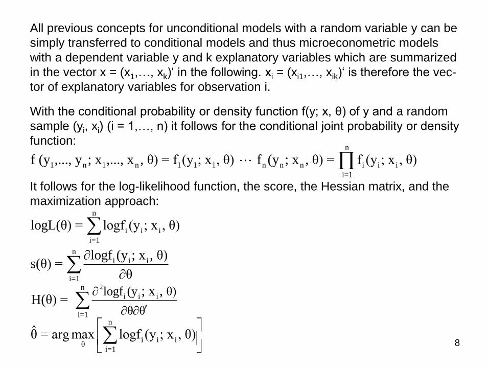
Example: Determinants of (the logarithm of) wages (I)

Based on the discussed ML estimation of the classical linear regression model,

which considers the effect of the years of education (educ), the years of labor

market experience (exper), and the years with the current employer (tenure) on

the logarithm of hourly wage (logwage), the null hypothesis that neither educ

nor exper has any effect on logwage, i.e. that the two parameters of educ and

exper are both zero, is tested. The command for the Wald test in STATA is:

test educ=exper=0

( 1) [Betas]educ - [Betas]exper = 0

( 2) [Betas]educ = 0

chi2( 2) = 161.52

Prob > chi2 = 0.0000

The application of the likelihood ratio test requires both the unrestricted and

restricted ML estimation. After the unrestricted ML estimation the following

STATA command for saving the estimation results is necessary (the choice of

the name “unrestricted” is arbitrary):

estimates store unrestricted

After the restricted ML estimation a corresponding STATA command for saving

the respective estimation results is necessary (the choice of the name “restric-

ted” is again arbitrary).

---------------------------------------------------------------------------------------------------------

26

---------------------------------------------------------------------------------------------------------

Example: Determinants of (the logarithm of) wages (II)

ml model lf linearregression (Betas: logwage = tenure) (Variance:)

ml maximize

Number of obs = 526

Wald chi2(1) = 62.35

Log likelihood = -383.97797 Prob > chi2 = 0.0000

------------------------------------------------------------------------------

logwage | Coef. Std. Err. z P>|z| [95% Conf. Interval]

-------------+----------------------------------------------------------------

Betas |

tenure | .0239514 .0030333 7.90 0.000 .0180063 .0298965

_cons | 1.501007 .0268149 55.98 0.000 1.448451 1.553563

-------------+----------------------------------------------------------------

Variance |

_cons | .2521113 .0155458 16.22 0.000 .221642 .2825806

------------------------------------------------------------------------------

estimates store restricted

Command for the likelihood ratio test in STATA:

lrtest unrestricted restricted

Likelihood-ratio test LR chi2(2) = 140.86

(Assumption: restricted nested in unrestricted) Prob > chi2 = 0.0000

Both the Wald test and the likelihood ratio test therefore lead to the rejection of

the null hypothesis at very low significance levels.

---------------------------------------------------------------------------------------------------------

27

Model selection:

The underlying hypotheses in the three tests imply two (microeconometric) mo-

dels that are nested, i.e. one model is a restricted version of the other model. If

two models are non-nested, a selection between them can be based on the

higher value of the log-likelihood function at the ML estimators. However, these

values depend on the number of parameters in the models so that this number

should be considered in a model selection. Two common approaches in this

respect are the Akaike information and Schwarz information criteria.

Goodness-of-fit:

In linear regression models, the coefficient of determination R2 is an appropri-

ate goodness-of-fit measure. However, in many microeconometric models this

measure is not available. Based on the value logL(θ u) of the log-likelihood func-

tion at the ML estimator of the full microeconometric model with all explanatory

variables (including a constant) and the value logL(θ r) at the restricted ML esti-

mator of the corresponding model that only includes the constant, the following

pseudo R2 with logL(θ r) ≤ logL(θ u) can be calculated:

In microeconometric models with discrete dependent variables R2pseudo varies

between zero and one and is often interpreted as goodness-of-fit measure.

However, the analysis of tests is generally more important than this measure.

2 upseudo

r

ˆlogL(θ )R = 1 -

ˆlogL(θ )