Embed Size (px)
Citation preview

1
MAXIMUM LIKELIHOOD ESTIMATION OF REGRESSION COEFFICIENTS
X
Y
Xi
b1
b1 + b2Xi
Y = b1 + b2X
We will now apply the maximum likelihood principle to regression analysis, using the simple linear model Y = b1 + b 2X + u.

2
The black marker shows the value that Y would have if X were equal to Xi and if there were no disturbance term.
X
Y
Xi
b1
b1 + b2Xi
Y = b1 + b2X
MAXIMUM LIKELIHOOD ESTIMATION OF REGRESSION COEFFICIENTS

3
However we will assume that there is a disturbance term in the model and that it has a normal distribution as shown.
X
Y
Xi
b1
b1 + b2Xi
Y = b1 + b2X
MAXIMUM LIKELIHOOD ESTIMATION OF REGRESSION COEFFICIENTS

4
Relative to the black marker, the curve represents the ex ante distribution for u, that is, its potential distribution before the observation is generated. Ex post, of course, it is fixed at some specific value.
X
Y
Xi
b1
b1 + b2Xi
Y = b1 + b2X
MAXIMUM LIKELIHOOD ESTIMATION OF REGRESSION COEFFICIENTS

5
Relative to the horizontal axis, the curve also represents the ex ante distribution for Y for that observation, that is, conditional on X = Xi.
X
Y
Xi
b1
b1 + b2Xi
Y = b1 + b2X
MAXIMUM LIKELIHOOD ESTIMATION OF REGRESSION COEFFICIENTS

6
Potential values of Y close to b1 + b2Xi will have relatively large densities ...
X
Y
Xi
b1
b1 + b2Xi
Y = b1 + b2X
MAXIMUM LIKELIHOOD ESTIMATION OF REGRESSION COEFFICIENTS

X
Y
Xi
b1
b1 + b2Xi
Y = b1 + b2X
7
... while potential values of Y relatively far from b1 + b2Xi will have small ones.
MAXIMUM LIKELIHOOD ESTIMATION OF REGRESSION COEFFICIENTS

8
The mean value of the distribution of Yi is b1 + b2Xi. Its standard deviation is s, the standard deviation of the disturbance term.
X
Y
Xi
b1
b1 + b2Xi
Y = b1 + b2X
MAXIMUM LIKELIHOOD ESTIMATION OF REGRESSION COEFFICIENTS

X
Y
Xi
b1
b1 + b2Xi
Y = b1 + b2X
9
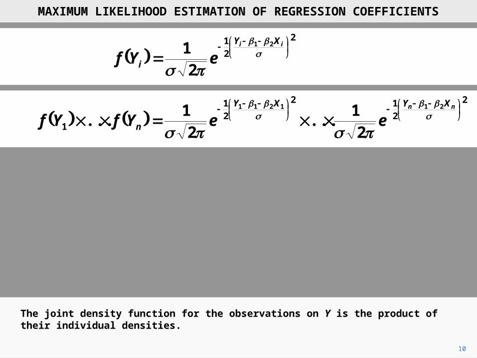
Hence the density function for the ex ante distribution of Yi is as shown.
MAXIMUM LIKELIHOOD ESTIMATION OF REGRESSION COEFFICIENTS
2
21 21
21
ii XY
i eYf
10
The joint density function for the observations on Y is the product of their individual densities.
MAXIMUM LIKELIHOOD ESTIMATION OF REGRESSION COEFFICIENTS
2
21 21
21
ii XY
i eYf
2
212
21
1
211211
21
...2
1...
nn XYXY
n eeYfYf

11
Now, taking b1, b2 and s as our choice variables, and taking the data on Y and X as given, we can re-interpret this function as the likelihood function for b1, b2, and s.
MAXIMUM LIKELIHOOD ESTIMATION OF REGRESSION COEFFICIENTS
2
21 21
21
ii XY
i eYf
2
212
21
1
211211
21
...2
1...
nn XYXY
n eeYfYf
2
212
21
121
211211
21
...2
1,...,|,,
nn XYXY
n eeYYL

12
We will choose b1, b2, and s so as to maximize the likelihood, given the data on Y and X. As usual, it is easier to do this indirectly, maximizing the log-likelihood instead.
2
21 21
21
ii XY
i eYf
2
212
21
1
211211
21
...2
1...
nn XYXY
n eeYfYf
2
212
21
121
211211
21
...2
1,...,|,,
nn XYXY
n eeYYL
2
212
21 211211
21
...2
1loglog
nn XYXY
eeL
MAXIMUM LIKELIHOOD ESTIMATION OF REGRESSION COEFFICIENTS

Zn
XYXYn
ee
eeL
nn
XYXY
XYXY
nn
nn
221
log
21
...21
21
log
21
log...2
1log
21
...2
1loglog
2
2
21
2
1211
2
212
21
2
212
21
211211
211211
13
As usual, the first step is to decompose the expression as the sum of the logarithms of the factors.
MAXIMUM LIKELIHOOD ESTIMATION OF REGRESSION COEFFICIENTS

Zn
XYXYn
ee
eeL
nn
XYXY
XYXY
nn
nn
221
log
21
...21
21
log
21
log...2
1log
21
...2
1loglog
2
2
21
2
1211
2
212
21
2
212
21
211211
211211
14
Then we split the logarithm of each factor into two components. The first component is the same in each case.
MAXIMUM LIKELIHOOD ESTIMATION OF REGRESSION COEFFICIENTS

15
Hence the log-likelihood simplifies as shown.
Zn
XYXYn
ee
eeL
nn
XYXY
XYXY
nn
nn
221
log
21
...21
21
log
21
log...2
1log
21
...2
1loglog
2
2
21
2
1211
2
212
21
2
212
21
211211
211211
221
21211 ... nn XYXYZ
MAXIMUM LIKELIHOOD ESTIMATION OF REGRESSION COEFFICIENTS
where

16
To maximize the log-likelihood, we need to minimize Z. But choosing estimators of b1 and b2 to minimize Z is exactly what we did when we derived the least squares regression coefficients.
MAXIMUM LIKELIHOOD ESTIMATION OF REGRESSION COEFFICIENTS
Zn
XYXYn
ee
eeL
nn
XYXY
XYXY
nn
nn
221
log
21
...21
21
log
21
log...2
1log
21
...2
1loglog
2
2
21
2
1211
2
212
21
2
212
21
211211
211211
221
21211 ... nn XYXYZ
where

17
Thus, for this regression model, the maximum likelihood estimators of b1 and b2 are identical to the least squares estimators.
MAXIMUM LIKELIHOOD ESTIMATION OF REGRESSION COEFFICIENTS
Zn
XYXYn
ee
eeL
nn
XYXY
XYXY
nn
nn
221
log
21
...21
21
log
21
log...2
1log
21
...2
1loglog
2
2
21
2
1211
2
212
21
2
212
21
211211
211211
221
21211 ... nn XYXYZ
where
Znn
Znn
ZnL
221
loglog
221
log1
log
221
loglog
2
2
2
18
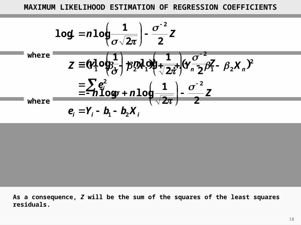
As a consequence, Z will be the sum of the squares of the least squares residuals.
MAXIMUM LIKELIHOOD ESTIMATION OF REGRESSION COEFFICIENTS
2
221
21211 ...
i
nn
e
XYXYZ
iii XbbYe 21
where
where
19
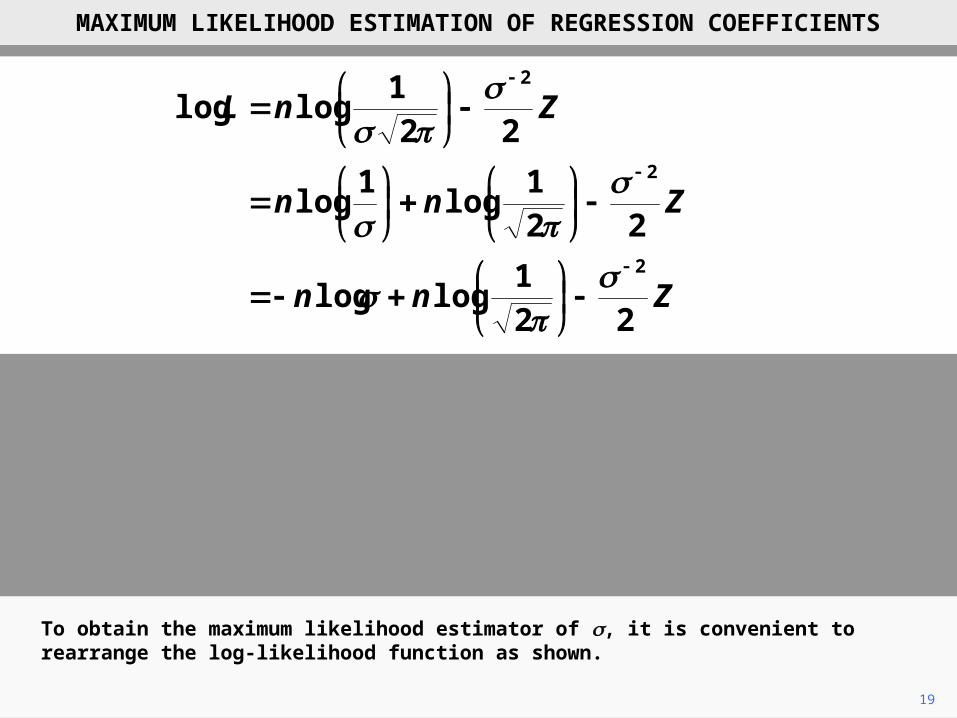
To obtain the maximum likelihood estimator of s, it is convenient to rearrange the log-likelihood function as shown.
MAXIMUM LIKELIHOOD ESTIMATION OF REGRESSION COEFFICIENTS
Znn
Znn
ZnL
221
loglog
221
log1
log
221
loglog
2
2
2

20
Differentiating it with respect to s, we obtain the expression shown.
MAXIMUM LIKELIHOOD ESTIMATION OF REGRESSION COEFFICIENTS
Znn
Znn
ZnL
221
loglog
221
log1
log
221
loglog
2
2
2
233log
nZZnL

21
The first order condition for a maximum requires this to be equal to zero. Hence the maximum likelihood estimator of the variance is the sum of the squares of the residuals divided by n.
MAXIMUM LIKELIHOOD ESTIMATION OF REGRESSION COEFFICIENTS
Znn
Znn
ZnL
221
loglog
221
log1
log
221
loglog
2
2
2
233log
nZZnL
n
e
nZ i
22̂

22
Note that this is biased for finite samples. To obtain an unbiased estimator, we should divide by n–k, where k is the number of parameters, in this case 2. However, the bias disappears as the sample size becomes large.
Znn
Znn
ZnL
221
loglog
221
log1
log
221
loglog
2
2
2
233log
nZZnL
n
e
nZ i
22̂
MAXIMUM LIKELIHOOD ESTIMATION OF REGRESSION COEFFICIENTS

Copyright Christopher Dougherty 2012.
These slideshows may be downloaded by anyone, anywhere for personal use.
Subject to respect for copyright and, where appropriate, attribution, they may be
used as a resource for teaching an econometrics course. There is no need to
refer to the author.
The content of this slideshow comes from Section 10.6 of C. Dougherty,
Introduction to Econometrics, fourth edition 2011, Oxford University Press.
Additional (free) resources for both students and instructors may be
downloaded from the OUP Online Resource Centre
http://www.oup.com/uk/orc/bin/9780199567089/.
Individuals studying econometrics on their own who feel that they might benefit
from participation in a formal course should consider the London School of
Economics summer school course
EC212 Introduction to Econometrics
http://www2.lse.ac.uk/study/summerSchools/summerSchool/Home.aspx
or the University of London International Programmes distance learning course
20 Elements of Econometrics
www.londoninternational.ac.uk/lse.
2012.12.17