Embed Size (px)
Citation preview

1
Material Requirements Planningor as we in the business like to call it - MRP
Computer Based Production Planning and Inventory Control System
Scientific Management meets the Computer

2
Where are we?
Strategic Tactical Operational
Purpose Plan acquisition of resources
Plan utilization of resources
Execution of resources
Time horizon 2+ years 6 to 24 months 1-3 months
Time period Yrs/Months Months Days/weeks
Level Top management Middle management Plant management
Questions addressed What products/LevelsPlant sizes/capacitiesPlant/warehouse locationsWhat technologies?
Inventory levelsProduction ratesWork force sizingSubcontracting
Batch sizesJob schedulingMaterial controlMachine maintenance
Analysis techniques Break-even analysis LP product mixDistribution modelsSupply Chain modelsLong range forecastingLocation analysis
ForecastingAggregate planningProduction smoothingInventory modelsFacility layoutMake or buy decisionsProject planning
Job schedulingTask sequencingAssembly line balancingShift schedulingWorker assignmentsMRP/JIT Group technologytransfer lines

3
Three Approaches to Production Controlor how much to make, when?
• Traditional– inventory control and job scheduling
• Material Requirements Planning (MRP)– along with Manufacturing Resources Planning
(MRP-II)– capacity requirements planning (CRP),– and Enterprise Resource Planning (ERP)
• Just-in-Time (JIT) Manufacturing
4
Basic Definitions
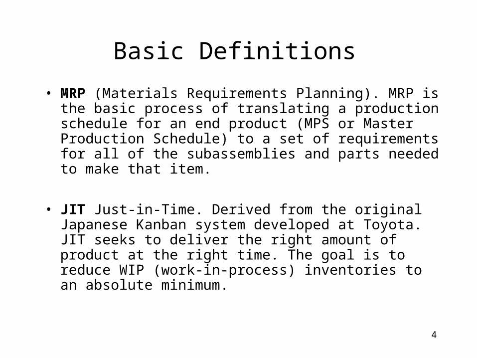
• MRP (Materials Requirements Planning). MRP is the basic process of translating a production schedule for an end product (MPS or Master Production Schedule) to a set of requirements for all of the subassemblies and parts needed to make that item.
• JIT Just-in-Time. Derived from the original Japanese Kanban system developed at Toyota. JIT seeks to deliver the right amount of product at the right time. The goal is to reduce WIP (work-in-process) inventories to an absolute minimum.
5
Why Push and Pull?
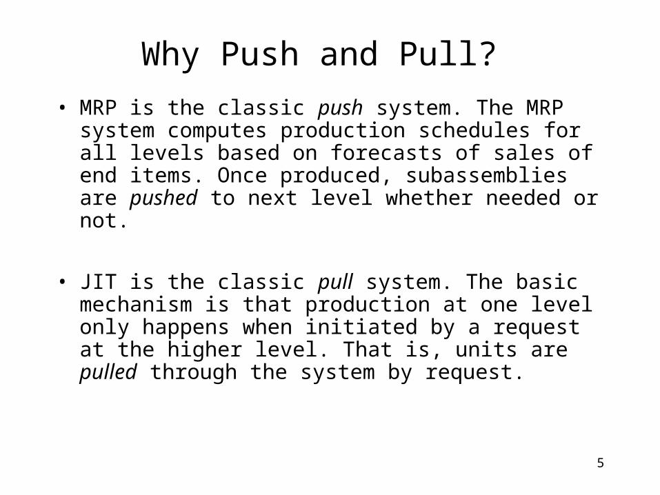
• MRP is the classic push system. The MRP system computes production schedules for all levels based on forecasts of sales of end items. Once produced, subassemblies are pushed to next level whether needed or not.
• JIT is the classic pull system. The basic mechanism is that production at one level only happens when initiated by a request at the higher level. That is, units are pulled through the system by request.

6
Push versus Pull
•Push – MRP•Forecast driven•Production Plan by period•Parts – explosion•Uses lot-sizing techniques
•Pull – JIT•Production driven by demands (in the form of Kanban) from the next higher level•Minimizes work-in-process•Requires reduced setup times

7
Advantages
MRPreacts to changes in demandsallows for lot sizing to reduce setup costsplans for several time periods into the future
JITreduces work-in-processquickly identify quality problems before large inventories of defect partssmooth flow of material through the supply chain

8
What problem does MRP try to solve?
• Independent demand – originates outside the factory system– Is subject to uncertainty
– Traditional (stochastic) inventory models work well
• Dependent Demand – demand for components that make up independent demand products– No uncertainty – demand is known (at least in
principle) once the final assembly schedule is given
– Traditional (stochastic) inventory models do not work well

9
MRP versus JIT – an Example
• Assembly of a garden spade requires two screws.• Spades are assembled in batches of 400 on the
first two days of every month• The weekly demand pattern for screws therefore
is:800,0,0,0, 800,0,0,0, 800,0,0,0, 800,0,0,0, etc.

10
The MRP Approach
• Using a weekly demand rate of 200, say, holding and setup costs are such that the EOQ solution is Q* = 1,400.– solution makes no sense since 600 would be stored for
3 weeks and then another order placed for 1,400– Treating weekly demand as random makes no sense as
well since it is deterministic• Order 10,400 at the beginning of the year and
incur only one fixed order and delivery cost per year
• Ideally use dynamic lot sizing based on costs– i.e. order some multiple of 800

11
The JIT Approach
• Schedule delivery of 800 screws at the beginning of each month– Incur fixed ordering cost 12 times a year
– No inventory to store
– If usage varies, can modify delivery sizes
– If a defective shipment only screwed for 800 screws
• To be economical, fixed order and delivery costs must be small

12
MRP Objectives
• Insure availability of materials, component, and products
• Maintain lowest possible inventory level
• Plan manufacturing activities, delivery schedules, and purchasing requests
An MRP fact:“MRP deals with two basic dimensionsin production: Quantities and Timing”

13
Forecast of future demand
Production Planning
Master Production ScheduleSchedule of production quantities byProduct (end item) and time period
Materials requirements planning systemExplode master schedule to obtain requirementsfor assemblies, components, and raw material
Time-phasedWork orders
Lot sizingand capacityplanning
Time-phasedPurchase orders
The MRP System
Customerorders
planned-orderreleases

14
Input 1 - Master Production Schedule
• This is the forecast for the sales of the end item over the planning horizon. The data sources for determining the MPS include: – Firm customer orders– Forecasts of future demand by item– Safety stock requirements– Seasonal variations– Internal orders from other parts of the
organization.

15
Input 2 - Bill of Materials
Bill of materials• parent-child (hierarchical) relationships• quantity per application (QPA)• production or procurement lead-times

16
Input 3 – Inventory Position
• For all items at all levels for each time period– On-hand inventory quantities– On-order quantities (due-in’s)
Let’s see. We have 3 of these with 5 more arriving on the 23rd.

17
Input - Output
1. Master Production Schedule2. Bill of Materials and level codes3. Inventory status of all items – on-hand and on-order
MRP SYSTEM
Compute for all components:• Gross requirements• Planned order and work releases• Time phasing of net requirements

18
A Three-legged Stool
StoolFinal assembly area
1 seat assemblyDepartment X
1 seatDept X
leg assemblyDepartment Y
3 legsDept Y
6 screwsVendor A
End item
Parent level
Child level 3 supportsDept Y
1 cushionVendor B
6 screwsVendor A
Raw material – lumber - Paul Bunyon Lumber Co.

19
VendorLead-times
One week
One week
Two weeks
A Three-legged Stool
StoolFinal assembly area
1 seat assemblyDepartment X
1 seatDept X
leg assemblyDepartment Y
3 legsDept Y
6 screwsVendor A
ProductionLead-timesOne week
One week
Two weeks 3 supportsDept Y
1 cushionVendor B
6 screwsVendor A
Raw material – lumber - Paul Bunyon Lumber Co.

20
A Three-legged Stool
StoolFinal assembly area
seat assemblyDepartment X
1 seatDept X
leg assemblyDepartment Y
3 legsDept Y
6 screwsVendor A
Independent Demand
3 supportsDept Y
1 cushionVendor B
6 screwsVendor A
Raw material – lumber - Paul Bunyon Lumber Co.
Dependent Demand

21
Lumpy Demands due to lot sizing
Time period 1 2 3 4 5 6Assembly Xdemand 10 10 10 10 10 10Production 30 30Assembly Y 5 5 5 5 5 5Production 10 10 10Assembly Z 7 7 7 7 7 7Production 7 7 7 7 7 7Subassembly ARequirements 57 7 27 37 27 7
Assemblies X and Z require one unit of assembly A while Assembly Y requires two.
dependentdemand
time buckets
SubAsbAper 1 = 30 + 2 (10) + 7 = 57

22
Terminology
• bill of materials – all parent-child relationships
• level coding – the order in which the requirements must be computed (indenture level)
• lead-time offset – due date minus the planned order release date

23
Product Structure
A
B d(2)
2
D B g(3)
C
d f(3)
B
g C(2)
1
A(2) C
D
B(2) C
Two end products (1 and 2)Four assemblies (A, B, C, and D)Three parts (d, f, and g)
( ) – indicates number of components used on next higher assembly

24
Bill of Materials Matrix - B
End partsProduct subassemblies (components)1 2 A D B C g d f
1 2 12 1 1 3
A 1 2D 2 1B 2 1C 1 3
dfg
Why this is an upper triangular matrix isn’t it!

25
MRP Level Assignments
A
B d(2)
2
D B
C
d f(3)
B
g C(2)
1
A(2) C
D
B(2) C
Level 01, 2
Level 1A, D
Level 2B
Level 3C, g
Level 4d, f
g(3)
use topological sorting

26
Topological Sorting
13
9
74
2
58
1
3
6
7
4
2
5
8
96
rearrange so allarrows go down
note: no loops are present

27
Computing Direct Dependent Demands
Let Dn = vector of dependent demand directly resultingfrom demand at level n (output vector)
dn = vector of demand at level n (input vector)
Then Dn = dn x B where B is the Bill of Materials Matrix
and D0 = d0 B; D1 = d1B = D0 B = (d0 x B x B); D2 = d2 B = (d0 x B x B x B); etc.
Then total demand = D0 + D1 + … + Dm
= d0 x (B + B2 + B3 + … + Bm )

28
0 0 2 0 0 1 0 0 0
0 0 0 1 1 0 3 0 0
0 0 0 0 1 0 0 2 0
0 0 0 0 2 1 0 0 0
0 0 0 0 0 2 1 0 0
0 0 0 0 0 0 0 1 3
0 0 0 0 0 0 0 0 0
0 0 0 0 0 0 0 0 0
0 0 0 0 0 0 0 0 0
D0 = d0 B
= (100, 200, 0, 0, 0, 20, 0, 0, 0) x
= (0, 0, 200, 200, 200, 100, 600, 20, 60) = d1
Requirement: A D B C g d f200 200 200 100 600 20 60
1 2 A D B C g d f
1 2 A D B C g d f
Assume independent demand for item 1 = 100 units & item 2 = 200 unitsand there is a spare part demand for 20 C’s.

29
0 0 2 0 0 1 0 0 0
0 0 0 1 1 0 3 0 0
0 0 0 0 1 0 0 2 0
0 0 0 0 2 1 0 0 0
0 0 0 0 0 2 1 0 0
0 0 0 0 0 0 0 1 3
0 0 0 0 0 0 0 0 0
0 0 0 0 0 0 0 0 0
0 0 0 0 0 0 0 0 0
D1 = d1 B
= (0, 0, 200, 200, 200, 100, 600, 20, 60) x
= (0, 0, 0, 0, 500, 500, 200, 100, 300) = d2
Requirement: A D B C g d f0 0 500 500 200 500 300
1 2 A D B C g d f
1 2 A D B C g d f
Level 2 requirement

30
Computing Total Requirements
21 1 2 2 , 1 1,
1
...n
ij ik kj i j i j i i i jk
b b b b b b b b b
by matrix multiplication of B x B:
If B is an n x n triangular matrix, then Bk = 0 for any k n
If i j then b2i,j = 0

31
0 0 2 0 0 1 0 0 0
0 0 0 1 1 0 3 0 0
0 0 0 0 1 0 0 2 0
0 0 0 0 2 1 0 0 0
0 0 0 0 0 2 1 0 0
0 0 0 0 0 0 0 1 3
0 0 0 0 0 0 0 0 0
0 0 0 0 0 0 0 0 0
0 0 0 0 0 0 0 0 0
0 0 2 0 0 1 0 0 0
0 0 0 1 1 0 3 0 0
0 0 0 0 1 0 0 2 0
0 0 0 0 2 1 0 0 0
0 0 0 0 0 2 1 0 0
0 0 0 0 0 0 0 1 3
0 0 0 0 0 0 0 0 0
0 0 0 0 0 0 0 0 0
0 0 0 0 0 0 0 0 0
B2 =
0 0 0 0 2 0 0 5 3
0 0 0 0 2 3 1 0 0
0 0 0 0 0 2 1 0 0
0 0 0 0 0 4 2 1 3
0 0 0 0 0 0 0 2 6
0 0 0 0 0 0 0 0 0
0 0 0 0 0 0 0 0 0
0 0 0 0 0 0 0 0 0
0 0 0 0 0 0 0 0 0
= Therefore b21,8 = 5 is the
level 1 requirement for component d in product 1.

32
MRP Level Assignments
A
B d(2)
2
D B
C
d f(3)
B
g C(2)
1
A(2) C
D
B(2) C
Level 01, 2
Level 1A, D
Level 2B
Level 3C, g
Level 4d, f
g(3)

33
0 0 2 0 0 1 0 0 0
0 0 0 1 1 0 3 0 0
0 0 0 0 1 0 0 2 0
0 0 0 0 2 1 0 0 0
0 0 0 0 0 2 1 0 0
0 0 0 0 0 0 0 1 3
0 0 0 0 0 0 0 0 0
0 0 0 0 0 0 0 0 0
0 0 0 0 0 0 0 0 0
0 0 0 0 0 4 2 0 0
0 0 0 0 0 4 2 2 9
0 0 0 0 0 0 0 2 6
0 0 0 0 0 0 0 4 12
0 0 0 0 0 0 0 0 0
0 0 0 0 0 0 0 0 0
0 0 0 0 0 0 0 0 0
0 0 0 0 0 0 0 0 0
0 0 0 0 0 0 0 0 0
B3 =
0 0 0 0 2 0 0 5 3
0 0 0 0 2 3 1 0 0
0 0 0 0 0 2 1 0 0
0 0 0 0 0 4 2 1 3
0 0 0 0 0 0 0 2 6
0 0 0 0 0 0 0 0 0
0 0 0 0 0 0 0 0 0
0 0 0 0 0 0 0 0 0
0 0 0 0 0 0 0 0 0
= Therefore b32,9 = 9 is the
level 2 requirement for component f in product 2.

34
Let ri,j = total number of units of item j required toproduce one unit of item i where ri,i = 1 by definition. therefore:
R = I + B + B2 + B3 + … + Bn + 0 + …
recall:
Therefore R = (I – B)-1
1
0
1(1 )
1n
n
x xx
Total Requirements matrix (R)

35
0 0 2 0 0 1 0 0 0
0 0 0 1 1 0 3 0 0
0 0 0 0 1 0 0 2 0
0 0 0 0 2 1 0 0 0
0 0 0 0 0 2 1 0 0
0 0 0 0 0 0 0 1 3
0 0 0 0 0 0 0 0 0
0 0 0 0 0 0 0 0 0
0 0 0 0 0 0 0 0 0
B =
1 0 2 0 2 5 2 9 15
0 1 0 1 3 7 6 7 21
0 0 1 0 1 2 1 4 6
0 0 0 1 2 5 2 5 15
0 0 0 0 1 2 1 2 6
0 0 0 0 0 1 0 1 3
0 0 0 0 0 0 1 0 0
0 0 0 0 0 0 0 1 0
0 0 0 0 0 0 0 0 1
R = (I – B)-1 =

36
let d = vector of independent demands which includes demands forend products, spare assemblies, and spare components
Q = total production requirements vector
then Q = d R = d (I – B)-1
1 0 2 0 2 5 2 9 15
0 1 0 1 3 7 6 7 21
0 0 1 0 1 2 1 4 6
0 0 0 1 2 5 2 5 15
0 0 0 0 1 2 1 2 6
0 0 0 0 0 1 0 1 3
0 0 0 0 0 0 1 0 0
0 0 0 0 0 0 0 1 0
0 0 0 0 0 0 0 0 1
Q = d R = (20, 30, 0, 10, 0, 5, 0, 0, 0) x
= (20, 30, 40, 40, 150, 365, 240, 445, 1095)
item 1 2 A D B C g d fdemand 20 30 0 10 0 5 0 0 0

37
d R = (100, 200, 0, 0, 0, 20, 0, 0, 0) x
1 0 2 0 2 5 2 9 15
0 1 0 1 3 7 6 7 21
0 0 1 0 1 2 1 4 6
0 0 0 1 2 5 2 5 15
0 0 0 0 1 2 1 2 6
0 0 0 0 0 1 0 1 3
0 0 0 0 0 0 1 0 0
0 0 0 0 0 0 0 1 0
0 0 0 0 0 0 0 0 1
= (100, 200, 200, 200, 800, 1920, 1400, 2320, 5760)
Requirement:A D B C g d f200 200 800 1920 1400 2320 5760
from earlier example:

38
MRP Procedure• Netting: Determine net requirements
– gross requirements –[on-hand inventory + scheduled receipts]
• Establish lot sizes– divide net requirements into production lots or order quantities
• Time Phasing: Determine planned order release dates– Offset due dates with lead-times
• BOM Explosion: Expand to next level– Generate gross requirements of all components on next level
• Iterate: Repeat until all levels have been processed.

39
Master Production Scheduling
Qj,t = scheduled receipts (order or lot size quantity) of item j during period t
Rj,t = gross requirement of item j during period tIj,t = expected on-hand inventory of item j at the beginning of period tNj,t = net requirements for item j in period t
Note: Rj,t = max{ forecast for period t, customer orders period t}
Nj,t = max{0, Rj,t – Qj,t – Ij,t}

40
Master Production Scheduling (cont.)
Ij,t = expected on-hand inventory of item j at the beginning of period t
Qj,t = scheduled receipts (order or lot size quantity) of item j during period t
Rj,t = gross requirement of item j during period t
, 1 , 1 , 1max 0,jt j t j t j tI I Q R
41
MRP - Example
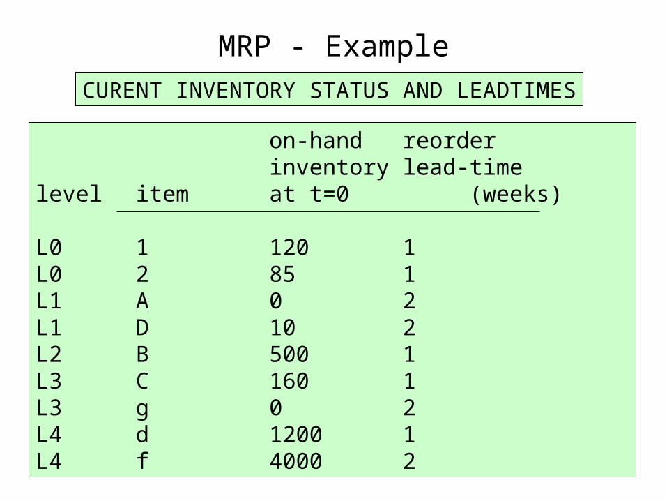
CURENT INVENTORY STATUS AND LEADTIMES
on-hand reorderinventory lead-time
level item at t=0 (weeks)
L0 1 120 1L0 2 85 1L1 A 0 2L1 D 10 2L2 B 500 1L3 C 160 1L3 g 0 2L4 d 1200 1L4 f 4000 2

42
Example - demands Week 1 2 3 4 5 6 7 8
9Item I1 50 20 30 40 40 30 25 15
30I2 20 30 25 35 10 35 20 25
30A 15D 10 10B 20
100C 5gdf
Master Production Schedule

43
Example – level 0Week 1 2 3 4 5 6 7 8 9Item 1R1 50 20 30 40 40 30 25 15 30Q1 120I1 120 70 50 20 100 60 30 5 0N1 10 30OR 120 120
Week 1 2 3 4 5 6 7 8 9Item 2R2 20 30 25 35 10 35 20 25 30Q2 100I2 85 65 35 10 75 65 30 10 0N2 15 30OR 100 100
OR – order releases(based on lot-sizes of 120 and 100)

44
0 0 2 0 0 1 0 0 0
0 0 0 1 1 0 3 0 0
0 0 0 0 1 0 0 2 0
0 0 0 0 2 1 0 0 0
0 0 0 0 0 2 1 0 0
0 0 0 0 0 0 0 1 3
0 0 0 0 0 0 0 0 0
0 0 0 0 0 0 0 0 0
0 0 0 0 0 0 0 0 0
D0 = d0 B
= (120, 100, 0, 0, 0, 0, 0, 0, 0) x
= (0, 0, 240, 100, 100, 120, 300, 0, 0)
Gross
Requirement: A D B C g240 100 100 120 300
Gross requirements –lower level period 7

45
Example – level 1
Week 1 2 3 4 5 6 7 8 9Item AR 0 0 240 0 0 0 240 15 0Q 240I 0 0 0 0 0 0 0 0 0N 240 15OR 240 240 15
OR – order releases(based on lot-sizing)
Week 1 2 3 4 5 6 7 8 9Item DR 0 10 100 10 0 0 100 0 0Q 100 10I 10 10 0 0 0 0 0 0 0N 100OR 100 10 100
lead-time2 weeks
note: lot for lot re-order policy

46
0 0 2 0 0 1 0 0 0
0 0 0 1 1 0 3 0 0
0 0 0 0 1 0 0 2 0
0 0 0 0 2 1 0 0 0
0 0 0 0 0 2 1 0 0
0 0 0 0 0 0 0 1 3
0 0 0 0 0 0 0 0 0
0 0 0 0 0 0 0 0 0
0 0 0 0 0 0 0 0 0
D1 = d1 B
= (0, 0, 240, 100, 0, 0, 0, 0, 0) x
= (0, 0, 0, 0, 440, 100, 0, 480, 0)
Gross
Requirement: B C d440 100 480
Gross requirements –lower levels period 5

47
MRP Level Assignments
A
B d(2)
2
D B
C
d f(3)
B
g C(2)
1
A(2) C
D
B(2) C
Level 01, 2
Level 1A, D
Level 2B
Level 3C, g
Level 4d, f
g(3)
use topological sorting
48
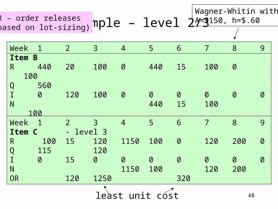
Example – level 2/3
Week 1 2 3 4 5 6 7 8 9Item BR 440 20 100 0 440 15 100 0 100Q 560I 0 120 100 0 0 0 0 0 0N 440 15 100 100OR 555 100
OR – order releases(based on lot-sizing)
Wagner-Whitin withA=$150, h=$.60
Week 1 2 3 4 5 6 7 8 9Item C - level 3R 100 15 120 1150 100 0 120 200 0Q 115 120I 0 15 0 0 0 0 0 0 0N 1150 100 120 200OR 120 1250 320
least unit cost

49
Example – level 3/4
Week 1 2 3 4 5 6 7 8 9Item g - level R 0 0 300 575 0 0 300 100 0Q 300I 0 0 0 0 0 0 0 0 0N 575 300 100OR 300 575 300 100
Week 1 2 3 4 5 6 7 8 9Item d - level 4R 480 120 1250 0 480 350 0 0 0QI 1200 720 600 600 120 0 0 0 0N 230OR
OR – order releases(based on lot-4-lot)

50
Example – level 4
Week 1 2 3 4 5 6 7 8 9Item f - level 4R 0 360 3750 0 0 960 0 0 0Q 110I 4000 4000 3640 0 0 0 0 0 0N 960OR 110 960
This is a great level.

51
Lot sizing and MRP
least unit cost heuristic: Inv Unit net lot weeks carry-cost $ per Setup Total
period rqmt size in inv per lot Unit Cost (unit)
wk 4 1150 0 0 0 0 .87 .87wk 5 100 1250 1 60 .05 .80 .85wk 6 0 2wk 7 120 1370 3 276 .20 .73 .93wk 8 200 1570 4 756 .48 .64 1.12
Iteration 2wk 7 120 120 0 0 0 8.33 8.33wk 8 200 320 1 120 .38 3.13 2.51
setup cost = $1000holding cost = .60 /unit-periodunit cost = $1
item C periods 4 - 8

52
Lot Sizing with Capacity Constraints
Known requirements in each period versus capacitiesri = requirement in period ici = production capacity in period iyi = production level in period i
1 2
1 2
1 2
, ,...,
, ,...,
, ,..., , 1
n
n
n i i
r r r
c c c
Find y y y where y c for i n
1 1
1,...,j j
i ii i
c r for j n

53
Example 7.7
r = (20, 40, 100, 35, 80, 75, 25)c = (60, 60, 60, 60, 60, 60, 60)
periodadditive
rqmtAdditive capacity
1 20 602 60 1203 160 1804 195 2405 275 3006 350 3607 375 420
Check for feasibility:

54
The simple 2-step algorithm1. Find next period in which demand > capacity
2. Back-shift demands to period(s) having excess capacity
0. r = (20, 40, 100, 35, 80, 75, 25)c = (60, 60, 60, 60, 60, 60, 60)
1. 40 60 60r = (20, 40, 100, 35, 80, 75, 25)c = (60, 60, 60, 60, 60, 60, 60)
2. 40 60 60 55 60r = (20, 40, 100, 35, 80, 75, 25)c = (60, 60, 60, 60, 60, 60, 60)
3. 50 60 40 60 60 55 60 60 25r = (20, 40, 100, 35, 80, 75, 25)c = (60, 60, 60, 60, 60, 60, 60)
Final answer:y = (50, 60, 60, 60, 60, 60, 25)
Feasible but not necessarily optimal!

55
The Improvement 2-Step• Start at end and work backwards
• Determine if it is cheaper to shift entire production lot to prior periods having excess capacity
Assume k = $450 and h = $2:
0. r = (100, 79, 230, 105, 3, 10, 99, 126, 40) c = (120, 200, 200, 400, 300, 50, 120, 50, 30)
1. r’ = (100, 109, 200, 105, 28, 50, 120, 50, 30) c = (120, 200, 200, 400, 300, 50, 120, 50, 30)Cost = 9 x 450 + 432 = $4,482
2. r’= (100, 109, 200, 105, 28, 50, 120, 50, 30) c = (120, 200, 200, 400, 300, 50, 120, 50, 30) y = (100, 109, 200, 105, 58, 50, 120, 50, 0)Cost = 8 x 450 + (432 + 2 x 30 x 4) = $4,272
Look for improvement
Find feasible solution

56
More Improvement• Start at end and work backwards
• Determine if it is cheaper to shift entire production lot to prior periods having excess capacity
Assume k = $450 and h = $2:
1. r’ = (100, 109, 200, 105, 28, 50, 120, 50, 30) c = (120, 200, 200, 400, 300, 50, 120, 50, 30)Cost = 9 x 450 + 432 = $4,482
2. r’= (100, 109, 200, 105, 28, 50, 120, 50, 30) c = (120, 200, 200, 400, 300, 50, 120, 50, 30) y = (100, 109, 200, 105, 58, 50, 120, 50, 0)Cost = 8 x 450 + (432 + 2 x 30 x 4) = $4,272
2. r’= (100, 109, 200, 105, 28, 50, 120, 50, 30) c = (120, 200, 200, 400, 300, 50, 120, 50, 30) y = (100, 109, 200, 105, 108, 50, 120, 0, 0)Cost = 7 x 450 + (432 + 240 + 300) = $4,122
Let’s do another one…

57
Do it again?Assume k = $450 and h = $2:
2. r’= (100, 109, 200, 105, 28, 50, 120, 50, 30) c = (120, 200, 200, 400, 300, 50, 120, 50, 30) y = (100, 109, 200, 105, 108, 50, 120, 0, 0)Cost = 7 x 450 + (432 + 240 + 300) = $4,122
2. r’= (100, 109, 200, 105, 28, 50, 120, 50, 30) c = (120, 200, 200, 400, 300, 50, 120, 50, 30) y = (100, 109, 200, 105, 228, 50, 0, 0, 0)
Savings = $450Cost = $2 x 120 x 2 = $480
No! Don’t do it. It will cost
more.
Look at shifting 50 units in period 6 to period 5 and the resulting 158 units in period 5 to period 4Final answer: y = (100, 109, 200, 263, 0, 0, 0, 0, 0) with cost = $3,638

58
There are still problems…
The problem is that even if lot sizes at some level do not exceed production capacities, there is no guarantee that
when these lot sizes are translated into gross requirements at a lower level, that they will not exceed capacities.

59
Optimal Multi-level Lot Sizing
1 1
N T
i it i iti t
Min A z h I
1,( 1) 1 1
,( 1) , ( ) ( ),
1
0 1 , 2
1 , 2
, 0, 0 1
t t t t
i t it it i s i s i t
it it
it it it
I Q I R for t T
I Q I m Q for t T i N
Q z M for t T i N
Q I z or
subject to:
let AI = setup cost for item ihi = holding cost for item iIit = inventory level ending period tQit = order quantity of item i, period tzit = 1 if item i is ordered period t; otherwise 0mi,s(i) = number units of i required to produce s(i)Rt = end item requirement in period t

60
Weaknesses and Problems
• assumes infinite production capacity– MRP identifies what is to be done to meet the master
schedule– capacity planning usually occurs after the fact– capacity lot-sizing at one level will not solve overall
capacity problem• deterministic system
– lead-times & demands– lead-times do not consider plant loading– lead-times are inflated to compensate creating more
problems– lead-times may be dependent on lot sizes
MRP is based upon a flawed model!

61
System NervousnessCaused by Rolling Horizon
Only 1st period decision of a N-period problem is implemented.Using the Wagner-Whitin algorithm:
t 1 2 3 4 5Dt 190 210 190 210 190Qt 190 400 0 400 0
A = $400 / orderh = $1 per item
t 1 2 3 4 5 6Dt 190 210 190 210 190 210Qt 400 0 400 0 400 0
Q1 = 190 if odd number of periodsQ1 = 400 if even number of periods

62
More Problems
• Random numbers of defective items• Data Integrity
– machine unavailability
– engineering changes
– discrepancies in inventory records
– changes in demands (forecasts), costs, or lead-times
• Lead-times dependent upon lot sizes• Reject or rework rates must be addressed

63
After MRP?• MRP II – Manufacturing Resource Planning
– includes MRP-I– adds financial, accounting, and marketing functions– MPS becomes a decision variable– capacity resource planning (CRP) an integral feature
• ERP – Enterprise Resource Planning– includes MRP-II– entire firm operates on the same data– client-server with a single relational database– multi-location (international) support– includes customer orders, distribution, delivery
schedules, etc.

64
More on ERP
• Enterprise systems are commercial software packages that enable the integration of transactions-oriented data and business processes throughout an organization (and perhaps eventually throughout the entire inter-organizational supply chain).
• Enterprise systems include ERP software and related packages as advanced planning and scheduling (APS), sales force automation, customer relationship management, product configuration, etc.)

65
More of More on ERP
• Most companies have failed to implement ERP packages successfully or to realize the hoped-for financial returns on their ERP investment.
• Standish Group Study of ERP Implementations:– 35% are Cancelled– 55% overrun their budgets– Less than 10% are on time and under budget
• Implementation Averages– Cost: 178% over budget– Schedule: 230% longer– Functionality: –59% or: the system will only perform
41% of the functions it was intended to perform.

66
Why Implementations Fail
• People Don’t want the systems to succeed• People are comfortable and don’t see the need
for the new system.• People have unrealistic expectations of the new
system.• People don’t understand the basic concepts of
the system.• The basic data is inaccurate.• The system has technical difficulties.

67
What about APS?
• APS is Advance Planning and Scheduling:
The technique that deals with analysis and planning of logistics and manufacturing over the short, intermediate and long-term periods. APS describes any computer program that uses advanced mathematical algorithms or logic to perform optimization or simulation on finite capacity scheduling, sourcing, capital planning, resource planning, forecasting, demand management and others.

68
The Five Main Components Of an APS System
• demand planning
• production planning
• production scheduling
• distribution planning
• transportation planning
Gosh there are five of them.

69
MRP and APS
• APS considers all constraints and capacities simultaneously using mathematical models (linear programming or some derivative) and yields a production plan (either short term or longer term).
• MRP can take this plan and execute the acquisition of materials.
• MRP is more transaction focused and an older product than APS
• APS is more modeling oriented.

70
Homework
From your textbook: chapter 7: 4,5,6,23,24,25,27,28 + handout
Hey! This MRP stuff is okay. Can we have some homework problems to try it out? Please.