1 Log-Graph software

Version 1.0.1

The software enables the operation of the loggers 100/110 on a PC running Windows operating system via a vacant USB port. It undertakes the setting of the logger and the readout/display and archiving of recorded data. The parameters include all the functions available in the logger.

The content gives an overview of all functions of the Log-Graph software. You will find an index at the end of the manual.

1 Log-Graph 1.1 Contents

2 Introduction

2.1 Functional scope of the logger 2.2 Functional scope of the software

2.2.1 Logger settings 2.2.2 Logger status 2.2.3 Records 2.2.4 Actions

2.3 System requirements 2.4 Content of the software package 2.5 Installing the Log-Graph software

2.5.1 Installing the CD 2.5.2 Installing the downloads from the Internet 2.5.3 Installing the USB driver for logger operation on the USB port

2.5.3.1 Installation 2.5.3.2 Renaming the port

2.6 Communication between the PC and the logger 2.7 First connection of a device

3 Working with the Log-Graph software

3.1 Using the program menu 3.2 Using the device bar 3.3 Online view 3.4 Graph area 3.5 Status line

4 Basic settings for the software operation

5. Presentation of graphs and tables

5.1 Graph (without table) 5.2 Graph and table side by side 5.3 Table (without graph) 5.4 Functions for graph processing

5.4.1 Functions from the menu or the toolbar 5.4.2 Functions by using the mouse 5.4.3 Printing the graphs and the records

5.5 Window management

6. Log-Graph editor

6.1 Special editor functions in the active device window

Annex

Version overview

2 Introduction

This manual describes the installation of the Log-Graph software and its use in conjunction with the loggers 100/110. The software enables the operation of the loggers 100/110 on a PC running Windows operating system via a vacant USB port. It undertakes the setting of the logger and the readout of recorded data and supports all the fonctions available in the logger. The loggers 100 and 110 are distinguishable from each other by the fact that the first one incorporates a pure temperature sensor while the second one has a combined temperature and humidity sensor. The logger 100 only provides raw temperature data, the logger 110 provides both temperature and humidity data from which the dew point is calculated. An additional external temperature sensor may be connected to both loggers via the vacant USB port. The logger can only be operated using the buttons Start/Stop und Mode. The setting of the logger and the readout of the recorded data must be performed via the Log-Graph software on the PC.

The connection of the logger to the PC is made using an appropriate USB cable plugged into an available USB Port. When connecting the logger, the USB port is configured as virtual COM port from 1-256 via the drivers installed. The logger is handled by the Log-Graph software as a device on a serial port. This requires the installation of Windows drivers which are located on the installation CD of Log-Graph (installation see 2.7.3 "Installing the drivers"). The paragraphs 2.1 to 2.6 describe the properties of the logger and the software, the paragraph 2.7 describes how to install the drivers and the software.

Properties of the logger and the software

2.1 Functional scope of the logger

The loggers 100/110 have the following properties:

� Temperature (internal) with a resolution of up to 0.1 ° C / ° F � Humidity (only 110) with a resolution of 0.1% RH � Connection for external temperature sensor (via the USB connector) � internal logger clock with date/ time �Up to 60,000 records with intervals of 1 sec to 24 hours � Display of Min / Max / Avg values via the Mode button or automatically � Limit value monitoring and display via the LED and the beeper � Start and stop via a) Start/Stop button b) Time indication c) Duration or record number � Power saving functions

2.2 Functional scope of the software

The software is used to set the logger operating parameters, to read out and archive the recorded data and display the operating status. The following functions are available:

2.2.1 Logger settings:

� Read and set the real time clock in the logger � Display of the battery‘s charge state � Read and set the recording interval � Configure the memory (record number/circular memory) � Start and stop the recording � Start indications: time/button/Reed relay (option)/immediate startup and protection against

multiple startup � Stop indications: time/duration/record number/button/Reed relay (option)/endless (circular

memory) � Set the limit values and their handling (LED/beeper), alarm delay, alarm accumulation � Activate the external sensor � Units °C or °F � Power saving settings for the LCD display, the LEDs and the beeper � Update intervals for the LCD display, the LED flashes and the beeper � Button lock for the Mode button � Entry of up to eight user-defined names

2.2.2 Logger status:

� Overview of the hardware and the logger ID � Overview of the operating status of the logger � Log entries of the limit value exceedings and the errors occurred � Overview of all the parameters available in the logger

2.2.3 Records:

� Instantaneous value display during the recording process � Readout of the recorded data � Presentation in tabular and graphic form � Adding of notes on existing records � Printing of records (table or graph)/notes as report

2.2.4 Operations:

� Configuration of the USB port (automatic search) � Start and stop of the logger via PC � Reset to basic settings � Saving and loading of the logger settings 2.3 System requirements

The software is designed to run on Windows-based PCs (from Win 98 onwards, Win ME, 2000, XP, Vista, Win 7). The installation requires the following conditions: • Standard PC from 386 onwards with a keyboard and mouse (or equivalent pointing device) • CD-ROM drive (for installation), or Internet access (for installation) • an available USB port • Graphic resolution 800 x 600 or higher • approx. 10 MB of free hard disk space for installation • a logger LOG 100 or LOG 110

A 32-bit Windows operating system (at least from Win98 onwards) or a more modern Windows ® operating system (32/64-bit) must be installed on the PC. Based on our experience, a safe operation of the operating system installed is a prerequisite for proper functioning of the Log-Graph software.

2.4 Content of the software package

The software package includes the following components

� the installation routine German / English / French � the program German (later also in English / French) � help files German (and later English / French) � the manual in PDF format German (later also in English / French) � drivers for use of the logger on the USB port

With a download of the software, the volume is identical. All the files mentioned above are also included in Setup.exe. The following manuals may be useful for an easy and fast installation as well as commissioning of the Log-Graph software on the respective PC operating system:

- The Microsoft Windows® user guide corresponding to the operating system - The instruction manual of the logger 100/110 corresponding to the device used

Communication between the PC and the logger

To communicate, the logger and the PC use a USB port which is configured as serial COM port from 1-256 via the drivers (similar to a USB serial adapter). The properties of this port match those of a serial port at 115200 baud, 8 data bits, 1 stop bit and no parity. Some functions can be tested using the additional program included in Windows accessories "Hyper-terminal". These include the following functions: "* IDN? "- gives a string with the IDs of the logger, "* TST? - gives "0" if the logger is available, "-1" in case of communication problems or "* RST" - performs a soft reset of the logger.

In addition, many other commands are used in conjunction with certain parameters to exchange data with the logger. Their explanation is not part of this documentation, and would fill many more pages - this remark only completes the information previously provided. Currently, there are no plans to disclose the commands and the protocols hidden behind them. The logger provides access to many internal parameters via a direct addressing of the appropriate memory cell and reading of the data stored therein. Conversely, the parameters may similarly be addressed and overwritten by the PC. Besides the data transmitted, a checksum confirming the safety of the data transmitted is also transmitted with each communication. The protocol itself is not currently disclosed. When downloading (reading out) the recorded data, a protocol encrypting the transmission of a record in blocks of 5 bytes each (mode Penta) is used. During the readout, all existing records are transmitted in one go as dump. The dump starts with a header that contains the record number. Next come all the records. A checksum also follows at the end of the entire transmission. This procedure is not currently disclosed. Once launched, a dump can still be interrupted by the PC, however the data are preserved in the logger. In general, during the readout of records, no data is deleted from the logger, so that the readout process can be repeated as often as you wish, as long as the records have not been replaced by a newly launched record.

2.6 First connection of a device

• To commission the logger, proceed as described in the instruction manual (insert the battery or remove the protective film). The logger is ready to operate and can be connected to the PC.

• Connect the logger to the PC via the USB connection cable.

• When you connect the logger for the first time, there no drivers available. When the computer is on or after connecting the logger, the operating system detects a "new unknown hardware" and wants to install the necessary drivers. They are on the CD or, if the software has already been installed, in the folder "Drivers" of the program directory where the software was installed.

• For this purpose, proceed as described in "Installing the USB driver".

Installing the drivers and the software

2.7 Installing the Log-Graph software

The Log-Graph software is delivered on CD or its newest version can be downloaded from the Internet. To operate the logger on the PC, a driver that must be installad prior to software operation in order for the software to function properly with the logger, is necessary. The driver is also located on the CD. If no logger 100/110 has previously been connected to the PC, the drivers first must be installed. 2.7.1 Installing the CD (must be reviewed for precise order of the paragraphs)

a) Insert the CD into your drive and close the drive door. With most systems, the CD is automatically detected and the installation routine starts. If this is not the case, launch the installation via the taskbar by using the sequence Start-> Run-> [Your CD drive] -> Menu.exe.

b) Now, follow the instructions of the installation routine. During installation, a target directory Programs\Log-Graph that can be changed if necessary is proposed to you.

c) The installation process creates a program group for the selected directory on your PC and a program icon called "Log-Graph".

d) For a subsequent run, launch the program, for example, by double-clicking on the program icon "Log-Graph" on the desktop or by using the sequence Start-> Programs-> [Selection: Log-Graph] -> Mouse click.

e) In addition to the program "Log-Graph.exe, the online manuals, the help files and other files needed for setup are located on the CD. 2.7.2 Installing the downloads from the Internet (must be reviewed for precise order of the paragraphs)

a) After downloading, launch the installation via "Run". Setup.exe installs the software and copies the drivers to a sub-directory "\Driver" of the selected program directory.

b) Now, follow the instructions of the installation routine. During installation, a target directory Programs\Log-Graph that can be changed if necessary is proposed to you.

c) The installation process creates a program group for the selected directory on your PC and a program icon called "Log-Graph".

d) With a subsequent run, launch the program, for example, by double-clicking on the program icon "Log-Graph" on the desktop or by using the sequence Start-> Programs-> [Selection: Log-Graph] -> Mouse click.

e) In addition to the program "Log-Graph.exe, the online manuals, the help files and other files needed for setup are located on the CD. 2.7.3 Installing the USB driver for logger operation on the USB port (must be reviewed for precise order of the paragraphs)

The loggers 100/110 need a driver included in the software CD for operation. The drivers are not part of the delivery of the Windows operating system, so that no "fully automatic installation" can be performed. The installation requires the accompanying CD or the already installed version of Log-Graph for which the necessary drivers are included in the program directory of Log-Graph. Possibility a) the Log-Graph is already installed, the drivers are available on the PC

The drivers are located in the subdirectory "...\Driver" of the directory in which the software was installed. For example, if the subdirectory looks like "C:\Programme\Log-Graph\Driver" during an installation that meets the specifications of the setup program, no CD will be required for installation, but the subdirectory will have to be specified during installation. If the CD is available, it may also be used as described in the following step. Possibility b) the Log-Graph is not yet installed, the drivers are not yet available on the PC

The drivers are located on the installation CD of Log Graph. The latter is necessary to perform the following steps. 2.7.3.1 Installation Connecting the device

Connect your device to a vacant USB port of your PC (the device must be operational). A message appears indicating that a new device (logger 100/110) has been detected.

Then, the installation program is automatically launched in order to load the required drivers.

The installation is performed in two steps: 1. First, a "USB Serial Converter" configuring a virtual serial port for connection to the device is

loaded. 2. Then, a "serial port" allowing you to operate the device from Log-Graph is assigned to the

USB serial converter.

First step The first step is to install the "USB serial converter".

Highlight the item , then click on "Next".

Highlight the option , then click on "Next". A new window appears, indicating the next stage of installation:

First, highlight the option .

a) If you have the installation CD of DE_Graph, insert it now into the CD drive and tick the box

, then click on "Next".

b) Alternatively, you can also specify the directory in which the drivers are located if Log-Graph is already installed.

For this purpose, tick the box and then click on "Browse". Select the directory in which you installed the Log-Graph program, then "\Driver" and in this subdirectory "\CDM ...". If Log-Graph has been installed by default, the directory reads as follows: "C: \Programs\Log-Graph\Driver\CDM... ". "\CDM... " corresponds to the driver version and could, for example, read as follows:" \CDM 2:02:04 WHQL Certified. Then click on "Next". A new window appears, showing the installation process, then the result of the installation:

The first part of the installation is completed with an indication of successful installation. The driver that has just been installed has made available a serial port.

Second step The second step is to assign the serial port. The process is similar to that described above. First, the welcome screen in which the installation will be launched appears again.

Highlight the item , then click on "Next".

Highlight the option "Install the software from a list or specific location", then click on "Next". A new window appears, indicating the next stage of installation:

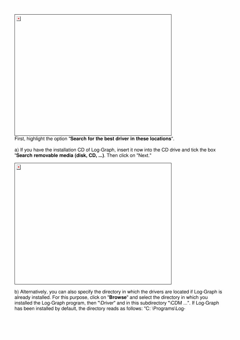
First, highlight the option "Search for the best driver in these locations". a) If you have the installation CD of Log-Graph, insert it now into the CD drive and tick the box "Search removable media (disk, CD, ...). Then click on "Next."

b) Alternatively, you can also specify the directory in which the drivers are located if Log-Graph is already installed. For this purpose, click on "Browse" and select the directory in which you installed the Log-Graph program, then "\Driver" and in this subdirectory "\CDM ...". If Log-Graph has been installed by default, the directory reads as follows: "C: \Programs\Log-

Graph\Driver\CDM... ". "\CDM... " corresponds to the driver version and could, for example, read as follows:" \CDM 2:02:04 WHQL Certified. Then click on "Next".

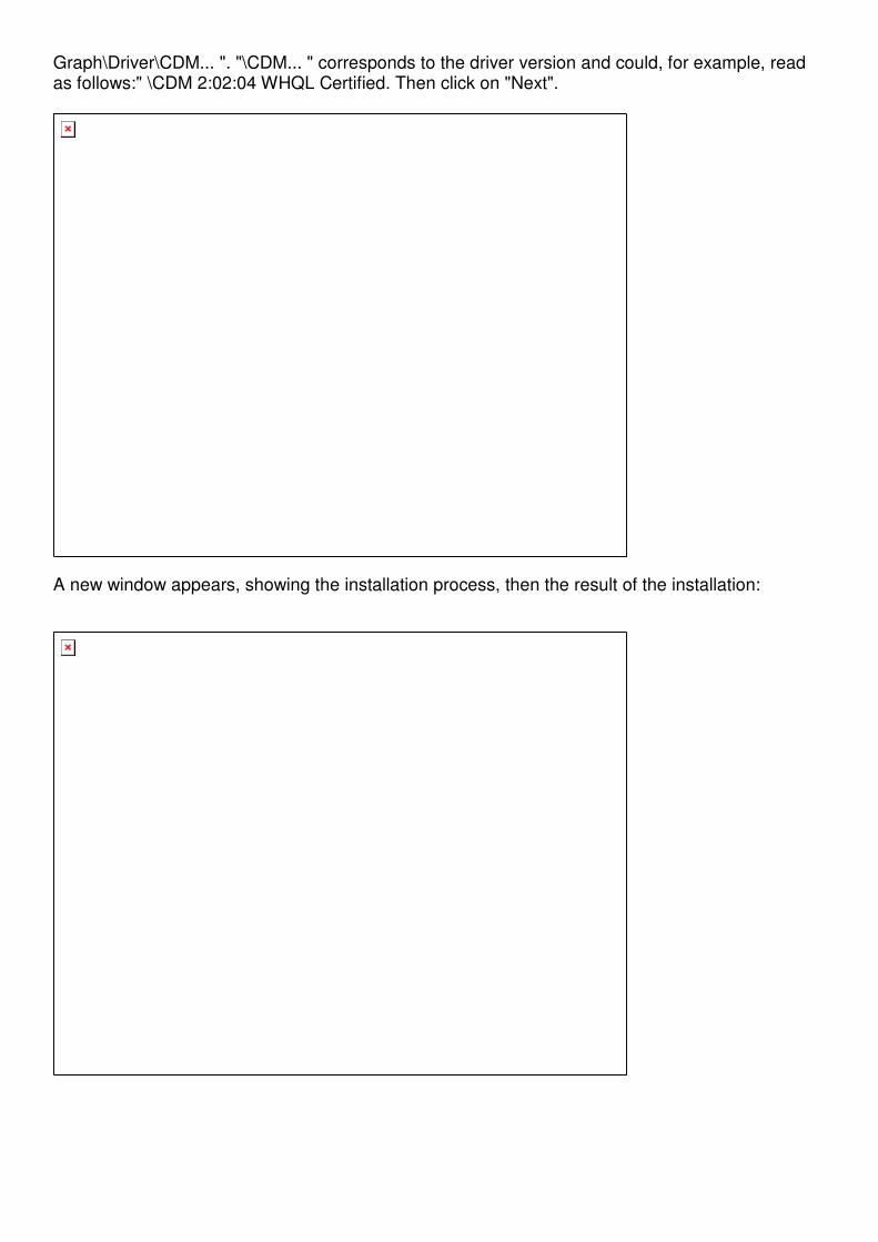
A new window appears, showing the installation process, then the result of the installation:

The device can now be used with the Log-Graph software. The name of a serial port (from COM1 to COM 256) has been automatically assigned to the USB port during the driver installation. Log-Graph automatically detects the assigned port. You can also find it under System settings where the port name can subsequently be changed. 2.7.3.2 Renaming the port

Usually, the automatically assigned port name does not need not be changed. However, if this is necessary, then you will find that name in "Device Manager" under "Ports (COM & LPT)". To get there, proceed as follows:

Click on "Start", then on "Control Panel". A new window appears:

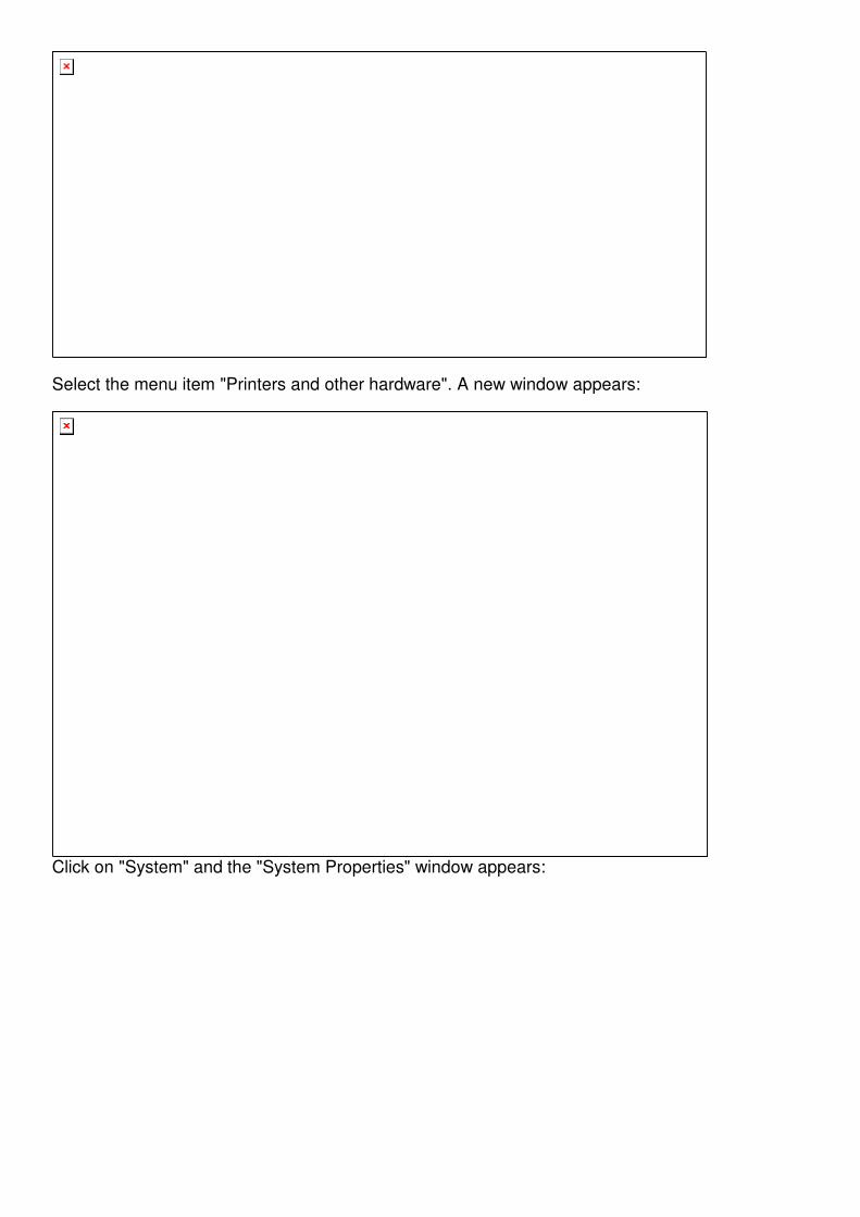
Select the menu item "Printers and other hardware". A new window appears:

Click on "System" and the "System Properties" window appears:

Select the "Hardware" tab.

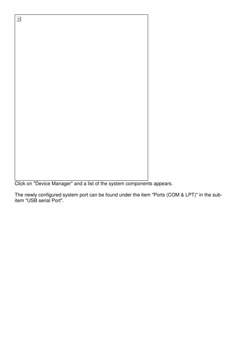
Click on "Device Manager" and a list of the system components appears. The newly configured system port can be found under the item "Ports (COM & LPT)" in the sub-item "USB serial Port".

Open the list by clicking on "Serial port". The relevant settings are displayed:

The system settings for the port can be found under the "Port settings" tab.

After clicking on "Advanced", the assigned port name (in this case COM4) is changed to another name (from COM1 to COM256). If you want to change it, please note that you can not use names that have already been assigned by the system. In the "COM port number" selection box, another assignment can be selected.

Click on "OK" to accept the settings and exit or "Cancel" to cancel the settings and exit. Then close all "Control Panel" windows you previously opened. The next time you start the Log-Graph software, you must register the logger under the newly assigned port number. To do so, enter manually the number under "Configure a port" or launch a search for the automatic detection of the port. a) Insert the CD into your drive and close the drive door. With most systems, the CD is automatically detected and the installation routine starts. If this is not the case, launch the installation via the taskbar by using the sequence Start-> Run-> [Your CD drive] -> Setup.exe.

b) Now, follow the instructions of the installation routine. During installation, a target directory Programs\Log-Graph that can be changed if necessary is proposed to you.

c) The installation process creates a program group for the selected directory on your PC and a program icon called "Log-Graph".

d) With a subsequent run, launch the program, for example, by double-clicking on the program icon "Log-Graph" on the desktop or by using the sequence Start-> Programs-> [Selection: Log-Graph] -> Mouse click.

e) In addition to the program "Log-Graph.exe", the online manuals, the help files and other files needed for setup are located on the CD.

3 Working with the Log-Graph software

This chapter describes the Log-Graph software structure and provides information about its operation. It is assumed that the user is familiar with the operation of a PC and the general functions of the Windows ® operating system.

Structure of the user interface

The software operation is performed either via the menu bar or via the toolbar. Selecting a menu item opens a new window in which the next software operation steps will be performed.

Menu bar:

Different groups of the program menu are located within the menu bar. After clicking on an option, the corresponding menu group opens and offers additional selection opportunities.

Toolbar:

The icons for frequently used functions are located within the toolbar. After clicking on an icon, the appropriate function is directly run without detour over the menu bar.

Online view:

The main data of an actually connected logger are displayed in Online Status on the left side of the screen.

Graph area:

The opened graphs and tables are displayed in the graph area on the right side.

Status line:

At the bottom of the window, a status line shows information about the ongoing operations of the program. The size of the window can be changed at will using the edges of the window frame and dragging them with the mouse. The "Minimize" box turns the window into an icon. "Maximize" expands the window to full screen size. "Close" allows you to quit the program (as for the menu item "File-> Quit").

User interface

The software operation is performed either via the menu bar or via the toolbar. Selecting a menu item opens a new window in which the next software operation steps will be performed.

3.1 Menu bar

The menu groups File, View, Logger, Graph, Window and Help are available for operation. The significance of the individual menu items is briefly described below:

3.1.1 Menu group File

Configure the logger port Searches for the logger on the available USB ports and defines its connection data Reactive the logger connection Tries to reactive an already used USB port National language Allows you to select and save the desired country settings Print (hardcopy) Prints a hardcopy of the currently displayed screen contents Quit Allows you to quit the program

3.1.2 Menu group View

Toolbar Shows or hides the toolbar in the top corner of the window Status bar Shows or hides the status bar in the bottom corner of the window Background Shows or hides the background image in the graph window

3.1.3 Menu group Logger

Logger setup (programming) opens a window for programming the logger Read out the data opens a window for reading out the recorded data Quick start of the logger starts the recording of the logger using the existing settings Quick stop of the logger stops the recording of the logger Set the time allows you to set the real- time clock in the logger Display the logger status opens a window that displays the current status of the logger Internal paramaters of the logger opens a window that displays all the available parameters of the logger (internal program

display)

3.1.5 Menu group Graph

As long as no graph is opened, only the menu item "Load the measurement file" is available.

Load the measurement file Loads an archived file

Once a graph is displayed, the following menu items are also available.

Fixed time axis Only displays the last xx minutes (adjustment under Manual graph settings) Graph and table Displays the graph and table values Graph Only displays the graph Tables Only displays the table values Load the measurement file Load an archived file

Copy Copies a graph to the clipboard as bitmap or metafile

Save as Saves a graph in one of the several graph formats Print Prints a copy of the currently displayed screen contents

Display the legend Shows or hides the legend in the graph

Horizontal grid lines Shows or hides the horizontal grid lines in the graph

Vertical grid lines Shows or hides the vertical grid lines in the graph 3D-three-dimensional Enables or disables the spatial graph view Zoom off Restores the inital size of the graph automatically X-axis Entering of minimum, maximum values or auto-scaling Y-axis Entering of minimum, maximum values or auto-scaling Graphical presentation Keyboard input for defining the graph

3.1.6 Menu group Window (window management)

The menu items are only available when multiple graphs are simultaneously opened (embedded windows) .

Arrange Arranges the windows in their order of appearance Cascade Stacks the windows on top of each other, while all remaining visible Horizontal tiling Arrange the windows one above the other (more rows than columns) Vertical tiling Arranges the windows side by side (more columns than rows) Minimize all Turns all windows into an icon Close all Closes all embedded windows

3.1.8 Menu group Help

Contents Help F1 Contents and index of all elements and terms used Log-Graph index Selection of the help topic via the search index Search by keyword Keyword collection and glossary General notes Opens a text editor for the creation of general notes about the program

Information about Log-Graph Brief information about the software

3.2 Toolbar (must be reviewed)

In the toolbar (quick start bar) at the top of the window below the menu bar, the frequently used functions can quickly be run without detour over the menu bar.

All the functions available there are also accessible from the menu bar via the pull-down menus.

3.3 Online view

The online view gives you the operating status of the logger. For this purpose, it is periodically verified at intervals of 1s whether a logger is connected, then the status of the logger is read and evaluated. � In standby mode, the connection is constantly monitored and the status is read once at the

beginning of the process. After that, the reading of non-modifiable status data is disabled. � In log mode, the connection is constantly monitored, and the status is read once at the beginning

of the process. Then, only the modifiable status data (the current record number and, if activated, the current measured values) are read. � In offline mode, it is not verified whether a logger is connected and the port is disabled. In this

case, only the display and evaluation functions are available under the menu item "Graphs".

The switchover between the online and offline mode is performed in the menu bar via the menu item "View -> Online status" or in the toolbar via the button "Online .

Logger in standby mode:

In Online view,

o the identifier of the logger,

o the operating mode (standby or log mode),

o the battery status,

o the logger time and

o the basic data related to the existing records

are always displayed.

In the upper free field, a customer-specific name can be entered.

The battery status indicator is updated only once per minute. Clicking on the battery status indicator or the menu item "View->Refresh the battery status" allows you to upload the value again.

Clicking on the clock icon next to the logger time allows you to synchronize the logger clock to a new setting (only in standby mode).

The operating mode (standby / log mode) is verified periodically at intervals of 1 s and provides additional information in log mode.

Logger in log mode:

In log mode, the online view provides as additional information

o the current record position and

o a table with the current measured values, the minimum and maximumvalues.

The table with the current values can be hidden, so reducing the data traffic on the port.

In continuous log mode , it is not possible to synchronize the logger clock to a new setting.

Software in offline mode:

If a logger is not connected (eg, with regard to the offline view for tables/graphs) or if the online view is not required, the latter can be enabled or disabled via the menu item "View-> Online status". In this case, no automatic status query can be performed and the currently connected logger will be ignored until the online view is activated again. Only functions that can be used "offline" are available, the online view is hidden, and only the graph area is displayed.

3.4 Graph area

All windows displaying graphs and/or tables of selected and archived data are embedded in the graph area. The archived files are opened via the menu item "Load the measurement file", and then displayed in the graph area in one or more windows.

Opening an archived file allows you to present its content as a table, a graph or a combination of both. The size of a newly opened window depends on the available graph area and uses by default about two thirds of the available width and two thirds of the available height. The size of each window can be tailored to your needs by dragging the edges with the mouse. Displaying the archived data in the graph area - one or more windows – allows you to manage the arrangement of these windows under the menu item "Window" (see 5.5 "Window management"). o "Minimize" turns the currently selected window into an icon,

o "Maximize" expands the currently selected window to the full size of the available graph area.

o The "Horizontal tiling" or "Vertical tiling" arrangement is only active with multiple windows. It

arranges the windows in rows (horizontal tiling) or columns (vertical tiling). The window size is adapted to the available graph area.

o "Stacked" or "Cascade" reduces all windows to the same size and shows the windows stacked

on top of each other, with the windows remaining visible.

o "Minimize all" turns all windows into an icon,

o "Close all" allows you to quit all windows in the graph area without any question (because no

data can be lost).

3.5 Status line

The status line at the bottom of the window contains information about the current program status or the current operations.

o The port used is specified in the first field,

o then follows the general status of the port in the second field and

o the currently performed operations are displayed in the third field The markings "T", "P", "R" and "W" under Mode in the third field and the background colour have the following meanings:

With regard to fields highlighted in grey , there is currently no operation, with regard to fields highlighted in green , the appropriately marked operation is taking place.

"R" and "W" represent the reading and writing operations during the communication with the logger.

"R" indicates a reading operation (Read, read out the data), "W" indicates a writing operation (Write, request the data), "T" indicates an operation that was automatically time-triggered (Timer) and "P" indicates an operation that was triggered by the program (Program).

Sometimes, time- and program-triggered communications may overlap. In this case, a short message appears and the newly requested operation will be executed once the previous one has been completed and the message has been confirmed. An automatic version which bypasses the message and even monitors the completion of the previous operation has not yet proved to be sufficiently safe, hence, until now, the use of the other method.

3.6 Basic settings for the software operation

The basic settings for the software operation are:

� the selected national language and � the port used for operation

The settings made are saved in the file .ini.

3.6.1 National language

When you launch the software for the first time (after the installation), the PC specifications for the national language are first accepted from the installation.

The national language may be selected independently of the system country settings. The changes only have an effect on the operation of the Log-Graph software and not on the system settings (or other programs). "Apply" saves the changes made in the file .ini. The changes are immediately effective and will be used by default during all subsequent program startups. "Cancel" undoes the changes made.

3.6.2 Configuring the port (must be reviewed)

For purposes of automatic detection, the new device to be installed must be connected via an appropriate cable and powered on and it must be the only device currently connected (the other devices that are already connected must be turned off). Enter all known values in order to shorten the time required for detection:

For "Connection to:" the number of the port (eg, Com 3) For "Transfer rate:" the baud rate set on the device

All ports available for connection are searched. Ports that are already used by a device or are being used by another program are not searched. Each verification (port, transfer rate) requires about 2 seconds. When a device that responds to the message is found, the search is interrupted and the settings found are saved in the device settings because of the information contained therein.

4.1 Starting the software

Start the software by double-clicking on the Log-Graph icon on the desktop or via the selection in the program manager with the sequence "Start-> Programs-> Log-Graph".

When the connection to the logger is successfully established, the following startup window appears shortly thereafter:

When you start the software, the program always searches for a connected logger. The following procedure is used: � The program checks whether a logger is on the port that was last configured (entry in the file .ini) � If the logger is not detected, an error message and a prompt appear. The latter asks you to

connect a logger, to search for other ports on which the logger could be configured or to use the software in offline mode. � After the selection of another port or a successful search, the port is checked again. � If the logger is detected, its status is read out and displayed in the online view. � The settings of the port available for use are saved in the file .ini for the next program startup. � When the program is launched for the first time, the USB port usually used for communication by

the device is not yet known and the program prompts you to configure the USB port (see "Configuring the logger port" ).

Once the connection is perfectly established, the current status of the connected logger appears on the left side in the online view.

In offline mode (if no logger is connected or the online view has been disabled), only the graph area in which archived files can be loaded and displayed is available. A return to the online view is done via the menu bar "View->Online status" or via the "Online" button in the toolbar when the logger is connected.

4.2 Programming the logger

The setup window for programming the logger is opened via the menu item "Logger-> Setup" or the shortcut key "Prog" in the toolbar. First, the operational readiness of the logger is checked and all the logger parameters required for programming are retrieved.

It takes a few seconds before all the data are uploaded and the setup window appears.

The parameters currently set in the logger are first displayed in the setup window. Many parameters can no longer be changed during the recording process, but they are only editable in standby mode. The appropriate entry positions are greyed out during the recording process and they are not usable.

The setup window contains four categories:

� Start/Stop/Measuring interval, � Limit values, � Display/Use and � Names

Load and Save:

"Load and Save" allows you to load the old logger settings and save the current logger settings under any file name with the default extension "Set". All settings, except the absolute start and stop time indications, can be reused for subsequent setups. When loading old settings, the logger time and the possible calibration values entered (subsequent, advanced option) are always preserved. Only the operating parameters for a new scheduled record are accepted from previous settings. A basic setting of the logger can also be restored in "Load". To this end, the file "\Settings\Default\ Default.set" must be loaded. It restores the initial status as described in the manual of the logger. Close

Close allows you to quit the programming. If changes have been made and they have not yet been transferred to the logger, a warning message appears. Transferring the settings

The settings made are sent to the logger and the setup window is closed. Only modifications are transferred. If no changes have been made, a corresponding message appears. If entries contain invalid data, the button stays greyed out until the corresponding corrections are made. After the transfer of settings, a corresponding response appears.

Start/Stop/Measuring interval:

The start and stop conditions correspond to those of the programming that was last performed. In general, these values are outdated because of the current logger time and they generate warning messages that possibly do not allow you to perform a save operation via the button "Transferring the settings". The start and stop time settings are checked while being entered and the results are displayed in the "Startup/Stop settings (Abstract) " area. If warning messages appear, transferring the settings is not possible and the "Transferring the settings" button is disabled. Startup settings:

The logger startup can be performed by simply pressing a button (start/stop button) or by using a Reed contact (option). This function can be disabled by unchecking the appropriate boxes. The other specifications allow: • the subsequent startup (using a button, Reed contact (optional) or PC command) • the immediate startup while transferring the new settings • the startup at a predefined time (date and time) When entering a start time, make sure that it is not less than the logger time or greater than the stop time. The start time should not be reached at the time when the data have completely been transferred to the logger, otherwise the program will not react to the entry of the start time. A verification only takes place during entry. To prevent the recorded data from being overwritten due to a restart occurred after pressing a button, the "Secure against multiple start" box can be activated. In this case, the logger can be restarted by simply pressing a button after the data have been read out, the setting via setup has been cancelled or the next startup is directly performed via software (with a previous overwrite warning).

Stop settings:

The logger stop can be performed by simply pressing a button (start/stop button) or by using a Reed contact (option). This function can be disabled by unchecking the appropriate boxes. The other specifications allow:

• the use of the internal memory as circular memory (the oldest records are overwritten when the memory is full)

• the stop as soon as the memory is completely filled (60,000 records)

• the stop at a preset time (date and time)

• the stop after a preset period *)

• the stop after a preset number of records *) The specifications marked with an asterisk *) limit the storage capacity to a record number less than 60000

When entering a stop time, make sure that it is not less than the logger time or less than the start time. The stop time should not be reached at the time when the data have completely been transferred to the logger, otherwise the program will not react to the entry of the stop time. A verification only takes place during entry.

Measuring interval:

The entry a measuring interval ranges from one second is to 86400 seconds and is presented in the format hours / minutes / seconds (hh: mm: ss). When 86400 seconds (24 hours) are reached, one day 00:00:00 appears. Just make sure that the measuring intervals do not exceed a value of approx. 3.5 hours with the planned and full utilization of the 60,000 records available since the lifetime of the battery would be reduced compared to the resulting lapse of time of nearly two years.

Limit values:

The minimum and maximum values can be predefined in the category "Limit values". The logger emits an alarm if the upper or lower limit values are exceeded.

Temperatures and humidity:

The limit values are available as lower limit (Lo) or upper limit (Hi) for each measuring channel. With LOG-100, these are only temperature limit values, With LOG-110, these are temperature and humidity limit values. An external sensor can only be used when the "Use an external sensor" box is activated. The entered limit values are only used when the corresponding boxes are activated. Whilst retaining the values, they may be easily activated or deactivated by simply modifying the boxes. Alarm output:

The treatment of the limit value surpassings can be performed via the red LED in the logger and / or the beeper. In the alarm output, the way of displaying messages is defined as well as the repetition rate of these messages and their display time. The repetition rates are limited to 64 seconds max. for the LED and beeper, the duration is limited to 10 s max. in increments of 0.5 seconds – each with a maximum duration of the lag set minus 0.5 s. A time lag of 0 second causes the deactivation of the alarm output. Alarm evaluation:

The alarm evaluation determines the delay time (in measurement cycles) with which the alarms must be treated, if they should occur in a cumulative way, if only the permanent alarms must be signalled and canceled. WARNING! The corresponding alarm messages only appear when the LED display or the beeper has not been disabled in the power saving options (Use the LED displays / Use the beeper).

Display/Use:

The general settings for the logger operation are summarized in the category Display/Use.

Logger time:

The date and time of the internal logger clock are displayed. After clicking on the "Set" button, you can synchronize the logger time in the "Set the logger date and time" window. While recording, it is not possible to modify the logger time.

Power saving functions and update intervals for LCD, LEDs and beeper:

Disabling the LCD display (it goes into sleep mode after pressing a button), deactivating the LED displays or the beeper reduce the power consumption of the logger and prolong the battery life.

LCD display:

During recording, the update of the logger display is performed at the pace of the measuring interval set. In standby mode, an update interval can be entered in the upper part of the display. When the "Use the sleep mode" box is activated, the LCD display goes into sleep mode after pressing the logger buttons and after expiration of the specified delay time. The logger no longer displays the measured values, but only a status ("run" during the recording process and "LC" in standby mode). When the "Off in sleep mode" box is activated, the status will no longer be displayed and the display will remain blank (until you use the buttons again).

LED displays green/red:

The LED displays are only used when the "Use the LED displays green/red" box is enabled. The green LED always flashes at the sample rate when the "Flash in green at the sample rate" option is activated. With regard to the red LED, a flashing (in addition to the settings made under Limit values) can be activated, if errors have occurred in the logger or arming occurs.

Beeper:

The beeper is only used when the "Use the beeper" option is activated. WARNING! The alarm messages specified in the category "Limit values" only appear when the LED display or the beeper has not been disabled in the power saving options (Use the LED displays / Use the beeper).

Temperature display:

The unit for the measurement display on the logger can be set to ° C or ° F.

Mode button:

The Mode button (switchover of the measurement display) can be locked against operation.

Names:

Up to eight names containing 16 characters max and any combination of characters can, for individual identification, be stored in the logger. The names are only loaded when that category is displayed.

Enter here any names that will allow you to clearly identify the logger.

4.3 Reading out the logger

The readout of recorded data is launched via the menu item "Logger->Read out the data" or the shortcut key "Read" in the toolbar. First, the operational readiness of the logger is checked and all the logger parameters required for programming are retrieved. It takes a few seconds before all the data are uploaded and the readout window appears.

The number of the available records, their start and stop time, the duration and the measuring interval set are displayed in the overview. Pressing the "Read out the Data" button causes the reading of the records to be started. In the lower part, the progress bar gives you an overview of the number of the already read records. It is possible to end prematurely the readout operation using the "Cancel ... " button. The already transferred records are completely undone (but they remain available in the logger and are not deleted). The readout can be performed again at a later date. After reading out the records, all the status information of the logger is also collected. After a successful readout, the records must be saved. The program proposes you a unique file name consisting of the date of the upload. This specification can be changed at will.

The file extension is always. dbf (a file compatible with dBase III). The status information is saved under the same name but with the extension. set. Press "Save" to save the files. After saving the records, the values can be displayed in graphical/tabular form.

For this purpose, click on "Display the graph". The data appear in a window of the graph area and can be further processed. "Close" allows you to quit the readout program.

4.4 Setting the logger time

The synchronization of the logger internal clock is performed via the menu item "Logger->Set the time" or the shortcut key "Time" in the toolbar. While recording, it is not possible to modify the logger time.

The window displays the current logger time and, for purposes of comparison, the current PC time. Depending on selection, o the PC time can directly be accepted or o set to any other value. Immediately after synchronization, there may be small deviations in the display of the PC clock and Logger clock (+/-1 second) due to delay in data transmission. "Transfer the date/time" allows you to set the logger time to the specified value.

4.5 Displaying the logger status

The status display of the current logger parameters is done via the menu item "Logger->Display the status" or the shortcut key "Stat" in the toolbar. First, the operational readiness of the logger is checked and all the logger parameters required for displaying the status are retrieved. It takes a few seconds before all the data are uploaded and the status window appears.

The categories "Hardware", "Status/Start/Stop" and "Alarms" contain information on the logger which was obtained by the same logger when recording (Status /Start/Stop), or which is invariably linked to the logger (hardware). During the recording process, some values may vary. Clicking on "Update" allows you to update the information contained in the currently displayed page. When "Read all ... " is highlighted, all status information is read again.

Hardware

Status/Start/Stop

Alarms/errors

4.6 Checking the operational readiness and reading all parameters

In the online view, only the most important data are transferred between the logger and the PC. Before executing the detailed tasks (programming, reading out the records, displaying the status, ...), the operational readiness of the logger is always checked and the complete set of parameters is always retrieved. The performed operations are displayed in the meantime.

In case of communication errors, appropriate hints are issued. It takes a few seconds before all the data are uploaded and the window of the detailed task called up appears.

4.7 Diagnostic functions

The display of all the current parameters available in the logger is done via the menu item "Logger->Diagnostic" or the shortcut key "Diag" in the toolbar. First, the operational readiness of the logger is checked and all the logger parameters required for displaying are retrieved. It takes a few seconds before all the data are uploaded and the display appears.

The data of the displayed page are updated using the button "Update". When "Read all ... " is highlighted, all parameters are read again and updated. This display is available for diagnostic purposes and is not intended for normal operation. That is why there is no detailed list of contents displayed. The display shows the memory area of important contents, arranged according to groups. The groups are combined according to data types. The mnemonics that are customary in the logger are used for identification, their names indicate their meaning.

ByteS and Boolean values BoolS1 and BoolS2

WordS, LongS and DataS

BlinkAndBeepS, StringS and IdnS

All data shown here are available in the appropriate program sections and are processed accordingly. The display of this original raw information is solely intended for diagnostic purposes in cases of functional checks.

5 Presentation of graphs and tables

As soon as the presentation of graph and/or table is opened, other processing points are available in the program menu. They are used to change the visualizations, to enter key values for presentation, and to export data or graphs from measurement tables. The presentation can be displayed in three different ways: • as pure graph (without table) • as combined presentation (graph and table) • as pure table (without graph)

When displaying a graph for the first time, the minimum and maximum values of the temperature and time axis and the scales in the ratio (grid lines) are automatically selected. On the left side, there are the temperature axis labels and at the bottom, the time axis labels. In the graph, the control elements for quick change of axis scalings are available on the left of the temperature axis, below the time axis. The minimum or maximum value shown is changed using the Up/Down button on the temperature axis or the Left/Right button on the time axis. In this case, the respective automatic axis scaling is disabled. The changes are always done in increments of the current grid line spacing. The automatic axis scaling of the respective minimum or maximum values of the axis is reactivated again using the automatic buttons Auto-up/-down or Auto-left /-right. If there is only one series of measurements, it is shown stretched over a period of 1 sec (otherwise the graph would appear empty because no single point is visible). Within the graph, the right and left mouse button can be used to change the image section (see 5.4.2 Process the graph views).

Graph and table

5.1 Graph and table

The presentation can be displayed either as a two-dimensional line graph or in 3D view. With regard to the 2D presentation the line widths can be changed. The table can optionally be displayed next to the graph or below the graph.

Minimum, maximum and average value

The minimum, maximum and average values of the recorded data are displayed next to the table (in 5.1.1) or above the table (for 5.1.2). These values are continuously updated during the acquisition process. When loading an existing file, these values are recalculated and displayed.

5.1.1 Graph and table side by side

The table is shown next to the graph. The table width always remains the same when changing the window size.

5.1.2 Table below graph

The table is shown below the graph. The table height is always about one-third of the total window height.

5.2 Graph (without table)

The presentation can be displayed either as a two-dimensional line graph or in 3D view. With regard to the 2D presentation the line widths can be changed.

5.3 Table (without graph)

All the measured values previously recorded are displayed in the table. The table always has the same structure. The arrangement and the number of table columns are the same for all devices, regardless of whether or not a device provides certain measured values. The front columns "Number", "Date" and "Time" are always used. The other columns can be filled with measured values, depending on the device used and the selected acquisition channels. The columns for which the connected device can not provide any value (eg the sensor is missing) remain empty.

Minimum, maximum and average value

The minimum, maximum and average values of the recorded data are displayed next to the table. These values are constantly updated during the acquisition process. When loading an existing file, these values are recalculated and displayed.

5.4 Functions for graph processing

A range of processing functions is available when displaying the graph. They are performed either via the menu group "Graph" in the main menu (see 3.2.4 menu group "Graph") or by using the toolbar in the header of the respective graph. The menu group uses the same icons as the toolbar.

The processing functions are available both during the processing of archived data (previously measured files) and when the graphs are displayed online during the acquisition process. With the graphs displayed online, the option "Update" can also be enabled – the graph and the table are respectively supplemented with the newest data at the acquisition interval pace.

5.4.1 Graph selection and settings

They are performed either via the menu group "Graph" in the main menu (see 3.2.4 menu group "Graph") or by using the toolbar in the header of the respective graph.

The menu group uses the same icons as the toolbar.

The menu group contains, in addition to the functions in the toolbar, the items "Copy", "Save as"

and "Load the measurement file".

The processing functions are available both during the processing of archived data (previously measured files) and when the graphs are displayed online during the acquisition process. With the graphs displayed online, the option "Update" can also be enabled – the graph and the table are respectively supplemented with the newest data at the acquisition interval pace. With a graph displayed online, this option is always automatically enabled as long as no section

appears or the automatic mode for the end of the time axis is disabled.

If the update has automatically been disabled by this kind of operation, this option can only be

reactivated by resetting and/or disabling the zoom function.

With the tables displayed online, the update is interrupted independently of the update of the

graph when if the table is browsed and when the newest line is not the last line shown in the table.

The update process continues when you go back to the last line at the table end.

Update automatically

This option is not available for the presentation of an already archived graph. However, with a graph displayed online, the newest value is always appended at the end of the time axis. If this is not desired, the automatic update can be deactivated. On the other hand, the enlargement of the graph section always causes the deactivation of the automatic update. If the automatic update is desired again, the option can be reactivated by clicking again on it.

Fixed time axis

Selecting the option "Fixed time axis" always causes the display of only one time interval – defined for a specific period of time – of the last measurement series. If this period is exceeded, the oldest measurement series escape left out of the graph while the new measurement series are appened to the right. The time interval displayed remains firmly stuck on the defined value. It can be modified under the item "Manual entries". The option can be disabled by simply clicking again on it. The automatic mode for time axis can be reactivated after confirmation.

Display the graph

Only displays the graph with the already recorded values and axis labels.

Graph and table side by side

Simultaneously displays the graph on the left side and the table on the right side.

Table below graph

Simultaneously displays the graph in the upper area and the table in the lower third.

Display the table

Only displays the table with the already recorded values.

Zoom to original size

The graph presentation is reset to its initial values. The automatic axis scaling is activated.

Zoom (+)

The graph presentation is enlarged to about 110% of its previous values. The automatic axis scaling is deactivated. If, because of this, the grid line spacing is less than 1 / 1000 ° C or less than 1 s, the presentation will be adapted to these minimum values.

Zoom (-)

The graph presentation is reduced to about 90% of its previous values. The automatic axis scaling is deactivated. If, because of this, the scalings of the original presentation are undershot, a further reduction will no longer be performed.

Manual entries

The minimum and maximum values of the temperature and time axes can manually be changed into arbitrary values via Manual entries. The subdivision of the grid lines (ticks) may vary and the line width for the 2D presentation can be set within a range of 1 to 10 pixels. If the presentation of a fixed time axis is selected, the maximum period shown in the graph is then defined.

View in 3D

The normal 2D line presentation is changed into a 3D presentation and vice versa.

Horizontal grid lines

The horizontal grid lines are shown or hidden.

Vertical grid lines

The vertical grid lines are shown or hidden.

Legend

The legend (description of the signal curves) on the upper or right edge of the graph is shown or hidden.

Print

"Print" starts printing the currently displayed graph section. You can choose between various options. The graph or table values are printed both individually and together.

5.4.2 Processing the graph views

Besides the selection of functions from the menu, some functions are directly carried out using the mouse. Some functions are activated using the left mouse button, others are activated using the right mouse button.

5.4.2.1 Selection using the left mouse button

While the left mouse button is pressed, a graph section can be selected for enlarged presentation or an already enlarged section will be restored to its original dimensions.

Enlarging the graph section

If, while holding down the left mouse button, you drag the mouse pointer from top left to bottom right, the graph is enlarged to the size of this area when you release the mouse button (with 3D view, the mouse pointer must be within the axis scales on the front plane, otherwise there will be no reaction). The automatic axis scaling is disabled.

Resetting the graph section

If, while holding down the left mouse button, you drag the mouse pointer from bottom right to top left - so unlike the procedure described above - the graph is reset to its original size when you release the mouse button. The automatic axis scaling is activated.

5.4.2.2 Selection using the right mouse button

While the right mouse button is pressed, the graph section shown can be moved to the left, right, up or down or reduced or enlarged in all four directions from the sides and angles. In this connection, the starting position on which you click with the right mouse button determines the next operation.

Depending on the starting position, the cursor changes its appearance and indicates the direction in which you can move. Five directions can be distinguished: - [1]. Left <> Right - [2]. Top <> Bottom - [3]. Bottom left <> Top right - [4]. Top left <> Bottom right - [5]. Move

[1] / [2] Reducing or enlarging the image section from the sides

If, while the right mouse button is pressed, the mouse is in a range from about 0-20% or 80% - 100% in the horizontal or vertical direction (almost in the middle of one of the graph edges), then the graph can be enlarged or reduced in the horizontal or vertical direction while holding down the mouse button. The automatic scaling of the concerned axes is deactivated.

The areas in which the mouse must be located for this purpose are hatched.

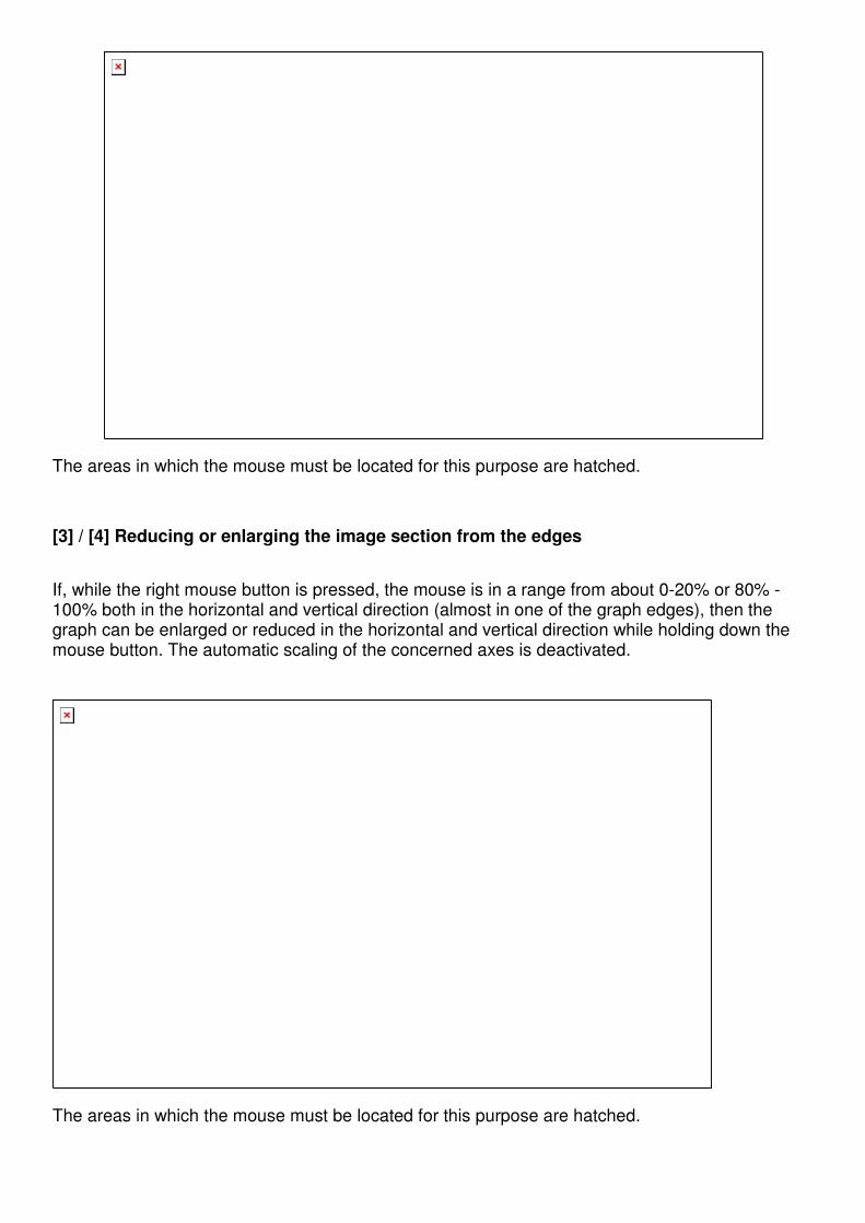
[3] / [4] Reducing or enlarging the image section from the edges

If, while the right mouse button is pressed, the mouse is in a range from about 0-20% or 80% - 100% both in the horizontal and vertical direction (almost in one of the graph edges), then the graph can be enlarged or reduced in the horizontal and vertical direction while holding down the mouse button. The automatic scaling of the concerned axes is deactivated.

The areas in which the mouse must be located for this purpose are hatched.

[5] Moving the image section:

If, while the right mouse button is pressed, the mouse is in a range from about 20% to 80% in the horizontal or vertical direction (almost in the middle of the graph area), then the graph can be moved in the horizontal or vertical direction while holding down the mouse button. The automatic axis scaling is deactivated.

The area in which the mouse must be located for this purpose is hatched. 5.4.3 Printing the graph and the records

The graph and the measurement series can be printed individually or together. The various possibilities can be selected as options.

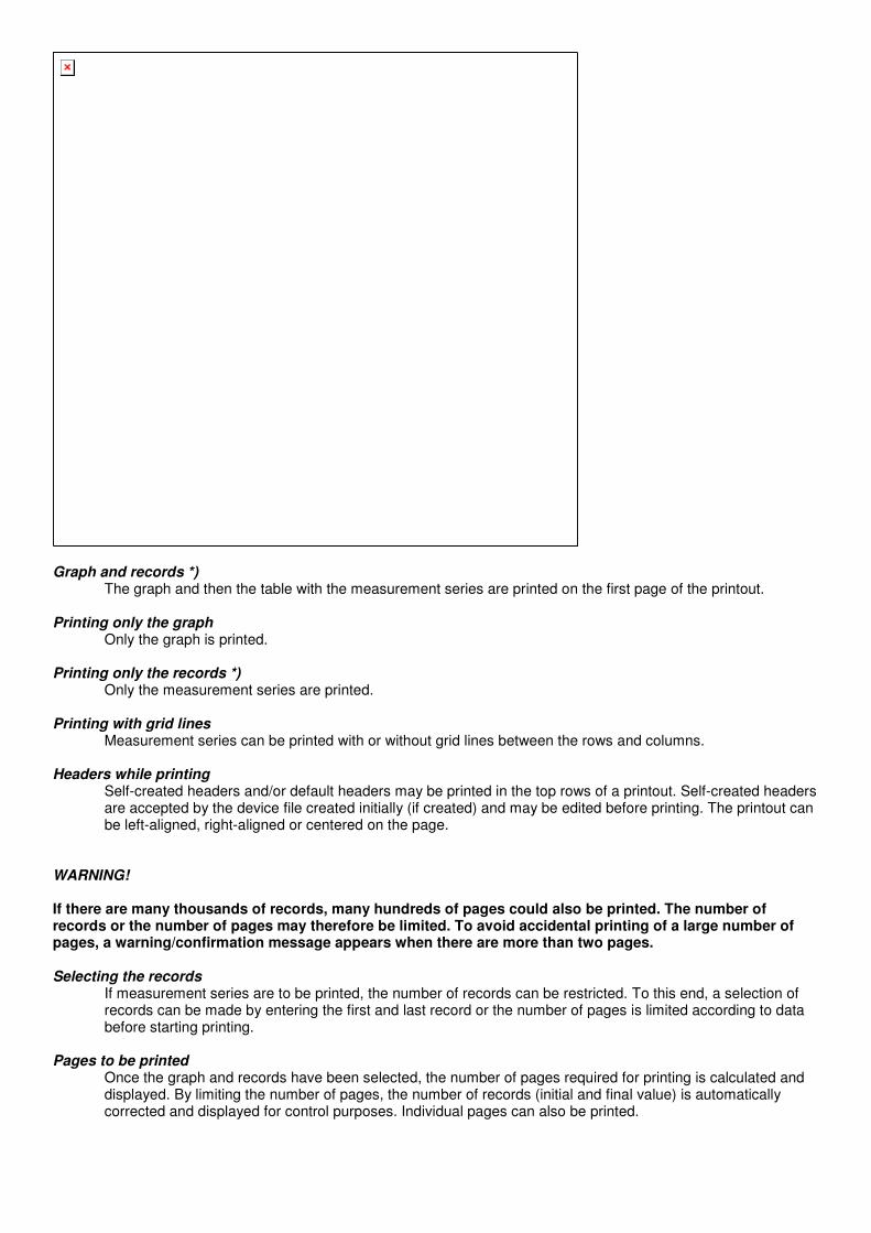
Graph and records *)

The graph and then the table with the measurement series are printed on the first page of the printout. Printing only the graph

Only the graph is printed. Printing only the records *)

Only the measurement series are printed. Printing with grid lines

Measurement series can be printed with or without grid lines between the rows and columns. Headers while printing

Self-created headers and/or default headers may be printed in the top rows of a printout. Self-created headers are accepted by the device file created initially (if created) and may be edited before printing. The printout can be left-aligned, right-aligned or centered on the page.

WARNING! If there are many thousands of records, many hundreds of pages could also be printed. The number of records or the number of pages may therefore be limited. To avoid accidental printing of a large number of pages, a warning/confirmation message appears when there are more than two pages. Selecting the records

If measurement series are to be printed, the number of records can be restricted. To this end, a selection of records can be made by entering the first and last record or the number of pages is limited according to data before starting printing.

Pages to be printed

Once the graph and records have been selected, the number of pages required for printing is calculated and displayed. By limiting the number of pages, the number of records (initial and final value) is automatically corrected and displayed for control purposes. Individual pages can also be printed.

Configure

With "Configure", the options available on the printer may be adapted to printing. These are, eg, the paper size (portrait / landscape), the printer resolution and quality or the number of copies. The options available depend on the capabilities of the printer driver installed. However, it is possible that all the capabilities of your printer driver are not used when printing via Log-Graph.

Print

"Print" allows you to start printing using the settings previously made. If there are more than two pages, a security question appears asking you if you really want to print the page number indicated.

Cancel

" Cancel" allows you to quit the print dialog and return to the starting point without any further operation.

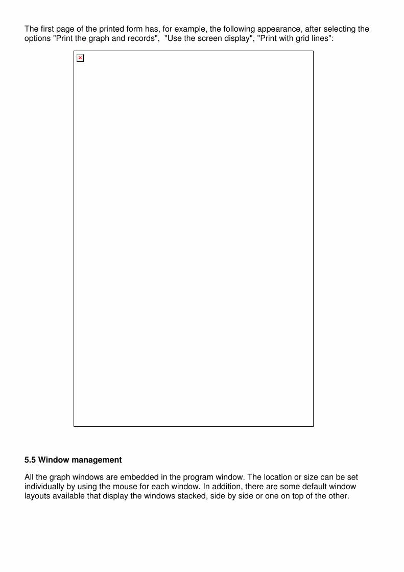
The first page of the printed form has, for example, the following appearance, after selecting the options "Print the graph and records", "Use the screen display", "Print with grid lines":

5.5 Window management

All the graph windows are embedded in the program window. The location or size can be set individually by using the mouse for each window. In addition, there are some default window layouts available that display the windows stacked, side by side or one on top of the other.

Cascade presentation

The windows are displayed stacked upon each other while all remain visible. This arrangement is particularly useful when there is a larger number of windows, because you can bring the desired window to the foreground – whilst the size remains unchanged - after clicking on the window title.

There are also two other arrangement patterns: vertical tiling and horizontal tiling. In both cases the window division is carried out in such a way that all windows are simultaneously displayed and their size is adjusted to the space available. If there is a small number of windows, they are arranged in a row (vertical tiling) or in a column (horizontal tiling). If there is a larger number of windows, several rows and columns are used for display. With vertical tiling, you use more columns than rows, and with horizontal tiling, more rows than columns. If you select "Minimize all windows", all windows are minimized and arranged as icons at the bottom of the screen. If you select "Close", the active window is closed. If you select "All windows", all windows are simultaneously closed.

Horizontal tile presentation

Vertical tile presentation

6 Log-Graph editor (must be reviewed)

The editor integrated in Log-Graph allows you to enter notes on an application or a measurement file and to open (plain) text files in a similar way to MicroSoft ® NotePad

The functions generally available are Open, Save and Print a file, Paste, Copy or Cut a text for the connection to other applications via the clipboard. When you click on the editor icon in the Log-Graph environment, an automatic file name referring to the environment is always assigned. With measurement files, the name of the measurement file is automatically used and is given the extension ".txt" (eg for a file Pro12_20040723-1.dbf the name Pro12_20040723-1.txt ). The general notes which are created under the menu item "Help" in the main program will automatically receive the name "Log-Graph.txt". The automatic naming is designed to facilitate the assignment. Of course, the files can also be stored under different names. When you click on the editor icon, Log-Graph always searches for the already existing files with the automatically assigned name mapping. The renamed files must always be explicitly loaded using the menu item "File-> Open".

6.1 Special functions of the Log-Graph editor in the active graph window

If the editor related to a measurement file is opened, other automated functions which allow you to append the current program settings or device parameters from the program are available. In addition to manual entries, other current data can be added via the selection. For this purpose, after pressing the "Parameters" button or in the menu "Edit->Insert default parameters", a selection of the available data is displayed. The available data correspond to the settings that were used in the logger at the time of acquisition. They include, for example, the start and stop time, the measuring interval set, the device IDs, ... Therefore, all the parameters set in the logger can easily be added to the documentation.

The selected information is always added at the end of the text. From there, they can be moved to any other locations via Cut or Copy. The selection of the available parameters can be made individually or if you click on the "Insert all" button, all information in the block will be appended to the existing text.

The caption on the buttons shows the categories for which the information is availabe. To determine the type of information that will be entered in detail using the respective selection, launch the editor, click once on each of the selection buttons at the top and watch the type of information that will be added to the text. To use the device parameters available only here elsewhere, first download the parameters using the selection buttons at the top of the editor and copy the desired lines into any other formats via the clipboard.

7 Annex (must be reviewed)

In the annex, there are the tables for memory requirements and recording times as well as the version overview. Version overview

Version overview (newest versions always on the top) Version 1.0.1 (ended on xx.05.2010)

• Version 1.0.1 First release version (as in the specifications)