Embed Size (px)
Citation preview
1
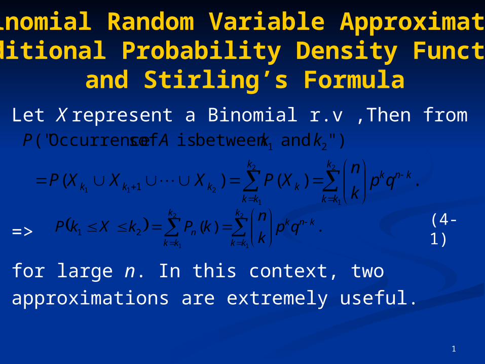
Let X represent a Binomial r.v ,Then from
=>
for large n. In this context, two approximations are
extremely useful.
2
1
2
1
.)(21
k
kk
knkk
kkn qp
k
nkPkXkP (4-1)
4. Binomial Random Variable Approximations,Conditional Probability Density Functions
and Stirling’s Formula
.)()(
) " and between is of sOccurrence ("
2
1
2
1
211 1
21
k
kk
knkk
kkkkkk qp
k
nXPXXXP
kkAP

2
4.1 The Normal Approximation (Demoivre-Laplace Theorem)
Suppose with Suppose with pp held fixed. Then for held fixed. Then for kk in the in the neighborhood of neighborhood of npnp, we can approximate , we can approximate
And we have:And we have:
wherewhere
n
npq
.2
1 2/)( 2 npqnpkknk enpq
qpk
n
,2
1
2
1 2/
2/)(
21
22
1
22
1
dyedxenpq
kXkP yx
x
npqnpxk
k
(4-2)
(4-3)
. , 22
11
npq
npkx
npq
npkx

3
(4-2).2
1 2/)( 2 npqnpkknk enpq
qpk
n
Thus if and in (4-1) are within or around the neighborhood of the interval we can approximate the summation in (4-1) by an integration. In that case (4-1) reduces to
where
We can express (4-3) in terms of the normalized integral
that has been tabulated extensively (See Table 4.1).
1k 2k
, , npqnpnpqnp
,2
1
2
1 2/
2/)(
21
22
1
22
1
dyedxenpq
kXkP yx
x
npqnpxk
k
(4-3)
)(2
1)(
0
2/2
xerfdyexerfx y
(4-4)
. , 22
11
npq
npkx
npq
npkx

4
x erf(x) x erf(x) x erf(x) x erf(x)
0.050.100.150.200.25
0.300.350.400.450.50
0.550.600.650.700.75
0.019940.039830.059620.079260.09871
0.117910.136830.155420.173640.19146
0.208840.225750.242150.258040.27337
0.800.850.900.951.00
1.051.101.151.201.25
1.301.351.401.451.50
0.288140.302340.315940.328940.34134
0.353140.364330.374930.384930.39435
0.403200.411490.419240.426470.43319
1.551.601.651.701.75
1.801.851.901.952.00
2.052.102.152.202.25
0.439430.445200.450530.455430.45994
0.464070.467840.471280.474410.47726
0.479820.482140.484220.486100.48778
2.302.352.402.452.50
2.552.602.652.702.75
2.802.852.902.953.00
0.489280.490610.491800.492860.49379
0.494610.495340.495970.496530.49702
0.497440.497810.498130.498410.49865
Table 4.1

5
Example 4.1
A fair coin is tossed 5,000 times. Find the A fair coin is tossed 5,000 times. Find the probability that the number of heads is probability that the number of heads is between 2,475 to 2,525.between 2,475 to 2,525.
Solution:Solution: We need We need Here Here nn is large so that we can use the is large so that we can use the normal approximation. In this case normal approximation. In this case so that and so that and Since andSince and
the approximation is valid for andthe approximation is valid for and
).525,2475,2( XP
,2
1p 500,2np .35npq
,465,2 npqnp
475,21 k .525,22 k
,535,2 npqnp

6
Example 4.1(cont.)
Here
From table(4-1):
2
1
2
.2
1 2/21
x
x
y dyekXkP
.7
5 ,
7
5 22
11
npq
npkx
npq
npkx
,516.07
5erf2
|)(|erf)(erf)(erf)(erf525,2475,2 1212
xxxxXP
. 258.0)7.0(erf
7
4.2. The Poisson Approximation
for large n, the Gaussian approximation of a binomial
r.v is valid only if p is fixed, i.e., only if and
what if is small, or if it does not increase
with n?
for example, as such that is a
fixed number.
1np
.1npq np
0p ,n np
8
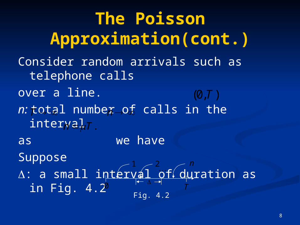
The Poisson Approximation(cont.)
Consider random arrivals such as telephone calls
over a line.n: total number of calls in the interval as we haveSuppose : a small interval of duration as in Fig. 4.2
).,0( T
T n
.Tn
0 T
Fig. 4.2
1 2 n

9
The Poisson Approximation(cont.)
p: probability of single call occurring in . as
=>normal approximation is invalid here.Suppose the interval in Fig. 4.2:(H) “success” : : A call inside ,(T ) “failure” : : A call outside : probability of obtaining k calls (in
any order) in an interval of duration , ,
.T
p
0p .T
T
Tnp
)(kPn
knkn pp
kkn
nkP
)1(
!)!(
!)(

10
The Poisson Approximation(cont.)
rewrite (4-6) as:
The right side of (4-8) represents the Poisson p.m.f.
.)/1(
)/1(
!
11
21
11
)/1(!
)()1()1()(
k
nk
knk
kn
n
n
kn
k
nn
nnpk
np
n
knnnkP
Thus ,!
)(lim ,0 ,
e
kkP
k
nnppn
(4-7)
(4-8)

11
Example 4.2
Winning a Lottery:
Suppose two million lottery tickets are issued with 100 winning tickets among them.
(a) If a person purchases 100 tickets, what is the probability of
winning?
(b) How many tickets should one buy to be 95% confident of having a winning ticket?
Solution:P:The probability of buying a winning ticket
.105102
100
ticketsof no. Total
tickets winningof No. 56
p

12
Example 4.2(cont.)
X: number of winning tickets n: number of purchased tickets , ,
P: P: an approximate Poisson distribution with parameter
,100n
.005.0105100 5 np
,!
)(k
ekXPk
13
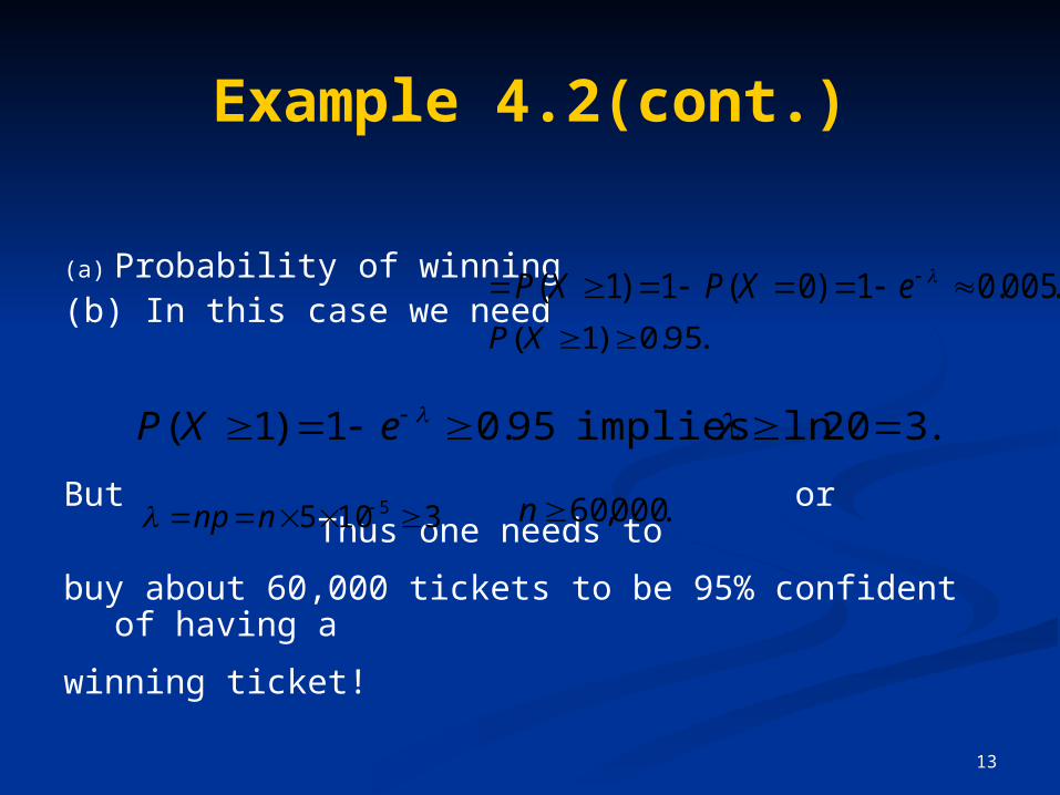
Example 4.2(cont.)
(a) Probability of winning (b) In this case we need
But or Thus one needs to
buy about 60,000 tickets to be 95% confident of having a
winning ticket!
.005.01)0(1)1( eXPXP
.95.0)1( XP
.320ln implies 95.01)1( eXP
3105 5 nnp .000,60n

14
Example 4.3
A space craft has 100,000 components The probability of any one component being defective is The mission will be in danger if five
or more components become defective. Find the
probability of such an event.Solution: n is large and p is small => Poisson approximation is valid with parameter
n
).0(102 5 p
,2102000,100 5 np

15
Example 4.3(cont.)
.052.03
2
3
42211
!1
!1)4(1)5(
2
4
0
24
0
e
ke
keXPXP
k
kk
k

16
Conditional Probability Density Function
, )( )( xXPxFX
.0)( ,)(
)()|(
BP
BP
BAPBAP
.
)(
)( |)( )|(
BP
BxXPBxXPBxFX
(4-9)
(4-10)
(4-11)
.0
)(
)(
)(
)( )|(
,1)(
)(
)(
)( )|(
BP
P
BP
BXPBF
BP
BP
BP
BXPBF
X
X
(4-12)

17
Conditional Probability Density Function
Further
Since for
),|()|(
)(
)( )|)((
12
2121
BxFBxF
BP
BxXxPBxXxP
XX
,12 xx
. )()()( 2112 xXxxXxX
(4-13)
(4-15)
(4-14)
,
)|()|(
dx
BxdFBxf X
X
(4-16)
2
1
21 .)|(|)(x
x X dxBxfBxXxP
x
XX duBufBxF
.)|()|(
(4-17)
18
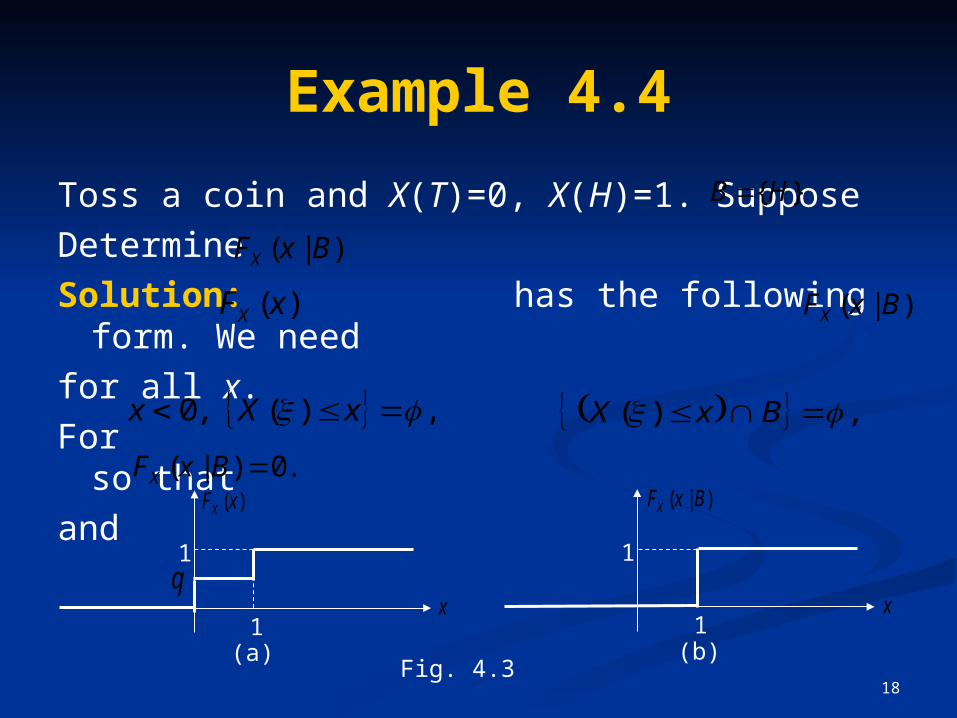
Example 4.4
Toss a coin and X(T)=0, X(H)=1. Suppose Determine Solution: has the following form.
We needfor all x. For so thatand
}.{HB
).|( BxFX
)(xFX )|( BxFX
,)( ,0 xXx ,)( BxX
.0)|( BxFX
)(xFX
x
(a)
q1
1
( | )XF x B
x
(b)
1
1
Fig. 4.3

19
Example 4.4(cont.)
For so that
For and
(see Fig. 4.3(b)).
, )( ,10 TxXx
HTBxX )( .0)|( and BxFX
,)( ,1 xXx
}{ )( BBBxX 1)(
)()|( and
BP
BPBxFX

20
Example 4.5
Given suppose Find
Solution: We will first determine From (4-11)
and B as given above, we have
For so that
),(xFX .)( aXB ).|( Bxf X
).|( BxFX
.
)|(
aXP
aXxXPBxFX
(4-18)
xXaXxXax ,
.
)(
)()|(
aF
xF
aXP
xXPBxF
X
XX
(4-19)
21
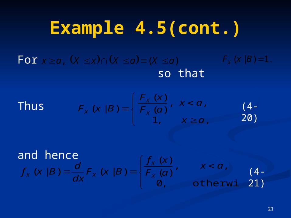
Example 4.5(cont.)
For so that
Thus
and hence
)( , aXaXxXax .1)|( BxFX
, ,1
, ,)(
)()|(
ax
axaF
xFBxF
X
X
X(4-20)
otherwise. ,0
,,)(
)()|()|(
axaF
xfBxF
dx
dBxf
X
X
XX (4-21)

22
Example 4.5(cont.)
)|( BxFX
)(xFX
xa
1
(a)
)|( Bxf X
)(xf X
xa(b)
Fig. 4.4

23
Example 4.6
Let B represent the event withFor a given determine and
Solution:
bXa )( .ab
),(xFX )|( BxFX ).|( Bxf X
.
)()(
)( )(
)(
)()( |)( )|(
aFbF
bXaxXP
bXaP
bXaxXPBxXPBxF
XX
X

24
Example 4.6(cont.)For we have
and hence
For we haveand hence
For we haveso that
,bxa })({ )( )( xXabXaxX
.
)()(
)()(
)()(
)()|(
aFbF
aFxF
aFbF
xXaPBxF
XX
XX
XXX
(4-24)
,bx bXabXaxX )( )( )(
.1)|( BxFX (4-25)
,ax ,)( )( bXaxX
.0)|( BxFX (4-23)

25
Example 4.6(cont.)Using (4-23)-(4-25), we get (see Fig.
4.5)
otherwise.,0
,,)()(
)()|(
bxaaFbF
xfBxf
XX
X
X
)|( Bxf X
)(xf X
x
Fig. 4.5
a b

26
Conditional p.d.f & Bayes’ theorem
First, we extend the conditional probability results to random variables:
We know from chapter 2 (2-41) that:
If is a partition of S
and B is an arbitrary event, then:
)()|()()|()( 11 nn APABPAPABPBP
)],,,[ 21 nAAAU

27
Conditional p.d.f & Bayes’ theorem
1. Setting in (2-41) we obtain
Son partition a form ,
)()|()()|()(
)()|()()|()(
Hence
)()|()()|()(
1
11
11
11
n
nn
nn
nn
AA
APAxfAPAxfxf
APAxFAPAxFxF
APAxXPAPAxXPxXP
}{ xXB

28
conditional p.d.f& Bayes’ theorem
2. From the identity
It follows that:
.)(
)()|()|(
BP
APABPBAP
)(
|
)(|
)|
APxF
AxF
APxXP
AxXPxXAP
(4-26)

29
Conditional p.d.f & Bayes’ theorem
3. Setting in (4-27) we conclude that:
(4-27)
21 )( xXxB
).()(
)|()(
)()(
)|()|(
)(|
|
2
1
2
1
12
12
21
2121
APdxxf
dxAxfAP
xFxF
AxFAxF
APxXxP
AxXxPxXxAP
x
x X
x
x X
XX
XX
(4-28)
30
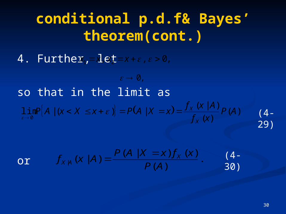
conditional p.d.f& Bayes’ theorem(cont.)
4. Further, let
so that in the limit as
or
,0 , , 21 xxxx
,0
).()(
)|(|)(|lim
0AP
xf
AxfxXAPxXxAP
X
X
(4-29)
.)(
)()|()|(| AP
xfxXAPAxf X
AX
(4-30)

31
conditional p.d.f& Bayes’ theorem(cont.)
Total probability theorem.From (4-30), we also get
or
,)()|()|()(
1
dxxfxXAPdxAxfAP XX
(4-31)
dxxfxXAPAP X )()|()(
(4-32)

32
Conditional p.d.f & Bayes’ theorem
Bayes’ theorem.using (4-32) in (4-30), we get the desired
result
.)()|(
)()|()|(|
dxxfxXAP
xfxXAPAxf
X
XAX (4-33)

33
Example 4.7
Reexamine the coin tossing problem: : probability of obtaining a head in a toss.For a given coin, a-priori p can possess any value in the interval (0,1). In the absence of any additional
information, we may assume the a-priori p.d.f to be a uniform distribution in that interval. Now suppose we actually perform an experiment of tossing the coin n times, and
k heads are observed. This is new information. How can
we update
)(HPp
)( pfP
?)( pfP
34
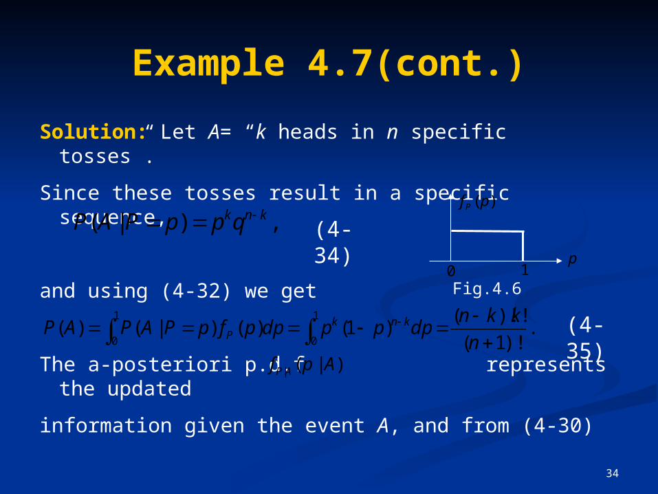
Example 4.7(cont.)
Solution: Let A= “k heads in n specific tosses”.
Since these tosses result in a specific sequence,
and using (4-32) we get
The a-posteriori p.d.f represents the updated
information given the event A, and from (4-30)
,)|( knkqppPAP (4-34)
)( pfP
p0 1
Fig.4.6
.)!1(
!)!()1()()|()(
1
0
1
0
n
kkndpppdppfpPAPAP knk
P(4-35)
| ( | )P Af p A

35
Example 4.7(cont.)
Notice that the a-posteriori p.d.f of p in (4-36) is not a uniform
distribution, but a beta distribution. We can use this a-posteriori
p.d.f to make further predictions, For example, in the light of the
above experiment, what can we say about the probability of a head
occurring in the next (n+1)th toss?
).,( 10 ,!)!(
)!1(
)(
)()|()|(|
knpqpkkn
n
AP
pfpPAPApf
knk
PAP
)|(| Apf AP
p
Fig. 4.7
10
(4-36)

36
Example 4.7(cont.)
Let B= “head occurring in the (n+1)th toss, given
that k heads have occurred in n previous tosses”.
Clearly and from (4-32)
Thus, if n =10, and k = 6, then
which is more realistic compare to p = 0.5.
,)|( ppPBP
1
0 .)|()|()( dpApfpPBPBP P (4-38)
,58.012
7)( BP


![INSTITUTE OF MATHEMATICS HEBREW …arXiv:1206.0153v2 [q-fin.CP] 17 Oct 2013 ERROR ESTIMATES FOR BINOMIAL APPROXIMATIONS OF GAME PUT OPTIONS YONATAN IRON AND YURI KIFER INSTITUTE OF](https://img.pdfslide.us/doc/110x75/5ea704863bc4c2796711adc1/institute-of-mathematics-hebrew-arxiv12060153v2-q-fincp-17-oct-2013-error-estimates.jpg)