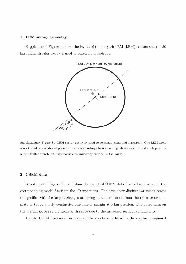
1. LEM survey geometry

Supplemental Figure 1 shows the layout of the long-wire EM (LEM) sensors and the 30

km radius circular towpath used to constrain anisotropy.

LEM 1 at 51º

LEM 2 at -39º

Anisotropy Tow Path (30 km radius)

Main CSEM

Tow Line

Supplementary Figure S1: LEM survey geometry used to constrain azimuthal anisotropy. One LEM circle

was situated on the abyssal plain to constrain anisotropy before faulting while a second LEM circle position

on the faulted trench outer rise constrains anisotropy created by the faults.

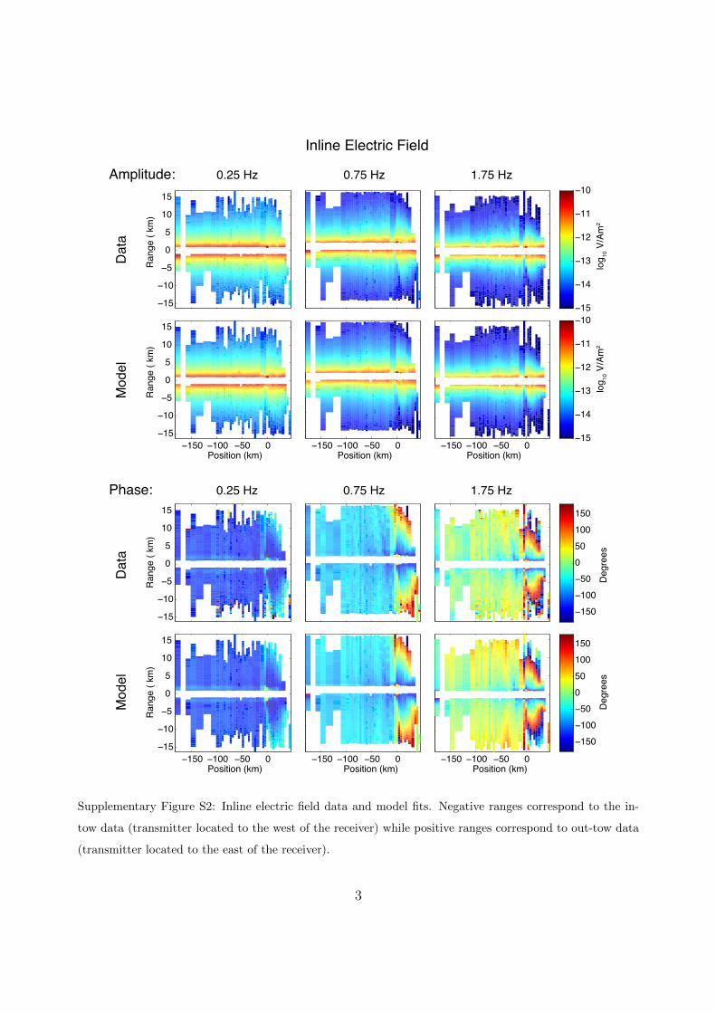
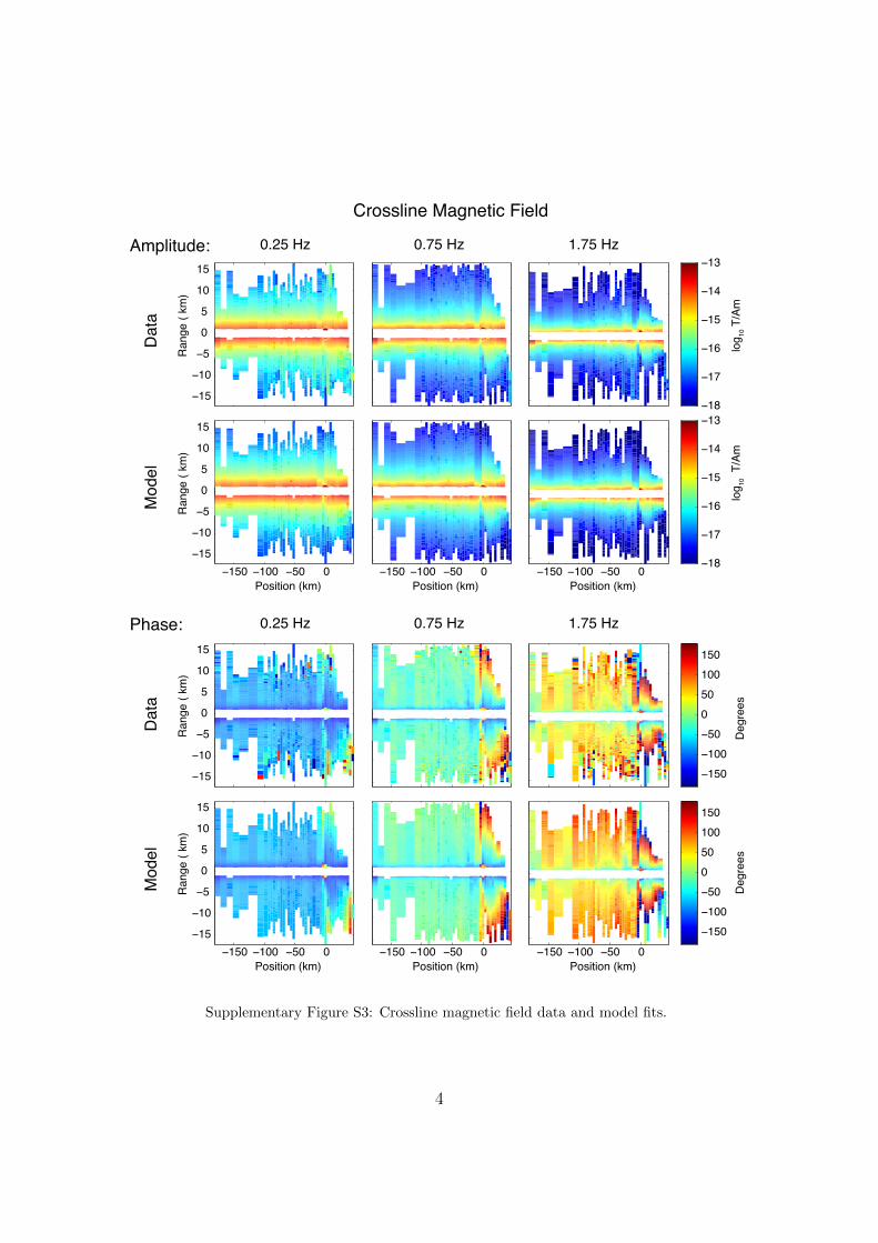
2. CSEM data

Supplemental Figures 2 and 3 show the standard CSEM data from all receivers and the

corresponding model fits from the 1D inversions. The data show distinct variations across

the profile, with the largest changes occurring at the transition from the resistive oceanic

plate to the relatively conductive continental margin at 0 km position. The phase data on

the margin slope rapidly decay with range due to the increased seafloor conductivity.

For the CSEM inversions, we measure the goodness of fit using the root-mean-squared

1

(RMS) error:

RMS =

√√√√ 1

n

n∑i=1

[di −mi

si

]2, (1)

where n is the number of data, si is the standard error of the ith datum di (i.e. an electric

or magnetic field at a given frequency, receiver and transmitter location) and mi is the

corresponding model response.

2

−15

−10

−5

0

5

10

15

Ran

ge (

km)

−150 −100 −50 0−15

−10

−5

0

5

10

15

Position (km)

Ran

ge (

km)

Dat

aM

odel

D

ata

Mod

el

−15

−10

−5

0

5

10

15

Ran

ge (

km)

−150 −100 −50 0−15

−10

−5

0

5

10

15

Position (km)

Ran

ge (

km)

−150 −100 −50 0Position (km)

−150 −100 −50 0Position (km)

−150 −100 −50 0Position (km)

−150 −100 −50 0Position (km)

−15

−14

−13

−12

−11

−10

−15

−14

−13

−12

−11

−10

−150−100−50050100150

−150−100−50050100150

0.25 HzAmplitude:

Phase:

Inline Electric Field

0.75 Hz 1.75 Hz

log 10

V/A

m2

Deg

rees

Deg

rees

log 10

V/A

m2

0.25 Hz 0.75 Hz 1.75 Hz

Supplementary Figure S2: Inline electric field data and model fits. Negative ranges correspond to the in-

tow data (transmitter located to the west of the receiver) while positive ranges correspond to out-tow data

(transmitter located to the east of the receiver).

3

−15

−10

−5

0

5

10

15

Ran

ge (

km)

−150 −100 −50 0−15

−10

−5

0

5

10

15

Ran

ge (

km)

Position (km)

−15

−10

−5

0

5

10

15

Ran

ge (

km)

−150 −100 −50 0−15

−10

−5

0

5

10

15

Ran

ge (

km)

Position (km)

−150 −100 −50 0Position (km)

−150 −100 −50 0Position (km)

−150 −100 −50 0Position (km)

−150 −100 −50 0Position (km)

−18

−17

−16

−15

−14

−13

−18

−17

−16

−15

−14

−13

−150−100−50050100150

−150−100−50050100150

Dat

aM

odel

D

ata

Mod

el

0.25 HzAmplitude:

Phase:

Crossline Magnetic Field

0.75 Hz 1.75 Hz

0.25 Hz 0.75 Hz 1.75 Hz

log 10

T/A

mD

egre

esD

egre

eslo

g 10 T

/Am

Supplementary Figure S3: Crossline magnetic field data and model fits.

4