1

Lecture 4Lecture 41. Statistical-mechanical approach to dielectric

theory.

2. Kirkwood-Fröhlich's equation.

3. The Kirkwood correlation factor.

4. Applications: pure dipole liquids, mixtures, dipolar solids.

2

The methods of statistical mechanics provide a way of obtaining macroscopic quantities when the properties of the molecules and the molecular interactions are known.

All statistical-mechanical theories of the dielectric constant start from the consideration that the polarization PP, given by:

ΕDP4is equal to the dipole density P, , when the influence of higher when the influence of higher multipole densities may be neglectedmultipole densities may be neglected. By definition, we may write the dipole density PP of a homogeneous system:

MPV (4.1)

where V V is the volume of the dielectric under consideration an <<MM>> is its average total (dipole) moment (the brackets < > denote a statistical mechanical average). If we assume the system to be isotropic, we also have

ED

3

Thus we find:

M=EV

41 (4.2)

Since the dielectric is isotropic, <M<M>> will have the same direction as E E and it will be sufficient to calculate the average component of M M in the direction of EE.. Using ee to denote a unit vector in the direction of the field, we may therefore rewrite Eqn (4.2) in scalar form:

eMeM= VV

E 44

1 (4.3)

Another way of writing Eqn.(4.3) results form the fact that PP and <<MM>> contain in general also terms in higher powers of EE than the first (see eqn.(1.19)). Thus, ((-1)E/4-1)E/4 is the first term in a series development of PP in powers of EE, and must be set equal to the term linear in EE of the series development of <<MMee>/>/VV in powers of EE.. Since variations in VV due to electrostriction do not appear in the leaner term we may develop <<MMee>> in a Taylor series, finding:

0

41

EEVeM=

4

Rewriting with the external field EEoo instead of the Maxwell field Maxwell field EE as the independent variable we obtain:

(4.4)

14 0

0 0 00

= M eV

E

E EE E

For the average of a quantity like MMee, which is a function of the positions and orientations of all molecules, one can write:

M eM e

dX U kT

dX U kT

exp( / )

exp( / )(4.5)

where XX denotes the set of position and orientation variables of all molecules. This expression for the average can be obtained from the general ensemble average by integrating over the momenta. The integration over the moment results in a weight factor, which is contained in our notation dXdX. For example, if we take spherical coordinates r,r,,, for the position of a molecule and integrate over the conjugated momenta, we obtain a weight factor rr22sinsin,, in this integration over the coordinates of that molecule. Thus, in this case dX=rdX=r22sinsindrddrddd,, which is the expression for a volume element in spherical coordinates.

5

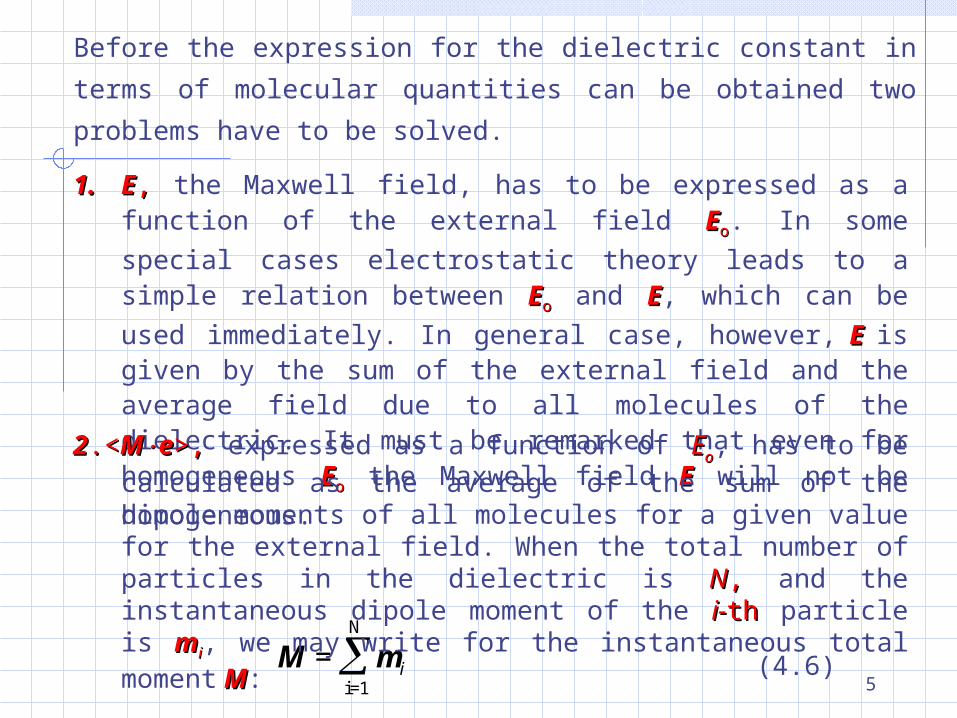
Before the expression for the dielectric constant in terms of

molecular quantities can be obtained two problems have to be

solved.

1.1. EE,, the Maxwell field, has to be expressed as a function of the external field EEoo. In some special cases electrostatic

theory leads to a simple relation between EEoo and EE, which

can be used immediately. In general case, however, EE is given by the sum of the external field and the average field due to all molecules of the dielectric. It must be remarked that even for homogeneous EEoo the Maxwell field

EE will not be homogeneous.

M m=i=

N

i1 (4.6)

22.<.<MMee>,>, expressed as a function of EEoo, has to be calculated as the average of the sum of the dipole moments of all molecules for a given value for the external field. When the total number of particles in the dielectric is NN,, and the instantaneous dipole moment of the i-i-thth particle is mmii, we may write for the instantaneous total moment MM:

6

Let us take a region with NN molecules which are treated explicitly; the remaining NN--NN molecules are considered to form a continuum and are treated as such. The approximations in this method can be made as small as necessary by taking NN sufficiently large. If this value of NN is still manageable in the calculations, the method can be used to introduce the molecular interactions into the calculation of the dielectric constant of polar liquids.

Non-polarizable molecules (rigid Non-polarizable molecules (rigid dipoles)dipoles) Non-polarizable molecules (rigid Non-polarizable molecules (rigid dipoles)dipoles) Let us consider the idealized case that the polarizability of the molecules can be neglected, so that only the permanent dipole moments have to be taken into account. We are taking a sphere of volume VV, containing NN molecules. For convenience in the calculations we suppose that it is it is embedded in its own materialembedded in its own material, which extends to infinity. The material outside the sphere can be treated as a continuum

with dielectric constant In this case the external field working in the sphere is the cavity field (eqn.2.14):

7

E = E E0 C

3

2 1

(4.7)

where EE is the Maxwell field in the material outside the sphere. We can substitute (4.6) in the general expression for the dielectric constant of homogeneous, isotropic dielectric:

1 41 1

30

00

20= N

E

E N kTNM

E

e A e(4.8)

where NN==NN /V/V is the number density, and the tensor Atensor A plays the role of a polarizability; 0

1,0

2

N

jijiM Because we defined that

themolecules are non polarizable, <<eeAAee>>oo=0.=0. In this case after substitution of (4.7) into (4.8), we obtain:

14 3

2 1 3

20=

V

M

kT(4.9)

The average of the square of the total moment can be calculated as follows in the case of non-polarizable molecules:

8

so that we may write:

In this equation the superscript NN to dXdX to emphasize that the integration is performed over the positions and orientations of NN molecules. The integration in the numerator of eqn.(4.11) can be carried out in two steps.

N

i

i

kTUdX

kTUdXM

10

2

)/exp(

)/exp(N

N M(4.11)

M =i=

N

i1 (4.10)

Since ii is a function of the orientation of the i-thi-th molecule

only, the integration over the positions and orientations of all other molecules, denoted as NN -i-i, can be carried out first. In this way we obtain (apart from a normalizing factor) the average moment of the sphere in the field of the i-thi-th dipole

with fixed orientation. The averaged moment, denoted by MMii*,*,

can be written as:

9

The average moment MMii** is a function of the position and orientation of the ii-th-th molecule only. Expression (4.12) for MMii** can be substituted into eqn. (4.11). Denoting the position and orientation coordinates of the i-th molecule by XXii and using a weight factor p(Xp(Xii))

)/exp(

)/exp(1

1

*

kTUdX

kTUdXi

N

N MM (4.12)

)/exp(

)/exp()

1

kTUdX

kTUdXp(X i

N

N

(4.13)

i*ii

i

i

i*ii

i dXXpdXXpM

MM ((1

0

2 NN

(4.14)

since after integration over the positions and orientations of molecule i,i, the resulting expression will not depend on the value of ii.

We obtain:

10

Before we substitute the expression for <M<M22>>oo into eqn.(4.9) , we note that it is possible to rewrite expression (4.14) in suggestive form. According to eqn.(4.12) and (4.13) MMii** can be written as the sum of moments jj,, averaged with the orientation of the ii-th-th dipole held fixed. denoting the angle between the orientation of the ii-th-th and the jj-th-th dipole by ijij,, this leads to:

N

N

N

j=1

ij

iikTUdX

kTUosdX

)/exp(

)/exp(1

1

*

c

M (4.15)

N

N

N

1

2

0

2

)/exp(

)/exp(cos)(

j

i

i

iji

i dXkTUdX

kTUdXXpNM

-

- (4.16)

and thus to:

This expression for <M<M22>>oo can be abbreviated by introducing

the average of coscosijij, defined as:

i

i

iji

iij dX

kTUdX

kTUdXXp

)/exp(

)/exp(cos)(cos

-

-

N

N (4.17)

11

We then write:

N

N1

20

2 cosj

ijM (4.18)

If we now substitute Eqn. (4.14) or its another form (4.18) into (4.9) we find after some rearrangements, and using NN==NN/V/V for the number density:

( -1)(2 + 1)

12

N

kTp X dX

N

kTii

ijj3 3

2

1

( cosii* M

N

(4.19)

Let us compare this expression with (3.34) from the previous lecture, for a special case of a pure dipole liquid with non-non-polarizable moleculespolarizable molecules (=0):

( -1)(2 +1)

12

N

kT32 (4.20)

This expression was derived in previous lecture with the help of the continuum approach, in which a sphere containing sphere containing only one moleculeonly one molecule is used. Therefore the (4.20) is a special case of (4.19) when the sphere containing NN molecules is restricted to one, MMii** = =ii and coscosijij is equal to 11.

12

When the sphere contains more than one molecule, the value of MMii** can be different from ii . When the number of molecules

included in the sphere increases, MMii** reaches a limiting value,

so that MMii** will be independent of NN as long as N N exceeds a

certain minimum value. The dipole moment MM of a sphere in the field of an arbitrary charge distribution within it, is given by:

M m

1

2(4.21)

where mm is the dipole moment of the charge distribution. Since this expression for M M does not depend on the radius of the sphere, the dipole moment of a spherical shell in the field of a point dipole within the inner sphere must be zero.

This conclusion will also hold if the sphere is not in vacuum,

but embedded in a dielectric, even with same dielectric but embedded in a dielectric, even with same dielectric

constant as the sphere itselfconstant as the sphere itself.

13

From this argument we conclude that the deviations of Mthat the deviations of Mii* *

from the value from the value i i are the result of molecular interactions are the result of molecular interactions

between the i-th molecule and its neighborsbetween the i-th molecule and its neighbors..

Thus the addition of a number of molecules contained in a spherical shell to original number NN will not change the moment of the sphere as long as the spherical shell can be treated macroscopically.

It is well known that liquids are characterized by short-range order and long-range disorder. The correlations between the orientations (and also between positions) due to the short-

range ordering will lead to values of MMii** differing from ii. This

is the reason that Kirkwood Kirkwood introduced a correlation factor gg

which accounted for the deviations of

p X dXii

ijj

( cosii*

M 2

1

N

from the value 22:

14

g p X dXii

ijj

12

1( cosi

i* M

N

(4.22)

With the help of this definition, eqn. (4.19) may be written as:

( -1)(2 + 1)

12

N

kTg

32

(4.23)

When there is no more correlation between the molecular orientations than can be accounted for with the help of the continuum method, one has g=1g=1 we are going to OnsagerOnsager relation for the non-polarizable case, for rigid dipoles with

=1=1. An approximate expression for the Kirkwood correlation factorKirkwood correlation factor can be derived by taking only nearest-neighbors interactions into account. In that case the sphere is shrunk to contain only the i-thi-th molecule and its zz nearest neighbors. We then have:

15

Mi

i j

z

dX U kT

dX U kT*

exp( / )

exp( / )

N

N

1

1

j=1 (4.24)

with N=z+1.N=z+1. Substitution this into (4.22) and using the fact that the material is isotropic, we obtain:

g p X dXdX U kT

dX U kTi i

iij

ij

z

1 + ( )cos exp( / )

exp( / )

N -

N -

1(4.25)

Since after averaging the result of the integration will be not

depend on the value of jj,, all terms in the summation are equal

and we may write: ijcosz1g ijcosz1g (4.26)

Since coscosijij depends only on the orientation of the two

molecules, all other coordinates can be integrated out and we

may write:

16

)kT/Uexp(dd

)kT/Uexp(cosddcos

ji

ji

ji

ijji

ij (4.27)

where ii and jj denote the orientation coordinatesorientation coordinates of the i-thi-th

and the j-thj-th molecules, and is a rotational intermolecular interaction energy, averaged over all positions and the orientations of all other molecules.

jiU

When the molecules prefer an ordering withWhen the molecules prefer an ordering with anti-parallel anti-parallel dipoles, dipoles, gg <1 <1.When the molecules prefer an ordering withWhen the molecules prefer an ordering with anti-parallel anti-parallel dipoles, dipoles, gg <1 <1.

It is clear from eqn. (4.27) that

 gg will be different fromwill be different from 11 when when <cos<cosijij>>0,0, i.e. when there i.e. when there

is correlation between the orientations of neighboring is correlation between the orientations of neighboring molecules. molecules.

 gg will be different fromwill be different from 11 when when <cos<cosijij>>0,0, i.e. when there i.e. when there

is correlation between the orientations of neighboring is correlation between the orientations of neighboring molecules. molecules. When the molecules tend to direct themselves withWhen the molecules tend to direct themselves with parallel parallel dipole momentsdipole moments, , <cos<cosijij> will be positive and > will be positive and gg>1>1..When the molecules tend to direct themselves withWhen the molecules tend to direct themselves with parallel parallel dipole momentsdipole moments, , <cos<cosijij> will be positive and > will be positive and gg>1>1..

17

Polarizable Polarizable MoleculesMoleculesPolarizable Polarizable MoleculesMoleculesLet as consider the system of NN identical molecules with permanent dipole strength and scalar polarizabilities . The

i-thi-th molecule is located at a point with radius vector rri i and has

an instantaneous dipole moment mi. This dipole moment will

be given by:

where ((EE11))ii, the local field at the position of the i-thi-th molecule

for a specified configuration of the other molecules, is given by:

iii )( 1Eμm (4.28)

j

N

ijiji mTEE

01

(4.29)

In this equation EEoo is the external field and -TTij ij · · mmjj is the field

at rri i due to a dipole moment mmjj at rrii. We can also define the

3333-dimensional dipole-dipole interaction tensor TTijij,

connected with the molecules i and jj..

18

In the case of polarizable molecules the total moment of the

sphere in KirkwoodKirkwood approximation will be given by:

M p=i=

i i1

N

(4.30)

where ppii is the induced moment of the i-thi-th molecule. The

induced moment ppii is a function of the positions and

orientations of all other molecules. Taking into account (4.28)

we can write:

ii ii )( - 1Eμmp (4.31)

The local field depends on the positions and orientations of all

other molecules. Therefore it is not possible to perform the

integrations in <<MM22>>oo in two steps , as we did in the non-

polarizable case.

19

Approximation of FröhlichApproximation of Fröhlich Approximation of FröhlichApproximation of Fröhlich

For the representation of a dielectric with dielectric permittivity , consisting of polarizable molecules with a permanent dipole moment, FröhlichFröhlich introduced a continuum continuum

with dielectric constant with dielectric constant in which point dipoles with a

moment dd are embedded. In this model each molecule is

replaced by a point dipole dd having the same non-

electrostatic interactions with the other point dipoles as the molecules had, while the polarizabilitypolarizability of the molecules can be imagined to be smeared out to form a continuum with

dielectric constant .

Let us also split polarization PP in two parts:

the induced polarizationthe induced polarization P Pinin and the orientation polarizationthe orientation polarization PPororThe induced polarizationinduced polarization is equal to the polarization of the continuum with the , so that we can write

EPin

4

1 (4.32

)

20

The orientation polarization is given by the dipole density due

to the dipoles dd. If we consider a sphere with volume V V

containing N N dipoles (as we did in non-polarizable case), we can write:

eMP dor V

1(4.33)

where:

Md d i=

i=

1

N

(4.34)

<<MMdd··ee>,>, the average component in the direction of the field,

of the moment due to the dipoles in the sphere, is given by an expression :

)exp(

)exp(1

1

U/kTdX

U/kTedXe

d

d

N

N MM< (4.35

)

21

Here UU is the energy of the dipoles in the sphere. This energy consists of three parts:

The external field in this model is equal to the field within a spherical cavity filled with a continuum with dielectric constant , while the cavity is situated in a dielectric with dielectric constant (Fröhlich field Fröhlich field EEFF ).

The field of this cavity field with dielectric will be:

E EF

3

2

(4.36)

3.3. the non-electrostatic interaction energythe non-electrostatic interaction energy (London-Van der Waals energy) between the molecules which is responsible for the short-range correlation between orientations and positions of the molecule.

2.2. the electrostatic interaction energy of the dipolesthe electrostatic interaction energy of the dipoles

1.1. the energy of the dipoles in the external fieldthe energy of the dipoles in the external field

22

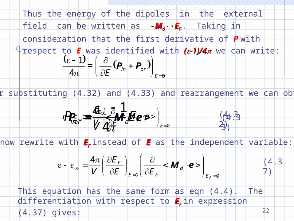
Thus the energy of the dipoles in the external field can be

written as --MMdd··EEFF. Taking in consideration that the first

derivative of P with respect to E was identified with ((-1)/4-1)/4 we can write:

04

1

EorinE

PP=

after substituting (4.32) and (4.33) and rearrangement we can obtain:

0

4

E

dEVeM

We now rewrite with EEFF instead of EE as the independent variable:

0

4

FE

dF0E

F

EE

E

VeM (4.37

)

This equation has the same form as eqn (4.4). The differentiation with respect to EEFF in expression (4.37) gives:

EPin

4

1 (4.32

) eMP dor V

1(4.33)

23

3kT

M

E

E

V0

2d

0E

F

4

(4.38)

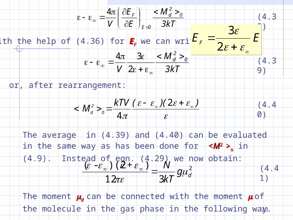
With the help of (4.36) for EEFF we can write :

3kT

M

V0

2d

2

34 (4.39)

or, after rearrangement:

Md

2

0

kTV

4

2

( )( ) (4.40

)

The average in (4.39) and (4.40) can be evaluated in the same way as has been done for <<MM2 2 >>oo in (4.9). Instead of

eqn. (4.29) we now obtain: 2

3

12

)+)(2-(dg

kT

N

(4.41

)

The moment dd can be connected with the moment of the

molecule in the gas phase in the following way.

E EF

3

2

E EF

3

2

24

In terms of the simplified model, evaporation consists in the disengagement of small spheres with dielectric constant

and a permanent dipole moment dd in the center. The moment

mm of such a sphere in vacuum consists of the permanent moment dd and the moment induced by dd in the surrounding dielectric:

ddd μμμm2

3

2

1

(4.42)

Obviously, mm must be set equal to the moment of the molecule in the gas phase. In this case we find:

μμ3

2

d

(4.43)

Substituting eqn.(4.43) into eqn.(4.41), we obtain after simple rearrangement:

Equation (4.44) is called the KirkwoodKirkwood-Fröhlich equation.

gkT

2

2

9

4

2

2

gkT

2

2

9

4

2

2

(4.44)

25

This equation gives the relation between , dielectric permittivity, , the dielectric permittivity of induced polarization, the temperaturetemperature, the densitydensity, and the permanent dipole momentpermanent dipole moment, for those cases where the intermolecular interactions are sufficiently well known to calculate Kirkwood correlation factor Kirkwood correlation factor gg. If there is no specific correlations one has g=1. If there is no specific correlations one has g=1.

If the correlations are not negligible, detailed If the correlations are not negligible, detailed information about the molecular interactions is information about the molecular interactions is required for the calculations of required for the calculations of gg..

If there is no specific correlations one has g=1. If there is no specific correlations one has g=1.

If the correlations are not negligible, detailed If the correlations are not negligible, detailed information about the molecular interactions is information about the molecular interactions is required for the calculations of required for the calculations of gg..

For associating compounds, where the occurrence of hydrogen bondshydrogen bonds makes relevant the assumption that only certain specific angles between the dipoles neighboring molecules are possible the molecular interactions may be represented by simplified models. Let us derived this extended equation for those compounds where the molecules or the polar segments form clusters of limited size. Consider each kind of polymers or multimers as a separate compound and neglecting any specific correlation between the total dipole moments of the polymers or multimers we can try the general equation for the polar fluids:

26

nn

nn

n nn

n

fkTf

N

f

N

13

1

1112

1)+1)(2-(

100

00

= (4.45)

where index oo refers to the non-polar solvent, and index nn refers to the polymers or multimers containing nn polar units. The average is taken over all conformations of the polymer or multimer. The upper limit of the summation can be extended to infinity since NNnn, the number of n-mersn-mers per cm3, becomes zero when nn becomes large. The polarizability oo can be calculated from the Clausius-MossottiClausius-Mossotti equation for the pure solvent.

2

n

ANd

M

0

0

0

00 2

1

4

3

(4.46)

Combining the Clausius-MossottiClausius-Mossotti equation and the Onsager Onsager approximation for the radius of the cavity, we have

1

1

2 1

2

2

30 0 0

0

f

(4.47)

27

We assume that the polarizabilities and the molecular volumes of the n-mersn-mers are proportional to nn, so that:

n n 1(4.48)

where 1

1

1

3

4

1

2

M

d N A

(4.49)

Here, dd is the density and is the dielectric constant of

induced polarization of the polar compound in the pure state. In the same way we find, using Onsager's approximation for the radius of the cavity:

We now substitute equations (4.46) - (4.50) into (4.45) and divide both members by (2(2+1),+1), obtaining:

3

2

2

12

1

1

nnf

(4.50)

1

2

2

2

11

1

00

000

227

212

24

1

24

1

12

1

nnn

nn

AA

N)(kT

))((

nNNd)(

M)(

Nd)(

M)(N

(4.51)

28

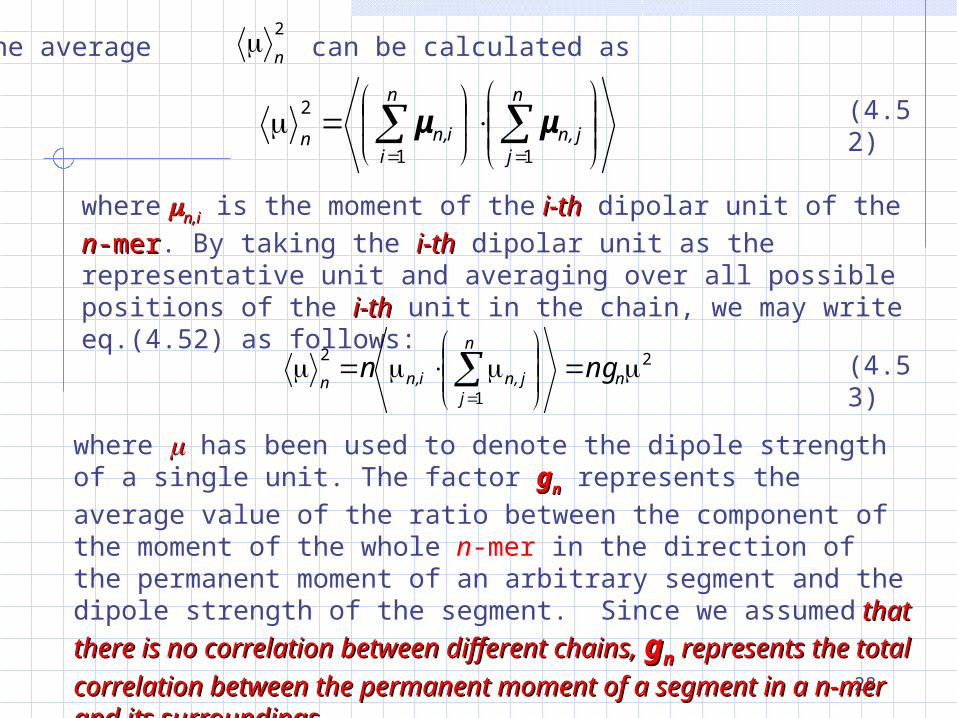
The average can be calculated as 2

n

n

jj,n

n

ii,nn

11

2μμ (4.52

)

where n,in,i is the moment of the i-thi-th dipolar unit of the nn-mer-mer. By taking the i-thi-th dipolar unit as the representative unit and averaging over all possible positions of the i-thi-th unit in the chain, we may write eq.(4.52) as follows:

2

1

2

n

n

jj,ni,nn

ngn (4.53)

where has been used to denote the dipole strength of a single unit. The factor ggnn represents the average value of the ratio between the component of the moment of the whole n-mer in the direction of the permanent moment of an arbitrary segment and the dipole strength of the segment. Since we assumed that there is no correlation between different chains, that there is no correlation between different chains,

ggnn represents the total correlation between the permanent represents the total correlation between the permanent

moment of a segment in a n-mer and its surroundings.moment of a segment in a n-mer and its surroundings.

29

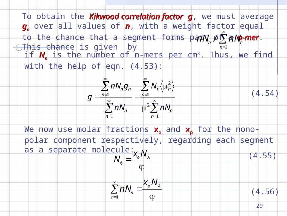
To obtain the Kikwood correlation factorKikwood correlation factor gg, we must average ggnn over all values of nn, with a weight factor equal to the chance that a segment forms part of a n-mern-mer. This chance is given bynN nNn n

n

/

1

if NNnn is the number of n-mers per cm3. Thus, we find with the help of eqn. (4.53):

1

2

1

2

1

1

nn

nnn

nn

nnn

nN

N

nN

gnNg (4.54)

We now use molar fractions xxoo and xxpp for the nono-polar component respectively, regarding each segment as a separate molecule:

Nx No A

0 (4.55)

nNx N

nn

p A

1 (4.56)

30

In these equations =(x=(xooMMoo+x+xppMM11)/d)/d denotes the molar volume of the mixture. Substituting eqns. (4.54)-(4.56) into eqn.(4.51) we find:

1

12

1

4 2

1

4 2

2 1 2

27 2

0 0 0

0 0

1

1

2

2

2

x M

d

x M

d

x N

kTg

p

p A

( )

( )

( )

( )

( )( )

( ) (4.57)

From this it follows:

gkT

N x

x M

d

x M

d

A p

p

22

2

0 0 0

0 0

1

1

9 2

4 2 1 2

1 3 1

2

3 1

2

( )

( )( )

( ) ( )

( )

( )

( ) (4.58)

This equation makes possible the calculation of the Kirkwood correlation factor correlation factor gg from experimental data for solutions of associating or polymeric compounds in non-polar solvents.