EE 370L

Controls Laboratory

Laboratory Exercise #9

PID Control

Department of Electrical and Computer Engineering

University of Nevada, at Las Vegas

1. Learning Objectives

To demonstrate the concept of proportional-integral-differential (PID) control.

2. Equipment Usage

In this laboratory exercise, you will be exposed to the PID controller. You will use

MATLAB and SIMULINK software to design a PID controlled feedback system.

3. Fundamentals

In applications where a simple gain compensator is inadequate to achieve stability or

other performance specifications, a frequency-dependent (dynamic) compensator is

needed. One of the earliest such compensators was the PID controller. The PID control

does not require a detailed model of the plant. Compensator is designed by “tuning” its

parameters while the system is operational.

A PID compensator has the transfer function of the following form:

s

K

Ks

K

KsK

s

sKKsKsK

s

KKsGc

)(

)( 3

2

3

12

32

3213

21

As an example, consider the following closed-loop configuration.

which has two zeros and a pole at the origin. One zero and one pole can be designed as

ideal integrator; the other zero can be designed as ideal derivative compensator.

System “tuning” starts with varying K1 while other two parameters are set as zero (K2

=K3=0) while the system is operating. K1 is varied until system has an acceptable step

response i.e. drive e(t) toward zero.

If a steady-state error exist (ess0 0), K2 is adjusted. The term K2/s integrates error e(t)

and applies the result to the plant, forcing e(t) → 0. K2 is varied until sufficiently small

ess0 is achieved.

Finally, K3 is varied to reduce rise time of the output signal. This reduction of rise time

occurs since K3 provides extra “kick” at the start, when e(t) changes the most.

As mentioned above, PID tuning process does not require a detailed model of the plant.

The characteristics of the plant are discovered real-time as the compensator parameters

are adjusted. While PID control seems simple, it will not work for every system.

Nevertheless, PID control has proven to be a convenient method of compensation in a

variety of applications and is commonly used to this day, especially for controlling

simple systems or where a lengthy modeling and design process is unacceptable. Setting

K3 or K2 to zero yields two special cases of PID called PI and PD. These structures may

be used in applications where either the rise time or steady-state error is acceptable

without placing a third term in the compensator.

In some applications, the derivative term in the PID structure causes undesirable

phenomena, such as high-frequency noise or oscillations. In such cases, the compensator

frequency response can be attenuated at high frequency by introducing additional pole to

reduce these stray effects.

Design Steps:

1) Evaluate performance of the uncompensated systems and determine how much

improvement in transient parameter is required.

2) Design PD controller to meet the transient response specifications.

3) Simulate the system to see if transient specification requirements are met.

4) Redesign if specifications are not met.

5) Design PI controller to yield the required steady state error specifications.

6) Determine the gains, K1, K2 and K3.

7) Simulate the system to see if all specification requirements are met.

8) Redesign if all the specification parameters are not met.

Design Example:

Given the system shown in figure below:

Design the PID controller that meets the following specifications:

1) maintain 20% overshoot

2) reduce peak time to 2/3 of the uncompensated system’s peak time;

3) eliminate steady-state error

Step1: Uncompensated system performance:

1) 20% overshoot ↔ζ=0.456 line crosses the root locus at proportional gain K=121

achieves overshoot target;

2) Tp=0.297sec, must be reduced to ~0.2sec

3) e(∞)=0.156, must be reduced to 0

Step 2: Since we want to make the system response faster, we proceed with design of PD

controller. Peak required time is 2/3 of the uncompensated time. Therefore, imaginary

part of the dominant pole is

87.152.0

d

d

dT

and the real part of the dominant pole is

13.8117tantan 0

ddd

s

We find the necessary location of the compensator zero by requiring angular contribution

to the dominant pole at −8.13±j15.87 to be 180 degree. From root locus, sum of the

uncompensated system’s poles and zeros angular contribution at the desired dominant

pole is -198.37 degree. Therefore, contribution from the compensatory zero is 18.37

degree.

From the figure above,

92.5537.18tan13.8

87.15

c

c

zz

Thus PD controller is

Gpd = (s+55.92)

Root locus of the PD compensator is shown below:

From the root locus, PD gain is 5.34 at the desired point.

Steps 3 & 4: We simulate PD compensated systems to see if the transient specifications

are met. From simulation, we find reduction in rise time and improvement in steady state.

Step 5: Design ideal integrator to reduce steady state error. Any integral compensator

zero will work as long as the zero is placed closed to unity. Choosing ideal integrator:

s

ssGpi

5.0)(

We sketch root locus of the PID controlled systems as shown below:

From the figure above, we the dominant poles at −7.516±j14.67 with associated gain of

4.6 for damping ratio of 0.456.

Step 6: Now we determine K1, K2 and K3

s

ss

s

ssK

)96.2742.56(6.45.0)92.55(

2

Matching to the form s

sKKsK 2

321

K1 = 259.5

K2 = 128.6

K3 = 4.6

Steps 7 & 8: We simulate PID compensated systems to see if the transient specifications

are met.

4. Matlab Commands

The transfer function of the PID controller looks like the following:

Kp = Proportional gain

KI = Integral gain

KD = Derivative gain

The characteristics of P, I, and D controllers

CL RESPONSE RISE TIME OVERSHOOT SETTLING TIME S-S ERROR

Kp Decrease Increase Small Change Decrease

Ki Decrease Increase Increase Eliminate

Kd Small Change Decrease Decrease Small Change

Given the transfer function given below:

2010

1)(

2

sssH

The goal of this problem is to show you how each of Kp, Ki and Kd contribute to obtain

Fast rise time

Minimum overshoot

No steady-state error

Find Open Loop Response:

num=1;

den=[1 10 20];

step(num,den)

Running this m-file in the Matlab command window, you will get plot shown below.

The DC gain of the plant transfer function is 1/20, so 0.05 is the final value of the output

to a unit step input. This corresponds to the steady-state error of 0.95, quite large indeed.

Furthermore, the rise time is about one second, and the settling time is about 1.5 seconds.

Let's design a controller that will reduce the rise time, reduce the settling time, and

eliminates the steady-state error.

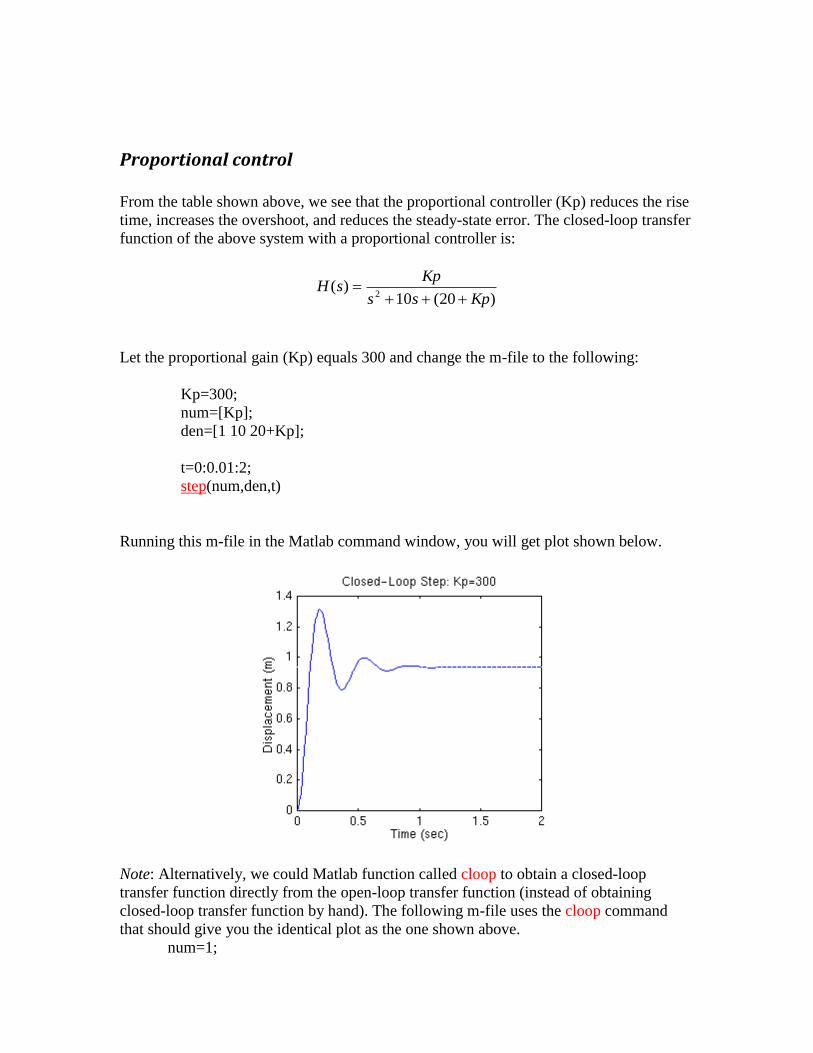
Proportional control

From the table shown above, we see that the proportional controller (Kp) reduces the rise

time, increases the overshoot, and reduces the steady-state error. The closed-loop transfer

function of the above system with a proportional controller is:

)20(10)(

2 Kpss

KpsH

Let the proportional gain (Kp) equals 300 and change the m-file to the following:

Kp=300;

num=[Kp];

den=[1 10 20+Kp];

t=0:0.01:2;

step(num,den,t)

Running this m-file in the Matlab command window, you will get plot shown below.

Note: Alternatively, we could Matlab function called cloop to obtain a closed-loop

transfer function directly from the open-loop transfer function (instead of obtaining

closed-loop transfer function by hand). The following m-file uses the cloop command

that should give you the identical plot as the one shown above.

num=1;

den=[1 10 20];

Kp=300;

[numCL,denCL]=cloop(Kp*num,den);

t=0:0.01:2;

step(numCL, denCL,t)

The above plot shows that the proportional controller reduced both the rise time and the

steady-state error, increased the overshoot, and decreased the settling time by a small

amount.

Proportional-Derivative (PD) control

From the table shown above, we see that the derivative controller (Kd) reduces both the

overshoot and the settling time. The closed-loop transfer function of the given system

with a PD controller is:

)20()10()(

2 KpsKds

KpKdSsH

Let Kp equals to 300 as before and let Kd equals 10, change the m-file to the following:

Kp=300;

Kd=10;

num=[Kd Kp];

den=[1 10+Kd 20+Kp];

t=0:0.01:2;

step(num,den,t)

Running this m-file in the Matlab command window, you will get plot shown below.

This plot shows that the derivative controller reduced both the overshoot and the settling

time, and had small effect on the rise time and the steady-state error.

Proportional-Integral control

From the table, we see that an integral controller (Ki) decreases the rise time, increases

both the overshoot and the settling time, and eliminates the steady-state error. For the

given system, the closed-loop transfer function with a PI control is:

KisKpss

KiKpSsH

)20(10)(

23

Let's reduce the Kp to 30, and let Ki equals to 70. Create a new m-file and enter the

following commands.

Kp=30;

Ki=70;

num=[Kp Ki];

den=[1 10 20+Kp Ki];

t=0:0.01:2;

step(num,den,t)

Running this m-file in the Matlab command window, you will get plot shown below.

We have reduced the proportional gain (Kp) because the integral controller also reduces

the rise time and increases the overshoot as the proportional controller does (double

effect). The above response shows that the integral controller eliminated the steady-state

error.

Proportional-Integral-Derivative control

Now, let's take a look at a PID controller. The closed-loop transfer function of the given

system with a PID controller is:

KisKpsKds

KiKpSKdssH

)20()10()(

23

2

After several trial and error runs, the gains Kp=350, Ki=300, and Kd=50 provided the

desired response. To confirm, enter the following commands to an m-file.

Kp=350;

Ki=300;

Kd=50;

num=[Kd Kp Ki];

den=[1 10+Kd 20+Kp Ki];

t=0:0.01:2;

step(num,den,t)

Running this m-file in the Matlab command window, you will get plot shown below.

Now, we have obtained the system with no overshoot, fast rise time, and no steady-state

error.

General tips for designing a PID controller When you are designing a PID controller for a given system, follow the

steps shown below to obtain a desired response.

1. Obtain an open-loop response and determine what needs to be improved

2. Add a proportional control to improve the rise time

3. Add a derivative control to improve the overshoot

4. Add an integral control to eliminate the steady-state error

5. Adjust each of Kp, Ki, and Kd until you obtain a desired overall response. You

can always refer to the table shown in this "PID Tutorial" page to find out which

controller controls what characteristics.

Lastly, please keep in mind that you do not need to implement all three

controllers (proportional, derivative, and integral) into a single

system, if not necessary. For example, if a PI controller gives a good

enough response (like the above example), then you don't need to

implement derivative controller to the system. Keep the controller as

simple as possible.

5. Prelab

1) Construct a Simulink model of the PID controller.

2) Plot the PID controller response for the following uncompensated transfer

function:

2012

1)(

2

sssH

6. Submission

For the simple feedback system shown below, perform the following tasks.

.

)20(

1)(

sssG

TASK: Use the Simulink model constructed in prelab to find Kp, Kd and Ki of the PID

controller that meets the following specifications:

Percent overshoot: < 5%

Settling time: < 250 ms

Maximum response to a unit disturbance: < 5X10-3