1

Joint multi-mode dispersion extraction in Fourierand space time domains

Sandip Bose, Member, IEEE, Shuchin Aeron, Member, IEEE, and Henri-Pierre Valero

Abstract

In this paper we present a novel broadband approach for the extraction of dispersion curves of multiple timefrequency overlapped dispersive modes such as in borehole acoustic data. The new approach works jointly inthe Fourier and space time domains and, in contrast to existing space time approaches that mainly work for timefrequency separated signals, efficiently handles multiple signals with significant time frequency overlap. The proposedmethod begins by exploiting the slowness (phase and group) and time location estimates based on frequency-wavenumber (f-k) domain sparsity penalized broadband dispersion extraction method as presented in [1]. In thiscontext we first present a Cramer Rao Bound (CRB) analysis for slowness estimation in the (f-k) domain andshow that for the f-k domain broadband processing, group slowness estimates have more variance than the phaseslowness estimates and time location estimates. In order to improve the group slowness estimates we exploit thetime compactness property of the modes to effectively represent the data as a linear superposition of time compactspace time propagators parameterized by the phase and group slowness. A linear least squares estimation algorithmin the space time domain is then used to obtain improved group slowness estimates. The performance of the methodis demonstrated on real borehole acoustic data sets.

Index Terms

Dispersion extraction, sparsity, continuous wavelet transform, space time methods

I. INTRODUCTION

Acoustic data collected by borehole logging tools is dominated by wave guided propagating modes. Such modesare usually dispersive, that is, each mode propagates at a slowness (inverse of velocity) that varies as a function offrequency. This dispersion or frequency dependent variation of phase slowness is an important characteristic of suchmodes and is now understood as conveying useful information about the rock formations traversing the borehole[2], [3], [4]. Existing techniques for dispersion extraction employ a frequency by frequency processing or so callednarrowband processing and extract the wavenumber at each frequency using uniform linear array (ULA) processingtechniques such as the Prony [5] and matrix pencil [6] methods for analyzing exponentials. A number of otherapproaches for dispersion analysis have been proposed such as phase minimization or coherency maximization[7], or slowness frequency coherence based methods [8], [9]. Although adequate for analyzing strong signals inlow to moderate noise situations, i.e with favorable signal to noise ratio (SNR), these narrowband approaches failto identify all the modes of interest, especially the weaker ones, and may not be robust and accurate enough forquantitative interpretation even for such strong signals due to scatter and aliasing in the results. This is particularlyan issue in logging while drilling (LWD) scenarios where the SNR could be low and there could be significantinterference and model deviation due to the drilling process and the presence of a heavy drill collar moving w.r.t. theborehole. Wireline logging scenarios involving more complex physics such as in cased hole or deviated wells mayalso prove challenging for such methods. Other array processing methods such as ESPRIT and MUSIC, [10], [11]can be employed here but are sensitive to the choice of model order , [11, Chapter 16], and the knowledge of signalsubspace. Schemes such as in [12], [11] based on minimum description length (MDL), [13] have been proposedto estimate the signal subspace and the model order. However these methods work fine under some stationarityassumptions on the signal and are not applicable to borehole acoustic logging where the signal is transient and

Sandip Bose is with the Math and Modeling Department, Schlumberger Doll Research (SDR), Cambridge, MA, USA. e-mail:bose1@slb.com

Shuchin Aeron is with the Dept. of Electrical and Computer Engineering (ECE) at Tufts University, Medford, MA, USA. e-mail:shuchin@ece.tufts.edu

Henri-Pierre Valero is with SKK, Japan. e-mail:hvalero@slb.com

arX

iv:1

312.

3981

v1 [

phys

ics.

geo-

ph]

13

Dec

201

3

2

highly non-stationary. Thus narrowband methods are inherently limited for the quantitative extraction of modaldispersion curves.

Therefore there is a need for an efficient broadband dispersion extraction algorithm that does not requireassumptions of stationarity, and is robust to noise and presence of strong interference due to the coherent processingof the signal over a frequency band. A broadband approach for extraction of a single mode dispersion was proposedin [14] which is limited to a particular type of borehole mode namely the lowest order flexural mode of an openborehole or one where the effect of the tool is well characterized. A more general approach for extracting dispersionof a single mode without reference to a physical model or restriction of the type of mode was proposed in [15] and[16]. There the continuous wavelet transform (CWT) of the array data was employed along with a parameterizationof the wavenumber dispersion in the f − k domain in terms of a local first order linear approximation at eachfrequency. It was shown that under such an approximation around the center frequency at any given scale, the shiftsin the CWT coefficients at that scale across the receivers is proportional to the group slowness and the phase changeis dependent on both phase and group slowness. This property was exploited in [16] to estimate the dispersionparameters in the CWT domain using a modification of the Radon transform called the exponentially projectedRadon transform (EPRT). Although broadband in nature, with good performance for multiple modes in situationswhere there is significant time separation, these methods have poor performance for multiple modes with significanttime overlap in the modes. Similar ideas that exploit the time frequency localization have been considered before,e.g., the energy reassignment method of [17] which has been applied in [18] for analysis of dispersion of Lambwaves. Again these methods are suitable when the time-frequency separation of modes is good but fails otherwise.In [19] a broadband method based on linear approximation of the dispersion curves in the (f − k) domain wasproposed. However this method is still based on some stationarity assumptions on the signal which, as pointed outbefore, does not hold true for real signals obtained with pulsed excitation in downhole logging tools.

In this context in [1] the authors proposed a novel sparsity penalized broadband dispersion extraction method inthe f−k domain which has been shown to be robust to the presence of time overlapped modes. The key ingredientthere was to first propose an overcomplete dictionary of broadband propagators for representation of array datafollowed by exploiting the sparsity in the number of modes, manifested as simultaneous sparsity, see [20], in therepresentation coefficients at each frequency scale. In this framework as shown in [1], a sparsity penalized recoveryalgorithm leads to dramatic improvements in performance under heavy noise conditions. However the approachis not at par with semblance based processing techniques such as the space time coherence (STC) processing ofnon-dispersive waves, [21], or of dispersive modes such as EPRT, [16], which are more reliable for direct estimationof group slowness. The main reason is that unlike STC based techniques such as EPRT, we don’t exploit the localspatio-temporal coherence of modes in space-time domain. This leads to increased variance in the group slownessestimates from f − k domain processing as shown by a Cramer-Rao Bound (CRB) analysis in the Appendix ofthis paper. To overcome this drawback, in this paper we combine the two techniques of [1] and [16] and proposea joint f − k and space-time domain multimode dispersion extraction method.

The organization of the paper is as follows. The next section II introduces the problem setup and formulationof the approach using the CWT and reviews the use of the broadband f − k processing for the dispersionestimation. Section III presents the proposed space-time approach to refine the dispersion estimates. Section IVcovers application of the new approach to a diverse series of real data examples indicating the improvement in thequality of the estimates. Finally some performance analysis on is included in the appendix VI after the conclusion.

II. PROBLEM SET-UP AND BROADBAND FORMULATION

A. Preliminaries

Acoustic waves are excited in the borehole by firing a source which produces modes with the borehole as awaveguide. A schematic is shown in Figure 1. The relation between the received waveforms and the frequency-wavenumber (f − k) response of the borehole to the source excitation is captured via the following equation,

sl(t) =

∫ ∞0

∫ ∞0

S(f)Q(k, f)ei2πfte−i2πkzldfdk (1)

for l = 1, 2, ..., L, where sl(t) denotes the pressure at time t at the l-th receiver located at a distance zl from thesource; S(f) is the source spectrum and Q(k, f) is the wavenumber-frequency response of the borehole. Typically

3

the data is acquired in presence of noise (environmental and receiver noise) and interference which we collectivelydenote by wl(t). Then the noisy observations at the set of receivers, yl(t), l = 1, . . . , L, can be written as,

yl(t) = sl(t) + wl(t) (2)

It has been shown that the complex integral in the wavenumber (k) domain in Equation(1) can be approximatedby the contribution due to the residues of the poles of the system response, [2], [22]. Specifically,∫ ∞

0Q(k, f)e−ikzldk ∼

M(f)∑m=1

qm(f)e−(i2πkm(f)+am(f))zl (3)

where qm(f) is the residue of the m-th pole and respectively where km(f) and am(f) are the corresponding realand imaginary parts of the poles and can be interpreted as the wavenumber and attenuation respectively as functionsof frequency. This means that we have

sl(t) =

∫ ∞0

M(f)∑m=1

Sm(f)e−(i2πkm(f)+am(f))zlei2πftdf (4)

where Sm(f) = S(f)qm(f). In theory the number of modes can be infinite but in practice only a few are significant,i.e. the model order M(f) is finite and is small. In the scope of this work, we will assume that M(f) = M for allthe frequencies of interest. Under this signal model, the data acquired at each frequency across the receivers canbe written as,

Y1(f)Y2(f)

...

...YL(f)

︸ ︷︷ ︸

Y(f)

=

e−(i2πk1(f)+a1(f))z1 . . . e−(i2πkM (f)+aM (f))z1

e−(i2πk1(f)+a1(f))z2 . . . e−(i2πkM (f)+aM (f))z2

... . . ....

e−(i2πk1(f)+a1(f))zL . . . e−(i2πkM (f)+aM (f))zL

S1(f)S2(f)

...

...SM (f)

︸ ︷︷ ︸

S(f)

+

W1(f)W2(f)

...

...WL(f)

︸ ︷︷ ︸

W(f)

(5)

In other words the data at each frequency is modelled as a superposition of M exponentials sampled with respect tothe receiver locations z1, .., zL. We refer to the above system of equations as corresponding to a sum of exponentialsmodel at each frequency.

We note that the modal dispersion is completely characterized in the (f−k) domain in terms of the wavenumberresponse k(f) as a function of frequency. This is often expressed in terms of related physical quantities - theslowness of the phase wavefront or the phase slowness, sφ(f), and the group slowness, sg(f) , which is thereciprocal of the energy transport velocity, both considered as functions of frerquency. These are related to thewavenumber and each other as follows:

sφ(f) =k(f)

f, sg(f) =

dk

df, sg(f) = sφ(f) + f

dsφ

df(6)

The dispersion extraction problem therefore consists in recovering the frequency dependent phase and groupslownesses of the mth mode, {sφm(f), sgm(f)} from the received data for m = 1, . . . ,M significant propagatingmodes. This is illustrated in Figure 1 where we observe two-three significant modes with a typical array acquisitionwith a borehole sonic tool such as described in [23]. Since we are going to use continuous wavelet transform (CWT)for dispersion extraction, in the next section we will provide a brief overview of the broadband dispersion extractionframework in the CWT domain and point out the time-frequency and space time properties of the acoustic modes.

Remark 2.1: In the following we will assume that the data is sampled temporally at at-least the Nyquist rateand that the total number of time samples is (say) T . Therefore we have a discrete time data Y ∈ RL×T fromwhich we want to extract the dispersion characteristics at the discrete set of DFT frequencies corresponding to thesampled system.

4

Phase Slowness

Group Slowness

Fig. 1. Schematic depicting the dispersion extraction problem for the case of borehole acoustic data. The figure illustrates an acoustic toolin the borehole generating energy that propagates as a sum of borehole guided modes each governed by a dispersion curve. The task is toestimate these dispersion curves given the waveforms received by an array of receivers on the tool as shown.

Fig. 2. Schematic showing the first order Taylor series approximation to the dispersion curve in a band around the center frequency fa ofthe mother wavelet at scale a.

B. Broadband dispersion extraction set-up in the CWT domain

Recall that the continuous wavelet transform (CWT) of a signal is obtained from the scalar product of this signalwith elements of a wavelet family generated by translations and dilations of a mother wavelet, g by T bDa[g(t)] =

1√ag( t−ba ). The CWT coefficients Cs(a, b) of the signal s(t) at the scale (dilation factor) a and shift (translation)

b is then given by

Cs(a, b) =1√a

∫s(t)g∗(

t− ba

)dt (7)

=

∫ ∞−∞

G∗(af)ei2πbfS(f)df (8)

where G(f) is the Fourier transform of the analyzing (mother) wavelet g(t) and S(f) is the Fourier transform ofthe signal being analyzed. The analyzing wavelet g(t) is chosen to satisfy some admissibility condition, see [24],[25] for details. The CWT generates a time-scale representation of a signal which indicates the frequency contentof the signal as a function of time. Such a representation is useful for dispersion analysis as explained below.

5

Consider the case of a mode m with spectrum Sm(f). Then under the exponential model, the CWT at scale aand time shift b of the received waveform at the l-th receiver is given by

Cml (a, b) =

∫ ∞−∞

G∗(af)Sm(f)ei2π(bf−zlkm(f))df (9)

. Equivalently by taking the Fourier transform with respect to b, one can write,

Cml (a, f) = G∗(af)Sm(f)e−i2πzlkm(f))df (10)

. Assuming that a first order Taylor series approximation holds true for the wavenumber in the effective frequencyband, Fa, around the center frequency fa of the analyzing wavelet, i.e. under the approximation (see Figure 2),

km(f) ≈ km(fa) + k′

m(fa)(f − fa), f ∈ Fa (11)

Cml (a, f) ≈ G∗(af)Sm(f)e−i2π(km(fa)+k′m(fa)(f−fa))zl , f ∈ Fa (12)

the CWT coefficients at scale a for the mth mode waveform at the l-th receiver can be expressed in terms of acorresponding quantity at a reference (0th) receiver,

Cml (a, b) = e−i2πδl(km(fa)−fak′m(fa))Cm0 (a, b− δlk

′

m(fa))

= e−iδlφm(fa)Cm0 (a, b− δlk′

m(fa)) (13)

where δl = zl − z0 denotes the spacing of the receiver l from the reference 0 and where φm(fa).= 2π(k(fa) −

fak′(fa)) = 2πfa(s

φ(fa)−sg(fa)) is a phase factor. Thus for a given mode the CWT coefficients of the mode at agiven scale undergo a time shift according to the group slowness across the receivers along with a complex phaseshift proportional to the difference of the phase and the group slowness. These ideas are depicted in Figure 3(a) &3(b). It becomes readily apparent that if the CWT coefficients corresponding to such a mode could be isolated andtime shifted by a given moveout, then the phase slowness sφm(fa) can be extracted by solving for an exponentialmodel when the moveout equals the group slowness sgm(fa).

The linearity of the CWT guarantees that in the presence of multiple modes and noise, the CWT of the data atscale a is the superposition of the CWT of each mode, i.e.,

Cl(a, b) ≈M∑m=1

e−iδl,φm(fa)Cm0 (a, b− δlk′

m(fa)) + Cwl (a, b) (14)

Cl(a, f) ≈M∑m=1

G∗(af)Sm(f)e−i2π(k(fa)+k′(fa)(f−fa))zl +W (a, f), f ∈ Fa (15)

where M is the number of modes, Cwl (a, b) is the CWT of the noise, and W (a, f) is the corresponding Fouriertransform. We observe that in the general case with time overlapped modes, we can no longer approach the problemin terms of shifting the CWT coefficients and solving a sum of exponentials model. However we can still representthe CWT coefficients in terms of broadband propagators using the above equation as detailed in the next section.First we make the following observations regarding the CWT coefficients of time compact propagating modes astypically seen in borehole acoustic logging:

1. Time compactness of mode m implies time compactness of the CWT coefficients Cml (a, b) at each scale. Thetime-frequency support of the modes in the CWT domain depends on the time-frequency uncertainty relationcorresponding to the mother wavelet used - at higher frequencies (smaller scales) the time resolution is sharpbut the frequency resolution is poor and vice-versa.

2. Time compactness in turn implies a linear phase relationship across frequencies f ∈ Fa in the Fourier transformcoefficients Cml (a, f) of the CWT data Cml (a, b) at any receiver l. This is depicted in Figure 4 for a syntheticexample.

It is worthwhile to note at this point that the first observation together with the dispersion relation of Equation 13in the CWT coefficients, formed the basis of EPRT processing as proposed in [16], appropriate when there is asingle dominant mode in the data or when the modes are well separated in time-frequency.

6

(a) (b)

Fig. 3. Combining the space-time and frequency-wavenumber processing for dispersion extraction using the CWT. Figure depicts the (a)(f −k) domain and (b) time domain characteristics of the CWT coefficients in terms of the propagation parameters at a given scale. The lefthand plot shows the linearized wavenumber dispersion curves of two overlapping modes in a frequency band corresponding to the frequencysupport of the CWT coefficients at scale a. The spectra of the CWT coefficients for each mode are also shown illustrating the support in theband around the center frequency fa. The right hand plot shows the real part of the corresponding CWT complex coefficients indicating theenvelope moveout given by the group slowness (frequency derivative of wavenumber) at fa and an inter-receiver phase shift given by thedifference between the phase and group slowness at fa. Both representations are used for robustly extracting the phase and group slownessestimates at various fa.

Fig. 4. An example of the implication of time compactness of the CWT coefficients at a given scale at one receiver on the phase of theFFT coefficients in the band. The lower panel depicts the real part of a typical CWT coefficient of a time compact synthetic signal at acertain scale a and plotted as a function of the shift parameter treated as a time index. The upper panel shows the unwrapped phase of theFFT of the CWT coefficient taken with respect to the time index and plotted as a function of frequency. This latter function manifests as astraight line with the slope related to the time location of the envelope peak of the CWT coefficients in the lower panel. The time locationestimate shown (190.89) is derived from the slope and is in good agreement with the true location of the envelope peak. This approach isused to estimate the time location of time-compact modes in the received data by application to the amplitude coefficients X−Fa obtainedby solving equation20.

7

C. Formulation in the CWT domain: sparse data representation using broadband propagators in f − k and z − tdomains

In this section we exploit the following aspects of mode characteristics, namely, (a) modes are nearly both time andfrequency compact at scale a and (b) the number of modes at scale a is small. Then working under the assumptionof the validity of the first order Taylor series approximation around the center frequency our methodology forbroadband dispersion extraction is centered around the following constructive representations of the CWT data atscale a in f − k and z − t domains respectively.

1) Broadband propagator representation in f −k domain over a frequency band Fa at scale a: In the followingwe will use a discrete set of frequencies f1, f2, ..., fNf ∈ Fa which correspond to the discrete DFT frequenciesunder the given sampling rate in the temporal domain. It is assumed that the temporal sampling is done at at-leastthe Nyquist rate.

Definition 2.1: A broadband propagator PF (k(fa), k′(fa)) (in band Fa) corresponding to a given phase

slowness k(fa)fa

and group slowness k′(fa) is a block diagonal matrix ∈ CL·Nf×Nf given by

PF (k(fa), k′(fa)) =

φ(f1)

φ(f2). . .

φ(fNf )

(16)

of sampled exponential vectors φ(f) given by

φ(f) =

e−i2π(k(fa)+k′(fa)(f−fa))(z1−z0)

e−i2π(k(fa)+k′(fa)(f−fa))(z2−z0)

...e−i2π(k(fa)+k′(fa)(f−fa))(zL−z0)

(17)

where z0 is a reference receiver.From Equation (15) one can easily see that the data in a given band is a superposition of M broadband propagators

PF (km(fa), k′

m(fa)). As proposed in [1] using this broadband representation in the f − k domain, a strategy toestimate the dispersion curves in the band Fa consists of the following.

1. At scale a form an over-complete dictionary of broadband propagators PF (k(fa), k′(fa)) in the (f−k) domain

spanning a range of group and phase slowness.2. Assuming that the broadband signal is in the span of the broadband propagators from the over-complete

dictionary, the presence of a few significant modes in the band implies that the signal representation in theover-complete basis is sparse. In other words that the signal is composed of a superposition of few broadbandpropagators in the over-complete dictionary.

3. The problem of slowness dispersion extraction in the band can then be mapped to that of finding the sparsestsignal representation in the over-complete dictionary of broadband propagators.

The over-complete dictionary is constructed using a range of phase slownesses sφi (fa) = ki(fa)fa

at the centerfrequency fa and a range of group slowness k

′

j , j = 1, 2, ..., n2 for the given band. The over-complete dictionaryof broadband propagators for acoustic signal representation in a band can then be written as

ΦaF =

[Φ1(Fa) | Φ2(Fa) | ... | ΦN (Fa)

]∈ CL.Nf×N.Nf (18)

where Φi+n1·(j−1)(Fa) = PF (ki(fa), k′

j(fa)) and N = n1 × n2 is the number of broadband basis elements in theover-complete dictionary.

It was shown in [1] that assuming that the constructed dictionary contains elements corresponding to the phaseand group slowness of the modes of interest, the CWT of the noisy data in band Fa denoted by

YFa = [Ya(f1)Ya(f2) . . .Ya(fNf )]T ∈ CL·Nf

at L receivers can be written as

YFa = ΦaFXFa(:) + WFa , XFa ∈ CNf×N (19)

8

for some unknown coefficient matrix XFa whose i + n1 · (j − 1)-th column corresponds to the CWT coefficientvector at the reference receiver z0, [C(i,j)(a, f1), C(i,j)(a, f2), ..., C(i,j)(a, fNf )]T corresponding to the mode withphase slowness sφi and group slowness sgj . Here (:) denotes the MATLAB (:) operator which vectorizes the matrixby stacking columns on top of each other. Since the number of modes M << N , XFa is column sparse, that is,only a few columns contain non-zero coefficient entries corresponding to the modes in the data. It was shown in[1] that in that case, one can recover the columnn-sparse coefficient matrix XFa and hence the modal dispersionby optimizing a sparsity penalized criterion,

OPT fk : XFa = arg min ||YFa −ΦFaXFa(:)||22 + λ∗||XFa ||1,2 (20)

where || · ||1,2 denotes the `1,2 norm, - computed by first forming the row-vector of `2 norms of the columns ofthe matrix followed by taking the `1 norm of the resulting row-vector - which has shown promise in recovery ofsparse structured matrices, [20]. The optimal λ∗ can be chosen using the strategy presented in [1] or can be set to√M logNσ2 if an estimate of the number of modes M and noise variance σ2 per-dimension is available.This approach to dispersion extraction was shown to be effective for recovering multiple modes overlapping in

time-frequency (or time-scale) domain and produced robust and accurate estimates of the phase slowness at thecenter frequencies fa for each scale used for analysis. However the group slowness estimates suffered from scatteras predicted by the Cramer Rao bounds for processing in the f − k domain wherein we do not exploit any timedomain compactness of the received signals. In order to do that we turn to broadband propagators in the space-timedomain which we now consider in this work.

D. Space-time (z − t) domain representation using time compact propagators with time-width Ta at scale a

We define a broadband propagator in space-time domain corresponding to a phase and group slowness as a timecompact window propagating at the group slowness with a complex phase change across receivers in proportion tothe difference of the phase and group slowness. Mathematically,

Definition 2.2: Let uTa(t) denote a rectangular window function of width Ta centered at zero. Then thebroadband space time propagator at a scale a is a real matrix of size T · L× T and given by,

Ua(sφ, sg, t0, Ta) =

ei2π(sφ−sg)fa(z1−z0)diag (uT (t− t0 + sg(z1 − z0)))

...ei2π(sφ−sg)fa(zL−z0)diag (uT (t− t0 + sg(zL − z0)))

(21)

where diag(·) is the MATLAB operator and z0 is a reference receiver.Examples of a broadband propagator in the space-time domain are shown in Figure 7. From Equation (14) it

can be seen that the data in the space time domain can be written as a superposition of M broadband propagatorsUa(sφm, s

gm, tm0 , Ta). Then similar to the f − k domain, using this broadband representation a similar strategy can

be employed in the space-time domain. Namely,1. At scale a form an over-complete dictionary of broadband propagators Ua(sφ, sg, t0, Ta) in the (z− t) domain

spanning a range of group and phase slowness and time locations.2. Assuming that the broadband signal is in the span of the broadband basis elements from the over-complete

dictionary, the presence of a few significant modes in the band implies that the signal representation in theover-complete dictionary is sparse. In other words that the signal is composed of a superposition of fewbroadband propagators in the over-complete dictionary.

3. The problem of slowness dispersion extraction in the band can then be mapped to that of finding the sparsestsignal representation in the over-complete dictionary of broadband propagators.

The overcomplete dictionary is constructed using a range of phase slownesses sφi (fa) = ki(fa)fa

at the centerfrequency fa, a range of group slowness k

′

j , j = 1, 2, ..., n2 and in addition a range of time points tr0, r = 1, 2, ..., n3

indicating the possible locations of the modes. The over-complete dictionary of broadband propagators for acousticsignal representation in a band can then be written as

Ua =[Ψ1(Ta) | Ψ2(Ta) | ... | ΨN ′(Ta)

]∈ RL·T×N ′·T (22)

where Ψi+n1·(j−1)+n1·n2·(r−1)(Ta) = Ua(sφi , s)jg, tr0, Ta) and N ′ = n1 · n2 · n3 is the number of broadband

propagators in the over-complete dictionary.

9

Let the CWT at scale a of the noisy data at L receivers be denoted by Ya ∈ CL×T . This data can be written as

Ya(:) = UaXTa(:) + W(:), XTa ∈ CT×N ′ (23)

for some unknown coefficient matrix XTa whose i+ n1 · (j − 1) + n1 · n2 · (r − 1)-th column corresponds to theCWT coefficient vector of length T at the reference receiver z0 and at time locations tr0,

[Ci,j,r(a, t1), Ci,j,r(a, t2), ..., Ci,j,r(a, tT )]T

corresponding to the mode with phase slowness sφi and group slowness sgj . Here (:) denotes the MATLAB (:)operator which vectorizes the matrix by stacking columns on top of each other. Since the number of modesM << N ′, similar to the f − k domain strategy one can solve for the estimation of modal dispersion and modespectrum (CWT) using the following optimization,

OPT zt : XTa = arg min ||Ya(:)− UaXTa(:)||22 + λ∗||XTa ||1,2 (24)

for some optimal value of λ∗.

III. JOINT f − k AND z − t PROCESSING OF CWT DATA AT SCALE a

Of the two approaches outlined above, clearly the approach using the broadband propagators in the z− t domainexploits all aspects of the modal properties, namely both time-frequency compactness and sparsity in the numberof modes. Nevertheless it is seen at once that due to the larger size of the optimization problem in the space timedomain solving for OPT zt is computationally very intensive and may not be feasible. Besides it requires one topick a good range for the arrival time of the modes to control the size of the dictionary. On the other hand OPT fkis quite tractable. Strictly speaking in the f − k domain, one can also incorporate time compactness of modesby imposing a linear phase constraint in the broadband (f − k) processing. However this would again imposesignificant additional computational requirements and is not feasible in general for practical applications. This isparticularly true when the computation has to be done at wellsite where computation speed and therefore efficiencyis critical.

Thus we propose a sequential method for dispersion extraction in the CWT domain that utilizes the broadbandmultiple mode extraction methodology in the (f −k) domain as proposed in [1] followed by the time compactnessof modes in the space-time domain in a manner similar to [16]. The main intuition is guided by a preliminaryCramer-Rao Bound (CRB) analysis carried out in Section VI, which shows that the broadband f − k processingresults in robust estimates of phase slowness and time locations of the mode while the group slowness estimates arenot as robust, see Figure 5 for an example on a synthetic data set. Here the variance in time location estimates ofeach mode are obtained using the CRB variance bounds on the corresponding coefficient phase estimates. We notethat it is possible to estimate the time locations by fitting a straight line to the coefficient phase across frequencyas discussed below; the computed variance in the latter then yield the corresponding quantity for the former.

Therefore in the sequential method below, we first estimate modal order, phase and group slownesses and thetime locations of the modes using the OPT fk. Then we update the group slowness estimates by a simple exhaustivesearch over a range of group slownesses around estimated ones for each mode using the broadband space-timepropagators. The proposed methodology consists of 3 steps at each scale -

A. STEP 1: Simultaneous sparsity penalized broadband dispersion extraction in f − k domain

Solve OPT fk and pick an initial set of modes by picking say R number of peaks from the vector colnorm(XFa) ∈R1×N and the corresponding phase and group slowness estimates along with the spectral estimates Crz0

(a, f)

corresponding to the r-th column of XFa . Proceed to the modal order selection and mode consolidation step below.Remark 3.1: The operation colnorm(·) for the matrix in the argument computes the `2 norms along the columns

and returns a row vector containing the norms. Mathematically for a matrix M ∈ Cm×n with entries Mij ,

colnorm(M) =

√√√√ m∑j=1

|M1j |2,

√√√√ m∑j=1

|M2j |2, ...,

√√√√ m∑j=1

|Mnj |2

The peak picking is done via an automatic procedure based on the relative amplitudes in vector colnorm(XFa).

10

Fig. 5. Figure showing the CRB for the slowness estimates for a two mode problem. One mode is 5-dB below the other mode. Note thatthe group slowness estimates are less robust than the phase slowness estimates and time location estimates (normalized by the transmitterreceiver spacing).

B. STEP 2: Model order selection and mode consolidation

In the broadband (f −k) processing proposed in [1] we performed the model order selection based on clusteringin the phase and group slowness domain. In contrast here we will perform the model order selection and modeconsolidation in the phase slowness and time location domain. In order to obtain the time location estimates weuse the fact that time compactness of the modes imply a linear phase relationship across frequency in the modespectrum. Based on the linear phase relationship one can obtain estimates of the time location of the modes at scale“a” from estimates of the mode spectrum at the reference receiver by fitting a straight line through the unwrappedphase of the estimated mode spectrum in the band. The slope of this line is related to the index of the time locationestimate of the mode via the relationship,

tr0 =slope(Unwrap. Phase Crz0

(a, f))2π.Ts.10−6

(25)

where Ts is the sampling time in µs. This is illustrated in figure 4.Example of mode clustering in the phase slowness and time location domain for a synthetic two mode case for

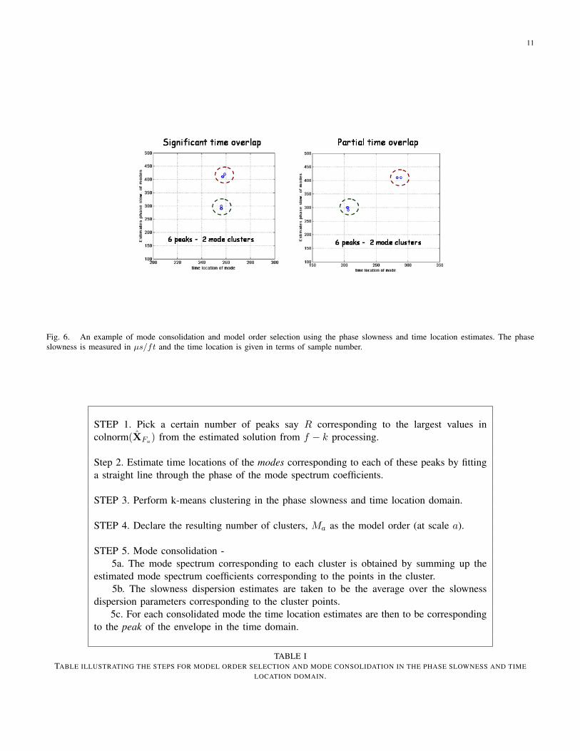
two scenarios of partial time overlap and total time overlap are shown in Figure 6. The R modes are clustered bya simple k−means clustering algorithm mode consolidation consists of averaging of the mode spectrum and thephase and group slowness estimates within each cluster. We denote the resulting model order by Ma. The timelocation estimates are not averaged but, for each consolidated mode the time location estimates are then estimatedfrom the location of the peak of the corresponding envelope in the time domain.

Steps 1. and 2. are summarized in Table I.

C. STEP 3: Space-time processing of the consolidated modes for refining mode spectrum and group slownessestimates

Let the declared number of modes from (f − k) processing at scale a be Ma. Let the corresponding phaseslowness estimates be given by sφm and let the time location estimates be given by tm0 for m = 1, 2, ...,Ma. Thetime window width T for each mode around the time location tm0 is based on the effective time width of theanalyzing wavelet at scale a. We pick a range of test moveouts for each mode around the estimated group slownessfrom the (f − k) processing. For an Ma-tuple of test moveouts say p = [p1, p2, ..., pMa

] we form space timepropagators using the phase slowness and time location estimates obtained from (f − k) processing. Then given

11

Fig. 6. An example of mode consolidation and model order selection using the phase slowness and time location estimates. The phaseslowness is measured in µs/ft and the time location is given in terms of sample number.

STEP 1. Pick a certain number of peaks say R corresponding to the largest values incolnorm(XFa) from the estimated solution from f − k processing.

Step 2. Estimate time locations of the modes corresponding to each of these peaks by fittinga straight line through the phase of the mode spectrum coefficients.

STEP 3. Perform k-means clustering in the phase slowness and time location domain.

STEP 4. Declare the resulting number of clusters, Ma as the model order (at scale a).

STEP 5. Mode consolidation -5a. The mode spectrum corresponding to each cluster is obtained by summing up the

estimated mode spectrum coefficients corresponding to the points in the cluster.5b. The slowness dispersion estimates are taken to be the average over the slowness

dispersion parameters corresponding to the cluster points.5c. For each consolidated mode the time location estimates are then to be corresponding

to the peak of the envelope in the time domain.

TABLE ITABLE ILLUSTRATING THE STEPS FOR MODEL ORDER SELECTION AND MODE CONSOLIDATION IN THE PHASE SLOWNESS AND TIME

LOCATION DOMAIN.

12

Ua (s1φ , p1(i), t0

1,Ta ) Ua (s2φ , p2 ( j), t0

2,Ta )

p1(i)

p2 ( j)

Ta TaFig. 7. The broadband space time propagators in the continuous wavelet transform (CWT) domain.

Broadband  f-­‐k  processing  at  scale  “a”  

Model  order  selec7on  and  mode  consolida7on  

Phase  slow.,  Group  slow.  ss7mates                                                    Time  loc.  es7mates  at  ref.  receiver  

Construct  space  7me  propagators  

Combinatorial  search  over  the  range  of  group  slowness  

Update  group  slowness  

f-k domain processing

Space-time domain processing

Fig. 8. The flow of the processing in the space time domain processing the output of the broadband processing in the (f − k) domain asapplied to the CWT coefficients at a given scale.

the CWT array data Ya at scale a we form the following system of equations.

Ya(:) = Ua(p)XTa(:) + Wa(:) (26)

In the above expression, the matrix

Ua(p) = [Ua(sφ1 , p1, t10, Ta), ...,U

a(sφMa, pMa

, tMa

0 , Ta)] (27)

is the matrix of broadband propagators corresponding to an Ma-tuple of test move-outs corresponding to the Ma

modes. Note that here we have significantly reduced the problem size for the z− t domain processing and we onlyrefine over the group slowness estimates. Note that this is an over-determined system of equations and in orderto estimate the CWT coefficients at the test moveout vector p we simply form the minimum mean squared error(MMSE) estimate under the observation model. To this end for each Ma-tuple ps define

e(p1, .., pMa) = ||Ya − Ua(p)XTa,p(:)|| (28)

XTa,p(:) = Ua(p)#Ya (29)

where e is the residual error for the Ma-tuple test moveouts and (·)# denotes the pseudo-inverse operation. Forupdating the group slowness estimates we do a combinatorial search over all possible choices Ma tuples of testmoveouts, as dictated by the range chosen for each mode, and pick the combination that minimizes the residual

13

error, i.e.,

[p1, ..., pMa] = arg min[p1,..,pMa ]||Ya(:)− Ua(p)XTa,p|| (30)

D. Overall processing flow for dispersion extraction

Choose disjoint or partially overlapping frequency bands with given center frequencies and bands around thecenter frequencies. Note that there are two choices for this depending on the whether one uses CWT of the datafor dispersion extraction or not. With the CWT of the data the choice of the frequency bands corresponds to thecenter frequencies of the dyadic scales and the effective bandwidth at those scales.

For each of the band do the following.1. Execute a broadband processing in band F -

1a. Construct over-complete dictionary of broadband propagators Φa in band Fa for a given range of phaseand group slowness and pose the problem as the problem of finding sparse signal representation in anover-complete basis.

1b. Solve the resulting optimization problem using the algorithm outlined in [1].2. Model order selection and mode consolidation - Execute steps in Table 1.3. For each mode choose a range of move-outs around the group slowness estimates and build space-time

propagators using the phase slowness estimates and time location estimates of the modes.4. For each Ma tuple of move-outs, p = [p1, ..., pMa

] find estimates XTa,p of CWT coefficients using XTa,p(:) = Ua(p)#Ya.

5. Update group slowness estimates -

p1, ..., pMa= arg min

p1,..,pMa||Ya(:)−Ua(p)XTa,p(:))|| (31)

and proceed to the next band.

IV. PERFORMANCE ON REAL DATA

We now test the performance of the proposed method on a representative set of real data examples drawn from avariety of scenarios using borehole sonic tools in both wireline and LWD conveyances. In each of this cases we haveat least two borehole mode arrivals overlapping in time. Besides potentially presenting an issue for model basedinversion that pre-supposes the existence of only a single mode in the processing window, the second mode mightrepresent an opportunity for enhanced interpretation. As explained before the relatively small number of receivers(12-13) and short array aperture of a few feet make it challenging to separate such closely spaced overlappedmodes.

We first look at a case of a dipole acquisition with a wireline sonic tool as described in [23]. Although the dipolefiring typically produces a dominant lowest order flexural mode, sometimes additional modes such as higher orderflexural modes are also excited. These may be partially time overlapped with the principal mode and it is of interestin that case to be able to extract the overlapping dispersion curves for proper analysis. Figure 9 shows an array oftraces as well as the frequency-wavenumber (f − k) and spectrum display for such a case of wireline dipole sonicdata. There appears to be more than one propagating modes in a single wavetrain. This is confirmed in figure 10where we show the results of the dispersion extraction. We observe that while the broadband approach results insignificantly more stable estimates of the dispersion, the f−k only processing induces discontinuous artifacts in theextracted dispersion due to errors in the group slowness estimates. The use of the space time processing to refinethe group slowness estimates results in significant improvement in the quality of the dispersion curves extracted.

Next we turn to examples from logging while drilling (LWD) acquisitions which is of increasing importance forformation evaluation while inducing greater complexity in the acoustics. For example, for the case of the dipolefiring, the drill collar on which the tool is mounted plays a dominant role in the acoustic response. In particular witha fast formation, both formation open hole flexural and drill collar tool flexural are strongly coupled and producetwo hybrid modes which moreover arrive in a time overlapped fashion[26]. Proper interpretation therefore requiresextraction of both coupled mode dispersions. The problem is made more challenging by the fact that the modedominated by the tool at low frequencies is much stronger making it harder to properly extract the faster weakermode that is more sensitive to the formation of interest.

14

(a) (b)

Fig. 9. An example of data obtained with a wireline sonic dipole acquisition showing plots of (a) traces of an array of waveforms and (b)corresponding f-k and spectrum. Note that we observe a single wavetrain which nevertheless suggests the presence of more than one modewhich partially overlap in time and frequency. This is observed atlbeit weakly on the f-k plot.

(a) (b)

(c) (d)

Fig. 10. Dispersion extraction results for the wireline sonic dipole data shown in figure 9. In each panel, the results of the narrowbandprocessing are shown with green dots, indicating the presence of two modes in the data. Note the scatter especially for the weaker higherorder mode around 150µs/ft. The broadband processing results using the f − k processing only are shown in panels (a) and (b) for modeslabelled 1 and 2 respectively. We observe that while the phase slowness estimates indicated by the squares at the CWT center frequenciesappear to be accurate and consistent, there is somewhat greater scatter of the group slowness estimates indicated by the stars. This leads toerrors in the slope of the dispersion curves resulting in dispersion estimate errors at the CWT band edges and discontinuities in the extracteddispersions. The results of the processing with the refinement of the space time processing are shown in panels (c) and (d) respectively. Thegroup slowness estimates are now improved resulting in much improved dispersion curve estimates without the discontinuous artifacts.

15

(a) (b)

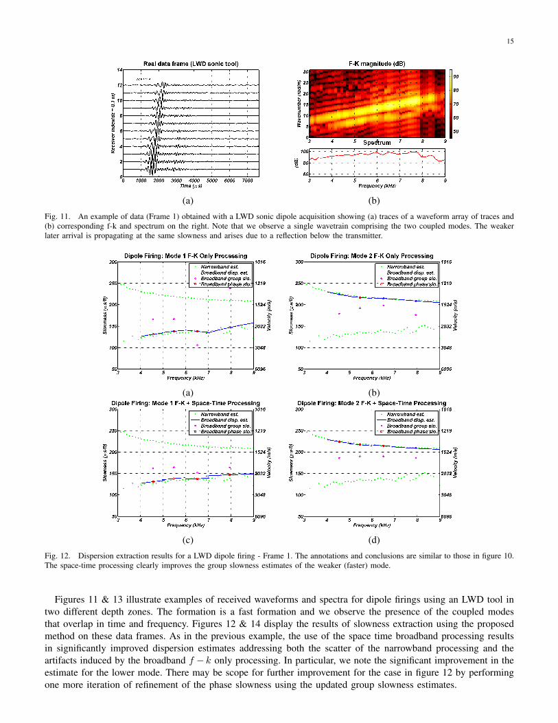
Fig. 11. An example of data (Frame 1) obtained with a LWD sonic dipole acquisition showing (a) traces of a waveform array of traces and(b) corresponding f-k and spectrum on the right. Note that we observe a single wavetrain comprising the two coupled modes. The weakerlater arrival is propagating at the same slowness and arises due to a reflection below the transmitter.

(a) (b)

(c) (d)

Fig. 12. Dispersion extraction results for a LWD dipole firing - Frame 1. The annotations and conclusions are similar to those in figure 10.The space-time processing clearly improves the group slowness estimates of the weaker (faster) mode.

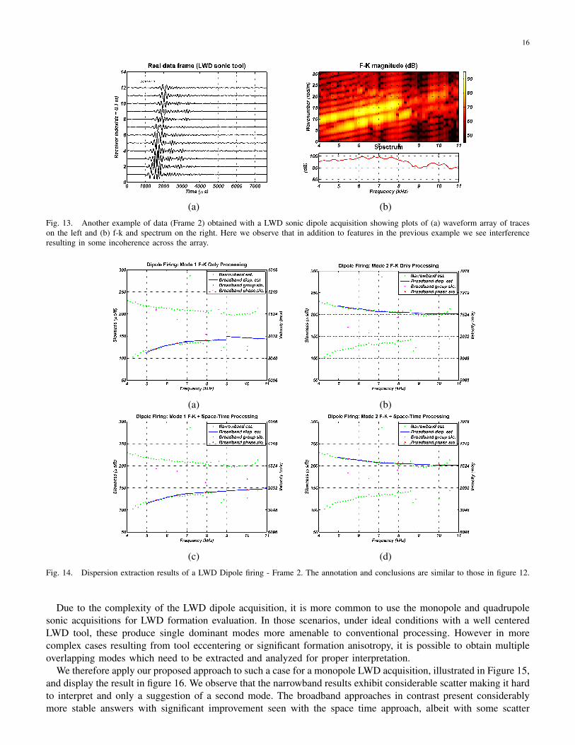
Figures 11 & 13 illustrate examples of received waveforms and spectra for dipole firings using an LWD tool intwo different depth zones. The formation is a fast formation and we observe the presence of the coupled modesthat overlap in time and frequency. Figures 12 & 14 display the results of slowness extraction using the proposedmethod on these data frames. As in the previous example, the use of the space time broadband processing resultsin significantly improved dispersion estimates addressing both the scatter of the narrowband processing and theartifacts induced by the broadband f − k only processing. In particular, we note the significant improvement in theestimate for the lower mode. There may be scope for further improvement for the case in figure 12 by performingone more iteration of refinement of the phase slowness using the updated group slowness estimates.

16

(a) (b)

Fig. 13. Another example of data (Frame 2) obtained with a LWD sonic dipole acquisition showing plots of (a) waveform array of traceson the left and (b) f-k and spectrum on the right. Here we observe that in addition to features in the previous example we see interferenceresulting in some incoherence across the array.

(a) (b)

(c) (d)

Fig. 14. Dispersion extraction results of a LWD Dipole firing - Frame 2. The annotation and conclusions are similar to those in figure 12.

Due to the complexity of the LWD dipole acquisition, it is more common to use the monopole and quadrupolesonic acquisitions for LWD formation evaluation. In those scenarios, under ideal conditions with a well centeredLWD tool, these produce single dominant modes more amenable to conventional processing. However in morecomplex cases resulting from tool eccentering or significant formation anisotropy, it is possible to obtain multipleoverlapping modes which need to be extracted and analyzed for proper interpretation.

We therefore apply our proposed approach to such a case for a monopole LWD acquisition, illustrated in Figure 15,and display the result in figure 16. We observe that the narrowband results exhibit considerable scatter making it hardto interpret and only a suggestion of a second mode. The broadband approaches in contrast present considerablymore stable answers with significant improvement seen with the space time approach, albeit with some scatter

17

(a) (b)

Fig. 15. An example of monopole data acquisition obtained with an LWD sonic tool showing plots of (a) waveform array of traces on theleft and (b) f-k and spectrum on the right. Note that the second mode, expected in this section traversing a bed boundary, is considerablyweaker than the first and is hidden in the sidelobes of the first on the f-k plot.

(a) (b)

(c) (d)

Fig. 16. Dispersion extraction results on a frame of LWD monopole sonic data. The annotation and conclusions are similar to those inthe figure 12. In this case, only the broadband approach is able to extract a dispersion curve for the weaker mode expected as explained infigure 15.

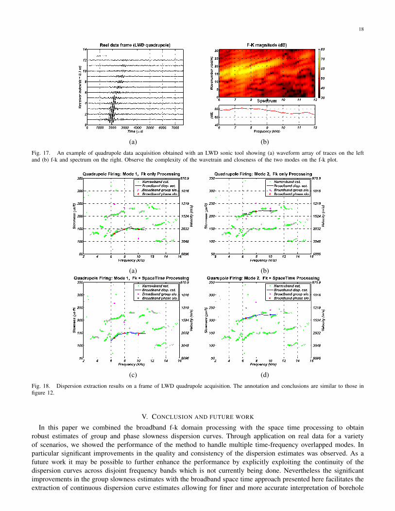
perhaps due to the challenging SNR environment.Finally we look at a case with an LWD quadrupole acquisition illustrated in figure 17 and show the results in

figure 18. Again the physical complexity results in the presence of two major overlapping modes whose dispersionsneed to be extracted for proper interpretation. The narrowband approach again yields a significant scatter of unlabeledpoint estimates. The broadband approach especially with the space-time processing results in much improveddispersion estimates that can be used for further analysis.

18

(a) (b)

Fig. 17. An example of quadrupole data acquisition obtained with an LWD sonic tool showing (a) waveform array of traces on the leftand (b) f-k and spectrum on the right. Observe the complexity of the wavetrain and closeness of the two modes on the f-k plot.

(a) (b)

(c) (d)

Fig. 18. Dispersion extraction results on a frame of LWD quadrupole acquisition. The annotation and conclusions are similar to those infigure 12.

V. CONCLUSION AND FUTURE WORK

In this paper we combined the broadband f-k domain processing with the space time processing to obtainrobust estimates of group and phase slowness dispersion curves. Through application on real data for a varietyof scenarios, we showed the performance of the method to handle multiple time-frequency overlapped modes. Inparticular significant improvements in the quality and consistency of the dispersion estimates was observed. As afuture work it may be possible to further enhance the performance by explicitly exploiting the continuity of thedispersion curves across disjoint frequency bands which is not currently being done. Nevertheless the significantimprovements in the group slowness estimates with the broadband space time approach presented here facilitates theextraction of continuous dispersion curve estimates allowing for finer and more accurate interpretation of borehole

19

acoustic data.

VI. APPENDIX

A. Cramer-Rao Bound for slowness estimation in f-k domain

Before we go into the details of the derivation of the Cramer Rao Bound (CRB) we would like to introducethe following notation. For a matrix A the transpose is denoted by AT and the conjugate is denoted by A∗. Theconjugate transpose is then denoted by (A∗)T . To this end recall that the Fisher Information Matrix J(Θ) as afunction of the parameters Θ is given by,

[J(Θ)]i,j = −E

{∂

∂θi∂θjlogP(Y|Θ)

}(32)

Then the CRB matrix is given by J−1. In the following we will derive general expressions for the various parts ofthe Fisher Information Matrix for the following set-up. The observations are obtained according to the observationmodel,

Y = AΘX + W (33)

where we assume that the noise W is i.i.d. complex Gaussian with zero mean and variance σ2 in each dimension.In our context Y ∈ CL.Nf×1 is the Fourier transform of the array data in the band F , AΘ denotes the arrayresponse (exponential) dependent on the real parameters Θ that capture the phase and the group slowness of themodes and X ∈ CM.Nf×1 is the mode spectrum corresponding to the M modes. We define the SNR as an overallSNR given by

SNR =||AΘX||22||W||22

(34)

Under this set-up the Log-Likelihood function LLΘ,X = logP(Y|Θ) as a function of (Θ,X) is given by

−LLΘ,X =1

σ2(Y∗ −A∗ΘX∗)T (Y −AΘX) + c (35)

=1

σ2(Y∗)TY − (X∗)T (A∗Θ)TY − (Y∗)TAΘX

+ (X∗)T (A∗Θ)TAΘX + c (36)

where the constant term c is only dependent on the noise variance σ2 and the dimension of the problem. In order toevaluate CRB the FIM has to be evaluated with respect to amplitudes |X| and the real parameters in Θ. Note thatthe derivative in equation 32 involve complex quantities. The common approach in this case is to represent eachquantity by its real and imaginary parts and take derivatives with respect to these. But more compact expressionsare obtained using sesquilinear convention. Such a form is suitable for real functions of complex quantities, e.g. Qand Q∗ (say) that can be expressed as functions of Q±Q∗ or (Q∗)TQ. For taking the derivatives we then simplyregard Q and Q∗ as independent variables and take derivatives with respect to them. One can then go back to thereal quantities by applying a suitable transformation.

Therefore in order to evaluate the CRB we evaluate the Fisher Information Matrix (FIM) with variables X,X∗,Θand where Θ is the vector of parameters that we are trying to estimate. In order to apply the sesquilinear conventionwe note that for a real function f(AΘ,A

∗Θ)

∂

∂θf(AΘ,A

∗Θ) =Tr

{(∂

∂AΘ

f(AΘ,A∗Θ)

)T ∂AΘ

∂θ

+

(∂

∂A∗Θf(AΘ,A

∗Θ)

)T ∂A∗Θ∂θ

}(37)

where Tr(.) is the Trace operation. In the following we will use the following standard conventions used for matrix

20

calculus - For matrices A,X,B

∂

∂XTr(AXB) = ATBT (38)

∂

∂XTr(AXTB) = BA (39)

Using the above relation we have,

−σ2 ∂

∂AΘLLΘ =

(−Y∗XT + A∗ΘX∗XT

)(40)

−σ2 ∂

∂A∗ΘLLΘ =

(−Y(X∗)T + AΘX(X∗)T

)(41)

This implies the following.

−σ2 ∂

∂θLLΘ,X =Tr

{(−X(Y∗)T + X(A∗ΘX∗)T

) ∂AΘ

∂Θ

+(−X∗YT + X∗(AΘX)T

) ∂A∗Θ∂θ

}(42)

After taking the derivative again with respect to θ we note that the terms involving double derivatives in AΘ

and A∗Θ evaluate to zero under the expectation operation. Therefore we have,

−σ2E

[∂2

∂θ2LLΘ,X

]=Tr

{X(X∗)T

(∂A∗Θ∂θ

)T ∂AΘ

∂θ

+ X∗XT

(∂AΘ

∂θ

)T ∂A∗Θ∂θ

}(43)

Now note that

−σ2 ∂

∂XLLΘ,X = −AT

ΘY∗ + ATΘA∗ΘX∗ (44)

This implies,

−σ2 ∂

∂X

∂

∂θLLΘ,X =(Y∗)T − (X∗A∗Θ)T

∂

∂θAΘ

+ ATΘ(∂A∗Θ∂θ

)T (X∗)T (45)

The above implies that

−σ2E

[∂

∂X

∂

∂θLLΘ,X

]= AT

Θ(∂A∗Θ∂θ

)T (X∗)T (46)

Using the above formulas it is easy to show that for all θi, θj ∈ Θ,

−σ2E∂

∂θiθjLLΘ,X =Tr

{X(X∗)T

∂(A∗Θ)T

∂θi

∂AΘ

∂θj

+ X∗(X)T∂(AΘ)T

∂θi

∂A∗Θ∂θj

}(47)

and for all θi ∈ Θ

−σ2E∂

∂X∗∂

∂θiLLΘ,X = (A∗Θ)T

∂AΘ

∂θiX (48)

−σ2E∂

∂X

∂

∂θiLLΘ,X = (AΘ)T

∂A∗Θ∂θi

X∗ (49)

21

AΘ =

vΘ1

(f1) vΘ2(f1)

vΘ1(f2) vΘ2

(f2). . . . . .

vΘ1(fNf ) vΘ2

(fNf )

(53)

−σ2 ∂

∂X∗∂

∂XLLΘ,X = AT

ΘA∗Θ (50)

−σ2 ∂

∂X

∂

∂X∗LLΘ,X = (A∗Θ)TAΘ (51)

B. Fisher Information for slowness estimation

We will use the general expressions derived above for finding the CRB for slowness estimation for a 2-modeproblem. To this end note that

Θ = [θ1, θ2, θ3, θ4] = [k1, k′

1, k2, k′

2] (52)

Also let Θ1 = [θ1, θ2] = [k1(f0), k′

1(f0)] and Θ2 = [θ3, θ4] = [k2(f0), k′

2(f0)] are the dispersion parameters forthe two modes. Following the formulation used before we define in this case the matrix AΘ is given by Equation53. where

vΘm(f) =

e−i2π(km+k

′m(f−f0))(z1−z0)

e−i2π(km+k′m(f−f0))(z2−z0)

...e−i2π(km+k

′m(f−f0))(zL−z0)

(54)

m = 1, 2, f ∈{f1, f2, ..., fNf

}. Then

−σ2E∂

∂θiθjLLΘ,X =Tr

{X(X∗)T

∂(A∗Θ)T

∂θi

∂AΘ

∂θj

+X∗(X)T∂(AΘ)T

∂θi

∂A∗Θ∂θj

}(55)

The above expression is equal to,

2 Tr Real

∑fi

X1(fi)X∗2(fi)

[∂

∂θi(B∗Θ(fi))

T ∂

∂θjBΘ(fi)

] (56)

where BΘ(f1) = [vΘ1(f1),vΘ2

(f1)] and X1,X2 ∈ CNf×1 are the coefficients of the mode spectrum for the twomodes. For the cross terms it can be shown that

(AΘ)T∂A∗Θ∂θi

X∗ =

[vTΘ1

∂v∗Θ1

∂θiX∗1(f1) + vTΘ1

∂v∗Θ2

∂θiX∗2(f1)

vTΘ2

∂v∗Θ1

∂θiX∗1(f1) + vTΘ2

∂v∗Θ2

∂θiX∗2(f1)

]......

(57)

and similar expressions can be obtained for the other term (A∗Θ)T ∂AΘ

∂θiX. Now note that for the particular choice

22

of z0 to be the median of the array locations z1, z2, ...zL the terms,

vTΘ1

∂v∗Θ1

∂θiX∗1(f1) = 0 (58)

vTΘ2

∂v∗Θ2

∂θiX∗2(f1) = 0 (59)

This means that the slowness estimates decouple from the amplitude estimates for each mode. However theinterference terms remain. For given values of the phase and group slowness and the mode spectrum one canthen calculate the CRB from the general expression for the FIM obtained above. In order to obtain the CRB interms of amplitudes and phase one simply applies the following transformation

KTFIMK (60)

where

K =

diag(

X|X|

)diag

(X∗

|X|

)0

idiag(X) −idiag(X∗) 00 0 I

(61)

to the FIM as obtained above using the sesquilinear analysis before taking the inverse. In the above equation diag(·)of a vector is a diagonal matrix with the diagonal being composed of the elements from the vector. Below we willderive simple error bounds to time location estimates using the error bounds on the phase location estimates.

C. Obtaining error bounds for time location estimates

One can use the error bounds on the phase estimates obtained from the CRB analysis above to obtain errorbounds on the time location estimates. Indeed in principle one may further parameterize the set-up in terms of thelinear phase of the mode spectrum but here we will take an alternate approach. We will essentially use the errorbound on the slope for the Least Squares Fit obtained from erroneous data , [27] to bound the error on the timelocation estimate. From CRB let the error variance in the phase estimates of the mode spectrum of a mode be givenby - e1, ..., eNf . Then the variance in the estimation of slope at points f1, ..., fNf is given by,

Var(slope) =es

esff(62)

where

es2 =1

Nf − 2

Nf∑i=1

e2i (63)

esff =

Nf∑i=1

(fi − f)2, f =1

Nf

Nf∑i=1

fi (64)

REFERENCES

[1] S. Aeron, S. Bose, H.-P. Valero, and V. Saligrama, “Broadband dispersion extraction using simultaneous sparse penalization,” IEEETransactions on Signal Processing, vol. 50, no. 10, pp. 4821–4837, 2011.

[2] F. L. Paillet and C. H. Cheng, Acoustic Waves in Boreholes. CRC Press, 1991.[3] B. Sinha, A. Norris, and S. Chang, “Borehole flexural modes in anisotropic formations,” Geophysics, vol. 59, pp. 1037–1052, 1994.[4] B. Sinha and S. Zeroug, Geophysical Prospecting Using Sonics and Ultrasonics, J. G. Webster, Ed. Wiley Interscience, 1999.[5] S. Lang, A. Kurkjian, J. McClellan, C. Morris, and T. Parks, “Estimating slowness dispersion from arrays of sonic logging waveforms,”

Geophysics, vol. 52, no. 4, pp. 530–544, April 1987.[6] M. P. Ekstrom, “Dispersion estimation from borehole acoustic arrays using a modified matrix pencil algorithm,” in 29th Asilomar

Conference on Signals, Systems and Computers, vol. 2, 1995, pp. 449–453.[7] B. Nolte and X. Huang, “Dispersion analysis of split flexural waves,” Massachusetts Institute of Technology, Tech. Rep., 1997.[8] X. M. Tang and C. Cheng, Quantitative borehole acoustic methods. Elsevier Science Publication Co., Inc., 2004.[9] V. N. R. Rao and M. N. Toksoz, “Dispersive wave analysis - method and applications,” MIT Earth Resources Laboratory, Tech. Rep.,

2005.[10] R. Roy and T. Kailath, “ESPRIT - estimation of signal parameters via rotational invariance techniques,” IEEE Transactions on Acoustics

Speech and Signal Processing, vol. 43, no. 7, pp. 984–995, July 1989.

23

[11] M. Viberg, “Subspace fitting concepts in sensor array processing,” PhD Thesis, Linkoping University, 1989.[12] M. Wax and T. Kailath, “Detection of signals by information theoretic criteria,” IEEE Transactions on Acoustics Speech and Signal

Processing, vol. 33, no. 2, pp. 387–392, April 1985.[13] J. Rissanen, “Modeling by shortest data description,” Automatica, vol. 14, pp. 465–471, 1978.[14] C. Wang, “Sonic well logging methods and apparatus utilizing parametric inversion dispersive wave processing,” US Patent, US7120541

B2, 2004.[15] A. Roueff, J. I. Mars, J. Chanussot, and H. Pedersen, “Dispersion estimation from linear array data in the time-frequency plane,” IEEE

Transactions on Signal Processing, vol. 53, no. 10, pp. 3738–378, October 2005.[16] S. Aeron, S. Bose, and H. P. Valero, “Automatic dispersion extraction using continuous wavelet transform,” in IEEE International

Conference on Acoustics, Speech and Signal Processing (ICASSP), Las Vegas, NV, 2008.[17] F. Auger and P. Flandrin, “Improving the reliability of time frequency time-scale representation by the reassignment method,” IEEE

Transactions on Signal Processing, vol. 43, no. 5, pp. 1068–1089, 1995.[18] W. H. Prossner and M. D. Seale, “Time frequency analysis of the dispersion of lamb modes,” Journal of Acoustical Society of America,

vol. 105, no. 5, pp. 2669–2676, May 1999.[19] K. Hsu, C. Esmersoy, and T. L. Marzetta, “Simultaneous phase and group slowness estimation of dispersive wavefields,” in Proc. th

Annual International Geoscience and Remote Sensing Symposium (IGARSS). ‘Remote Sensing Science for the Nineties’, 20–24 May1990, pp. 367–370.

[20] J. A. Tropp, “Just relax: Convex programming methods for identifying sparse signals,” IEEE Trans. Info. Theory, vol. 51, no. 3, pp.1030–1051, March 2006.

[21] C. Kimball and T. Marzetta, “Semblance processing of borehole acoustic array data,” Geophysics, vol. 49, no. 3, pp. 264–281, March1984.

[22] A. Kurkjian, “Numerical computation of the individual far-field arrivals excited by an acoustic source in a borehole,” Geophysics,vol. 50, pp. 852–866, 1985.

[23] J. A. Franco, M. M. Ortiz, G. S. De, L. Renlie, and S. Williams, “Sonic investigations in and around the borehole,” Oilfield Review,vol. Spring, 2006.

[24] A. Grossmann and J. Morlet, “Decomposition of Hardy functions into square integrable wavelets of constant shape,” SIAM Journal ofMathematical Analysis, vol. 15, pp. 723–736, 1984.

[25] A. Grossmann, R. Kornland-Martinet, and J. Morlet, Wavelet, Time-Frequency methods and phase space, ser. Reading and understandingcontinuous wavelet transform, J. Combes, A. Grossmann, and P. Tchamitchian, Eds. Springer-Verlag, Berlin, 1989.

[26] B. Sinha, E. Simsek, and S. Asvadurov, “Influence of a pipe tool on borehole modes,” Geophysics, vol. 74, no. 3, pp. E111–E123,2009.

[27] F. S. Acton, Analysis of Straight-Line Data. Dover, New York, 1966.