Embed Size (px)
Citation preview
1) Istituto Nazionale di Geofisica e Vulcanologia – Sezione Catania
2) GNS Science – New Zealand
USEReST, Naples, 11-13 November 2008
Currenti G.1, Del Negro C. 1, Scandura D. 1, Williams C.A. 2
Automated procedure for InSAR data
inversion using Finite Element Method

slipdisplacement Green’s function
Deformation model: Fault slip distribution
Dislocation source parameters determined from multiple types of static deformation data such as GPS displacements, InSAR imagery, and surface offset measurements suggest that slip along a fault is not uniform and is best described as a distribution of dislocation sources.
The procedure requires:1) subdividing the faults in a finite
number of patches;2) computing the Green's Function for
all the patches and the measurement points;
3) solving a linear inversion problem to determine the slip distribution.
jj
iji sGd
Gsd

26/5 pVE
]2)/(2/[]2)/[( 22 spsp VVVV
At each node of the mesh different values of Young modulus and Poisson ratio are assigned on the basis of seismic tomography investigations (Patanè et al., 2006).
Young modulus 11.5-133 GPa
Poisson ratio 0.12-0.32
FEM generated Green’s function
LaGritMesh refinement and smoothing are available to provide a mesh with more resolution in areas of interest.
www.meshing.lanl.gov
PyLithPyLith is a finite element parallel code for the solution of dynamic and quasi-static deformation problems.
www.geodynamcis.org
Medium Heterogeneity
Real Topography

MNMNN
MM
MM
sGsGd
sGsGd
sGsGd
11
21122
11111
System of linear equations
n x m patches
3 x n x m unknown variables!
(dip-slip, strike-slip, tensile)j ≥ 3 x n x m
FEM Inversion
Non-uniquiness of the solution can arise from limited data and poor knowledge of the internal structure. This issue can be faced using: (i) as much data as possible and (ii) numerical technique to reduce the algebraic ambiguity.

Geodetic Data Integration
)()(2
1minmin dsGWWdsG d
Td
Td
rd minmin
sG
G
d
d
GPS
SAR
GPS
SAR
M
MNNNN
MNNNN
MNNNN
MNN
MNN
MNN
MNMN
M
N
N
N
N
s
s
GG
GG
GG
GG
GG
GG
GG
GG
U
U
U
U
U
U
d
d
GSGS
GSGS
GSGS
SS
SS
SS
SS
G
z
G
y
G
x
z
y
x
S
S
1
,31,3
,131,13
,231,23
,31,3
,21,2
,11,1
,,
,11,1
1
1
1
1
Linear least-squares methods for this problem require to incorporate regularization techniques in order to stabilize the problem and to reduce the set of likely solution.
EDM, GPS, leveling data assure high measurements accuracy but the coverage area is usually limited. InSAR data, despite the lower accuracy, can provide a better overview of the deformation pattern thanks to the wide coverage.
A Wd covariance matrix is introduced to weight the data depending on measurements uncertainties.

UsLWsWsdsGWWdsG
,)()(2
1minmin TT
dTd
T
The inverse problem can be re-formulated as an optimization problem aimed at finding the unknown slip values s that minimize a data misfit and a smoothing functional:
As smoothing functional, the Laplacian Operator was used to avoid large variations between neighboring dislocations.
FEM Inversion & Regularization
The minimization of the quadratic functional φ subjected to bound constraints can be solved by using a Quadratic Programming algorithm based on an active set strategy (Gill et al., 1991):
WWGWWGQ Td
Td
T dWWGb dTd
T
UsLsbsQs
,2
1minmin TT
where:

φd
φw
The L-curves of the data misfit versus the model norm as a function of the regularization parameter. The best value of regularization parameter lies on the corner of the L-curve.
Input Fault Slip Distribution
L-curve criterion

s
1 – Domain and Fault discretization:
LaGrit
2 – FEM generated Green’s function: PyLith 3 – Solving a
linear inversion problem: QP algorithm
Procedure Scheme
Ground deformation data (SAR, GPS,
EDM)

Analytical vs Numerical Solution
Simulat. # 1 # 2 # 3 # 4 # 5 # 6 # 7 # 8
Nodes 2228 2513 2570 3195 3977 5101 8591 36196
Elements 9858 11236 11505 14663 18888 25141 4502120570
0
Quality 0.3544 0.3083 0.3441 0.3109 0.3417 0.2960 0.3050 0.2454
We considered a 3D FEM model reproducing a rectangular dislocation source in a homogeneous and isotropic half-space and compare it with the Okada’s solution.
N
i
N
i
ANi
ANi
FEii UUUU
1 1
/)(
A misfit index was used to quantify the discrepancy between the numerical and the analytical solution:
Currenti et al. PEPI 2008
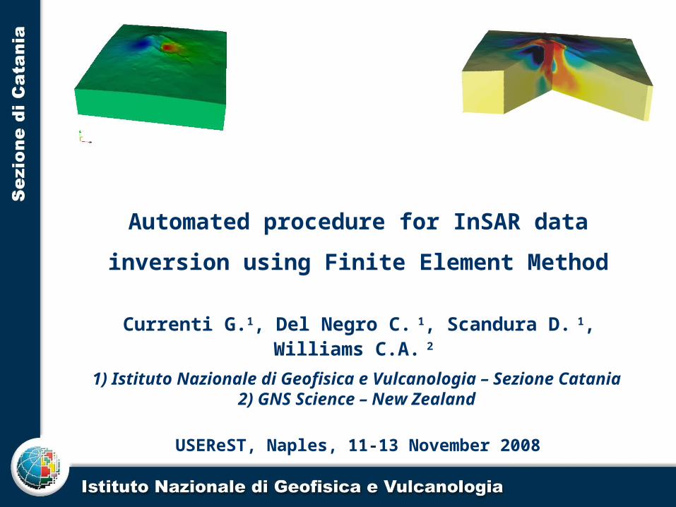
Tests on the Accuracy
We compare the ground deformation achieved as the sum of the displacements generated by each patch and those obtained by the overall fault. In these computations a uniform slip distribution on the patch is assumed. The error has a RMSE (root mean square error) of the order of 10-7 m, which is well below the measurement error.
The accuracy of the solution is dependent on the number of the observation points. A uniform distribution of observation points within a regular grid was assumed, centered on the ground projection of the sources. The RMSE between the assumed and the inverted slip is computed as the number of measurement points increases.
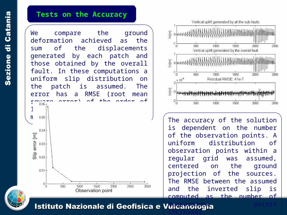
Differential interferogram for ascending scene pair 31 July 2002 to 09 October 2002. The scale indicates the phase variation along the LOS (negative values correspond to the approaching of the surface to the sensor)
Bonforte et al., Bull Volc. 2007
On 22 September 2002, 1 month before the beginning of the flank eruption on the NE Rift, an M-3.7 earthquake struck the northeastern part of Mt. Etna, on the westernmost part of the Pernicana fault.
A case study: Northeastern flank movement at Etna volcano in 2002
The GPS surveys carried out in September and July 2002 shows a ground deformation pattern that affects the northeastern flank clearly shaped by the Pernicana fault.
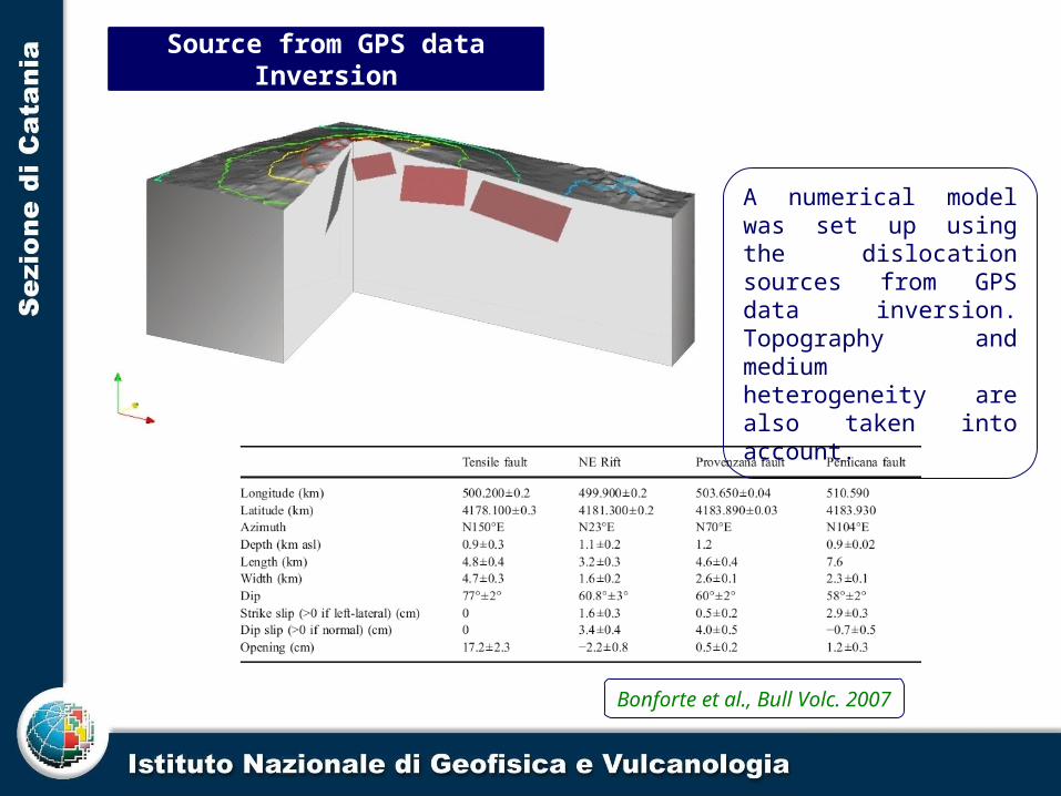
Source from GPS data Inversion
Bonforte et al., Bull Volc. 2007
A numerical model was set up using the dislocation sources from GPS data inversion. Topography and medium heterogeneity are also taken into account.

3D FEM of Mt. Etna: slip on Northeastern Flank
Computing Time: 15 minutes
Mesh Domain:100 x 100 x 50 kmNodes: 129253Tetrahedra Elements: 744886

Sar Data and Source Discretization
A deformation pattern is clearly seen around the Pernicana volcano edifice structure.
Line of sight change map calculated by the unwrapped interferograms, processed using ROI_PAC software, developed by Jet Propulsion Laboratory & Caltech; Courtesy of F. Guglielmino ed A. Spata. The dislocation sources were
subdivided in patches to obtain the slip distribution from the inversion procedure.

Green Functions Computations
248 fault patches
248 x 3 = 744 FEM simulations
21 87 744
FEM simulations
By a linear speedup on a cluster of 20 nodes the computing time reduces from 10 days to 10 hours.
Dip-slip, strike-slip and tensile dislocation were assigned to the nodes lying along the fault surface. For each patches, in which the fault is discretized, Green’s functions were computed using PyLith. For each each simulations, the accuracy was warranted checking the convergency of the FEM solution. The iteration of GMRES solver is stopped when a threshold of 10-9 is reached or the number of iterations is higher than 200.

Inversion Results
0 1 2 3 4 5 6 7
x 10-9
16
16.5
17
17.5
18
18.5
19
1000
Smoothing Functional
Dat
a M
isfit
SAR data
The kinematic of the faults was constrained to those derived from GPS data inversion. The solution in correspondence of the corner of the L-curve provides a deformation pattern which resembles the SAR data and also matches the GPS obtained from the analytical solution.
Inverted Solution

Slip Distribution
Strike-slip, dip-slip and tensile dislocation distribution.

Model Comparison
The GPS data inversion provides a deformation pattern which misses the clear anomaly around the Pernicana fault system. A heterogeneous distribution of the slip along the structure is able to better justify the SAR data. The FEM model based on the numerical inversion provides a more complex pattern which is likely to be expected.SAR data
Analytical Model Numerical Model

An automated procedure for geodetic data inversion is proposed to estimate slip distribution along fault interfaces. 3D finite element models (FEMs) are implemented to compute synthetic Green’s functions for static displacement.
Conclusions
The procedure was applied to study the ground deformation preceding the 2002-03 Etna eruption. SAR images showed a significant deformation pattern of the north-eastern flank of the volcano involving the main local volcanic edifice features on the northeastern flank. The numerical model highlighted a heterogeneity slip distribution along the Pernicana fault with a predominant strike-slip mechanism associated with a dip-slip movement in the western part.
FEM-generated Green’s functions computed using PyLith, a source-free parallel finite element code, are combined with a Quadratic Programming algorithm to invert ground deformation data and obtain an estimate of slip distributions along seismogenic structures.
The time consuming computation of the procedure is related to the generation of the Green’s functions. For the main volcano edifice features and the seismogenic structures they has to be computed only once and stored in a database.

Numerical Solution
Currenti et al. PEPI 2008
Several computations were performed to better understand the effects induced by the topography and the medium heterogeneity. The topography significantly alters the general pattern of the ground deformation especially near the volcano summit. On the contrary, the medium heterogeneity does not strongly affect the expected deformation.

The Laplacian Operator is introduced to avoid large variations between neighboring dislocations
The matrix WL is constructed so that the n-th row in WL contains coefficients in the equation above for columns corresponding to the neighboring source.
2
2)2(
2)1()1(
2)1()1(
22)1( 2
yW
yW
xW
xW
yxW
W
ijnc
incj
incj
incj
incj
L
2
1,,1,
2
,1,,12
)(
2
)(
20
y
sss
x
ssss jijijijijiji
Smoothing Functional
)()()()(2
1min 00 ssWWssdsGWWdsG L
TL
Td
Td
T
sWWsdsGWWdsG L
TL
Td
Td
T )()(2
1min