Embed Size (px)
Citation preview

The First Derivative of Ramanujans Qubic Continued Fraction
Nikos BagisDepartment of Informatics
Aristotele University of Thessaloniki [email protected]
Abstract
We give the complete evaluation of the first derivative of theRamanujans qubic continued fraction using Elliptic functions.The Elliptic functions are easy to handle and give the resultsin terms of Gamma functions and radicals from tables. Theresults appear to be new.
keywords Jacobian Elliptic Functions; Continued Fractions; Ra-manujan; Qubic Fraction; Derivative
1 Introduction
The Ramanujan’s Cubic Continued Fraction is (see [3], [7], [8], [9], [11]).
V (q) :=q1/3
1+q + q2
1+q2 + q4
1+q3 + q6
1+. . . (1)
Our main result is the evaluation of the first derivative of Ramanuajan’s qubicfraction. For this, we follow a different way from previous works and use thetheory of Elliptic functions, which is more easy to handle. Our method consiststo find the complete polynomial equation of the Qubic fraction in terms only ofthe inverse elliptic nome kr, which is a solvable, in radicals, quartic equation.Using the derivative of kr which we evaluate in Section 2 of this article, we findthe desired formula.We give some definitions firstLet
(a; q)k =k−1∏n=0
(1− aqn) (2)
Then we definef(−q) = (q; q)∞ (3)
andΦ(−q) = (−q; q)∞ (4)
Also let
K(x) =∫ π/2
0
1√1− x2 sin2(t)
dt (5)
1

be the elliptic integral of the first kind.We denote
θ4(u, q) =∞∑
n=−∞(−1)nqn
2e2nui (6)
the Elliptic Theta function of the 4th-kind.∞∏n=1
(1− q2n)6 =2kk′K(k)3
π3q1/2(7)
and from
q1/3∞∏n=1
(1 + qn)8 = 2−4/3
(k
1− k2
)2/3
(8)
we get
f(−q)8 =∞∏n=1
(1− qn)8 =28/3
π4q−1/3k2/3(k′)8/3K(k)4 (9)
The variable k is defined from the equation
K(k′)K(k)
=√r (10)
where r is positive , q = e−π√r and k′ =
√1− k2. Note also that whenever r is
positive rational, the k are algebraic numbers.For the above one can see and [15].
2 The Derivative {r, k}Lemma 1. If |t| < πa/2 and q = e−πa then
∞∑n=1
cosh(2tn)n sinh(πan)
= log(f(−q2))− log(θ4(it, e−aπ)
)(11)
Proof. From the Jacobi Triple Product Identity (see [4]) we have
θ4(z, q) =∞∏n=0
(1− q2n+2)(1− q2n−1e2iz)(1− q2n−1e−2iz) (12)
By taking the logarithm of both sides and expanding the logarithm of the indi-vidual terms in a power series it is simple to show (17) from (18).
Lemma 2.Let q = e−π
√r
φ(x) = 2d
dx
(∂
∂tlog(ϑ4
(itπ
2, e−2πx
))t=x
)(13)
2

thend(√r)
dk=
K(1)(k)
φ(K(√
1−k2)K(k)
) =K(1)(k)
φ(K(k′)K(k)
) (14)
Where K(1)(k) is the first derivative of K.Proof. From Lemma 1 we have
2∂
∂tlog(ϑ4
(itπ
2, e−2πx
))t=x
= −π∞∑n=1
1cosh (nπx)
=π
2−K(kx)
then √x(k2)−
√x(k1) = −
∫ k2
k1
K(1)(k)
φ
(K(√
1−k2)K(k)
)dkDifferantiating the above relation with respect to k we get the result.
Lemma 3. Set q = e−π√r and
{r, k} :=dr
dk= 2
K(k′)K(1)(k)
K(k)φ(K(k′)K(k)
)Then
{r, k} =πK ′
K2
1−5k2
k−k3 + 6K(1)
K
(k2 − 5)K + 6E(15)
Proof. From (9) taking the logarithmic derivative with respect to k and usingLemma 2 we get:
π {r, k}
(1− 24
∞∑n=1
nqn
1− qn
)=(
1− 5k2
(k − k3)+
6K(1)
K
)4K ′
K(16)
But it is known that∞∑n=1
nqn
1− qn=
124
+K
6π2((5− k2)K − 6E) (17)
From the above relations we get the result.Note.1) The first derivative of K is
K(1) =E
k · k′2− K
kr
where k = kr and k′ = k′r =√
1− k2r .
2) In the same way we can find form the relation
k4r =1− k′r1 + k′r
(18)
3

the modular equation of 2-degree derivative.Noting first that (the proof is easy):
{r, k′r} =k′rkr{r, kr} (19)
we have
{r, k4r} =k′r(1 + k′r)
2
2kr{r, kr} (20)
3 The Ramanujan’s Cubic Continued Fraction
Let
V (q) :=q1/3
1+q + q2
1+q2 + q4
1+q3 + q6
1+. . . (21)
is the Ramanujan’s cubic continued fraction, then
Lemma 4.
V (q) =2−1/3(k9r)1/4(k′r)
1/6
(kr)1/12(k′9r)1/2(22)
where the k9r are given by (see [7]):√krk9r +
√k′rk′9r = 1 (23)
Proof. It is known (see and [12] pg. 596) that
V (q) = q1/3(q; q2)∞(q3; q6)3∞
ButΦ(−q) = (−q, q)∞ =
1(q, q2)∞
thus
V (q) = q1/3Φ(−q3)3
Φ(−q)and equation (19) follows from (8).
Lemma 5.If
G(x) =x√
2√x− 3x+ 2x3/2 − 2
√x√
1− 3√x+ 4x− 3x3/2 + x2
andkr = G(w) (24)
4

thenk9r =
w
kr
and
k′9r =(1−
√w)2
k′r
Proof. Set the values of kr and k9r in (20).If we set
W = 2− 3√w + 2w − 2(1−
√w)√
1−√w + w (25)
then
V (q) =(k′r)
2/3w1/4
21/3(kr)1/3(1−√w)
=(W − w3/2)1/3W−1/6
21/3(1−√w)
(26)
after solving (22) with respect to w and making the simplifications we arrive at
2V 3(q) =√W
(1 +√W )2
(27)
and
(kr)2 =√W
(2 +√W
1 + 2√W
)3
(28)
Hence we get the following equation
(kr)2/3 = Z2
√2V (q)3/2 + Z3
−√
2V (q)3/2 + 2Z3(29)
Where Z = 12√W (q). Reducing the above equation in polynomial form we have
sk2/3r + sZ2 − 2k2/3
r Z3 + Z5 = 0 (30)
and
s2 = 2V 3(q) =Z6
(1 + Z6)2(31)
From these two equations we arrive to
Theorem 1. Set T =√
1− 8V 3(q) then
(kr)2 =(1− T )(3 + T )3
(1 + T )(3− T )3(32)
Equation (29) is a solvable quartic equation with respect to T .An example of evaluation is
V (e−π) =12
(−2−
√3 +
√3(3 + 2
√3))
(33)
5

Main Theorem.
V ′(q) = −23
V (q) + V 4(q)kr {r, k}
√1− 8V 3(q)
(34)
The derivative {r, k} is given form (15).Proof. Derivate (32) with respect to r then√
2kr{k, r}
=4T (3 + T )
(3− T )2(1 + T )
√dT
dr(35)
or
Tr =dT
dr=
18kr {r, k}
(9− T 2)(1− T 2)T 2
(36)
Using the relation T =√
1− 8V (q)3, we get the result.
We use oftenly the notations V [r] := V (e−π√r), T [r] := T (e−π
√r).
Proposition.
V [4r] =1− T [r]
4V [r](37)
Proof. From (18) and Theorem 1 we get the result using simplifications withMathematica. For a more completed proof see [9].
Proposition.
T ′[4r]T ′[r]
=(1− T [r])(3 + T [r])
8√T [r](1 + T [r])5/3(3− T [r])1/2
(38)
Proof. From (18), (19), (20) and (34) we get
V ′[4r] =−2 {k, r}
3 1−k′
1+k′k′(1+k′)2
2k
V [4r] + V [4r]4
T [r](39)
If we use the duplication formula (37) we get the result.
Note.1) We can calculate now easy the values of V ′(q) from (31) using (29) and (15).An example of evaluation is
k1 =1√2
6

,
E(k1) =4π3/2
Γ(−1/4)2+
Γ(3/4)2
2√π
and
K(k1) =8π3/2
Γ(−1/4)2
When r = 1 we get
{r, k} =8√
2Γ(3/4)4
π2
Hence
V ′(e−π) = −
√6(12 + 7
√3)− 6− 3
√3
24Γ(3/4)4π2 (40)
2) It is
T1 = T (e−π√
3) = −39 + 22√
3− 2 · 62/3(−123 + 71√
3)(−4725 + 2728
√3−
√4053− 2340
√3)1/3
+
+2 · 61/3
(−4725 + 2728
√3−
√4053− 2340
√3)1/3
and V1 = V (e−π√
3) = 12
3√
1− T 21 .
From tables it is:
{3, k3} =96 · 21/3πΓ(2/3)2
(21/3√
3Γ(1/3)4 − 16(3 + 2√
3)πΓ(2/3)2)√
2−√
3((3 + 2
√3)Γ(1/3)8 − 96 · 22/3(12 + 7
√3)π3Γ(4/3)2
)We find the value of V ′(e−π
√3) in terms of Gamma function and algebraic
numbers.
V ′(e−π√
3) = −23
V1 + V 41
k3 {3, k3}√
1− 8V 31
3) Solving (36) with respect to T we get
T =
√5− 4cTr +
12
√−36 + (−10 + 8cTr)2 (41)
Where c = {r, k} kr
7

References
[1]: M.Abramowitz and I.A.Stegun. ’Handbook of Mathematical Functions’.Dover Publications, New York. 1972.
[2]: C. Adiga, T. Kim. ’On a Continued Fraction of Ramanujan’. TamsuiOxford Journal of Mathematical Sciences 19(1) (2003) 55-56 Alethia University.
[3]: C. Adiga, T. Kim, M.S. Naika and H.S. Madhusudhan. ’On Ramanu-jan‘s Cubic Continued Fraction and Explicit Evaluations of Theta-Functions’.arXiv:math/0502323v1 [math.NT] 15 Feb 2005.
[4]: G.E.Andrews. ’Number Theory’. Dover Publications, New York. 1994.[5]: B.C.Berndt. ’Ramanujan‘s Notebooks Part I’. Springer Verlang, New
York (1985).[6]: B.C.Berndt. ’Ramanujan‘s Notebooks Part II’. Springer Verlang, New
York (1989).[7]: B.C.Berndt. ’Ramanujan‘s Notebooks Part III’. Springer Verlang, New
York (1991).[8]: Bruce C. Berndt, Heng Huat Chan and Liang-Cheng Zhang. ’Ramanu-
jan‘s class invariants and cubic continued fraction’. Acta Arithmetica LXXIII.1(1995).
[9]: Heng Huat Chan. ’On Ramanujans Cubic Continued Fraction’. ActaArithmetica. 73 (1995), 343-355.
[10]: I.S. Gradshteyn and I.M. Ryzhik. ’Table of Integrals, Series and Prod-ucts’. Academic Press (1980).
[11]: Megadahalli Sidda Naika Mahadeva Naika, Mugur Chinna Swamy Ma-heshkumar, Kurady Sushan Bairy. ’General Formulas for Explicit Evaluationsof Ramanuajn‘s Cubic Continued Fraction’. Kyungpook Math. J. 49 (2009),435-450.
[12]: L. Lorentzen and H. Waadeland. ’Continued Fractions with Applica-tions’. Elsevier Science Publishers B.V., North Holland (1992).
[13]: S.H.Son. ’Some integrals of theta functions in Ramanujan’s lost note-book’. Proc. Canad. No. Thy Assoc. No.5 (R.Gupta and K.S.Williams, eds.),Amer. Math. Soc., Providence.
[14]: H.S. Wall. ’Analytic Theory of Continued Fractions’. Chelsea Publish-ing Company, Bronx, N.Y. 1948.
[15]:E.T.Whittaker and G.N.Watson. ’A course on Modern Analysis’. Cam-bridge U.P. (1927)
[16]:I.J. Zucker. ’The summation of series of hyperbolic functions’. SIAM J.Math. Ana.10.192 (1979)
8

Some Notes On a Continued Fraction of Ramanujan
Nikos BagisDepartment of Informatics
Aristotele University of Thessaloniki [email protected]
UNFINISHED
Abstract
Abstract
keywords Jacobian Elliptic Functions; Continued Fractions; Ra-manujan;
1 Introduction
Let
(a; q)k =k−1∏n=0
(1− aqn) (1)
Then we definef(−q) = (q; q)∞ (2)
andΦ(−q) = (−q; q)∞ (3)
Also let
K(x) =∫ π/2
0
1√1− x2 sin2(t)
dt (4)
be the elliptic integral of the first kindWe denote
θ4(u, q) =∞∑
n=−∞(−1)nqn
2e2nui (5)
the Elliptic Theta function of the 4th-kind.
∞∏n=1
(1− q2n)6 =2kk′K(k)3
π3q1/2(6)
and from
q1/3∞∏n=1
(1 + qn)8 = 2−4/3
(k
1− k2
)2/3
(7)
we get
f(−q)8 =∞∏n=1
(1− qn)8 =28/3
π4q−1/3k2/3(k′)8/3K(k)4 (8)
1

The variable k is defined from the equation
K(k′)K(k)
=√r (9)
where r is positive , q = e−π√r and k′ =
√1− k2. Note also that whenever r is
positive rational, the k are algebraic numbers.In Berndt’s book: Ramanujan’s Notebook Part III, ([B3] pg.21), one can
find the following expansion
Theorem 1. Suppose that either q, a and b are complex numbers with |q| < 1,or q, a, and b are complex numbers with a = bqm for some integer m. Then
U = U(a, b; q) =(−a; q)∞(b; q)∞ − (a; q)∞(−b; q)∞(−a; q)∞(b; q)∞ + (a; q)∞(−b; q)∞
=
a− b1− q+
(a− bq)(aq − b)1− q3+
q(a− bq2)(aq2 − b)1− q5+
q2(a− bq3)(aq3 − b)1− q7+
. . . (10)
Suppose now
X =(−a; q)∞(b; q)∞(a; q)∞(−b; q)∞
(11)
Then holdsX − 1X + 1
= U (12)
Corollary. Set
φ(q) =∞∑
n=−∞qn
2(13)
thenφ(q)− 1φ(q) + 1
=q
1 + q
−q3
1 + q3+−q5
1 + q5+−q7
1 + q7. . . (14)
Proof. Take q → q2 in (12) and then set a→ q and b→ q2.
Corollary.
Φ(−q)− f(−q)Φ(−q) + f(−q)
=q
1− q+q3
1− q3+q5
1− q5+q7
1− q7. . . (15)
Proof. Set b = 0 in (12) and then a = q.
2

Corollary.Φ(−q)− f(−q)Φ(−q) + f(−q)
= −φ(−q)− 1φ(−q) + 1
(16)
Proof. It follows from Corollary’s 1, 2
Proposition 1.
∞∑n=0
qn
1− a2q2n=
11− q+
−a2(1− q)2
1− q3+−qa2(1− q2)2
1− q5+−q2a2(1− q3)2
1− q7+. . . (17)
Proof. Divide relation (12) by a− b and then take the limit b→ a.
Corollary.
K(kr)2π
+14
=1
1− q+(1− q)2
1− q3+q(1− q2)2
1− q5+q2(1− q3)2
1− q7+. . . (18)
Proof. Set in (19) a = i, and q = e−π√r.
Now set
u(a, q) =2a
1− q+a2(1 + q)2
1− q3+a2q(1 + q2)2
1− q5+a2q2(1 + q3)2
1− q7+. . . (19)
and
P =(
(−a; q)∞(a; q)∞
)2
(20)
ThenP − 1P + 1
= u(a, q) (21)
or
Proposition 2.((−a; q)∞(a; q)∞
)2
= −1 +2
1−2a
1− q+a2(1 + q)2
1− q3+a2q(1 + q2)2
1− q5+a2q2(1 + q3)2
1− q7+. . .
(22)
Taking the logarithms in both sides of (24), we get easily as in Lemma 1 :
3
Proposition 3.
4∞∑n=0
a2n+1
(2n+ 1)(1− q2n+1)= log
(−1 +
21− u(a, q)
)(23)
Here we must mention that hods the more general formula (the proof is as inProposition 2)
2∞∑n=0
a2n+1 − b2n+1
(2n+ 1)(1− q2n+1)= log
(−1 +
21− U(a, b; q)
)(24)
Thus (−1 +
21− U(a, b; q)
)2
=
(−1 + 2
1−u(a,q)
)(−1 + 2
1−u(b,q)
) (25)
and for to study U we have to study only u.
Corollary.∫ q
0
11− x+
−x(1− x)2
1− x3+−x2(1− x2)2
1− x5+x3(1− x3)2
1− x7+. . . dx =
=14
log(−1 +
21−
2√q
1− q+q(1 + q)2
1− q3+q2(1 + q2)2
1− q5+. . .
)(26)
Proof. Differentiate with respect to a the relation (25) and use (19). Afterthat integrate to get the desired result.In some cases the u fraction can calculated in terms of elliptic functions. Forexample:
−1 +2
1− u(q, q)=
π
2k′rK(kr)(27)
In general holds
4∞∑n=0
qν(2n+1)
(2n+ 1)(1− q2n+1)= −4
ν−1∑j=1
arctanh(qj)− log(
2k′rK(kr)π
)from which we lead to the following:
Proposition 4.
−1+2
1− u(qν , q)= −1+
21−
2qν
1− q+q2ν(1 + q)2
1− q3+q2ν+1(1 + q2)2
1− q5+q2ν+2(1 + q3)2
1− q7+. . . =
4

=π
2k′rK(kr)exp
−4ν−1∑j=1
arctanh(qj)
(28)
Proposition 5.
−1 +2
1− U(qν1 , qν2 , q)= exp
−2
ν1−1∑j1=1
arctanh(qj1)−ν2−1∑j2=1
arctanh(qj2)
(29)
Proof. The proof follows easily from (25), (26) and (27) and (30).
Another formula related with u continued fraction is
−1 +2
1− u(qν+1/2, q)= exp
(−4
∞∑n=0
q(2n+1)(ν+1/2)
(2n+ 1)(1− q2n+1)
)
= exp
−4ν−1∑j=0
arctanh(qj+1/2) + arctanh(kr)
Hence also
kr = tanh
4ν−1∑j=0
arctanh(qj+1/2) + log(−1 +
21− u(qν+1/2, q)
) (30)
For every ν positive integer.Hence we obtain a continued fraction for kr
k′r1− kr
= −1 +2
1− u(q1/2, q)(31)
Inspired from the above relations and Propositions we have
Proposition 6.(Unproved)If c is positive real and ν1, ν2 positive integers then:
−1 +2
1− U(qν1+c, qν2+c, q)?=
= exp
−2
ν1−1∑j1=1
arctanh(qj1+c)−ν2−1∑j2=1
arctanh(qj2+c)
(32)
5

Also we observe that holds and(−1 +
21− U(a,−b; q)
)2?=(−1 +
21− u(a, q)
)(−1 +
21− u(b, q)
)(33)
This relation is similarly to (27). We also get the following unproved
Corollary.(Unproved)Let w ∈ Im(C), then∣∣∣∣−1 +
21− U(qν1+c,−wqν2+c, q)
∣∣∣∣ ?=(−1 +
21− u(qν1+c, q)
)(34)
Seting c = 0 in (35) and using Proposition 3 we get
Corollary. When w, z ∈ Im(C) and q = e−π√r, r > 0, then
(i)
∣∣∣∣−1 +2
1− U(qν1 ,−wqν2 , q)
∣∣∣∣ =π
2k′rK(kr)exp
−4ν1−1∑j=1
arctanh(qj)
(ii) ∣∣∣∣−1 +
21− U(−zqν1+c,−wqν2+c, q)
∣∣∣∣ = 1
We write (26) as
log(−1 +
21− U(a, b, q)
)= 2
∞∑n=1
an − bn
n(1− qn)−∞∑n=1
a2n − b2n
n(1− q2n)=
= 2∞∑n=1
(aq−1/2)n − (bq−1/2)n
n(q−n/2 − qn/2)−∞∑n=1
(aq−1/2)2n − (bq−1/2)2n
n(q−n − qn)
Set now b = e−v−2t, q = e−2t, a = ev then
log(−1 +
21− U(a, b, q)
)= log
(−1 +
21− U(ev, e−v−2t, e−2t)
)=
= 2∞∑n=1
e(v+t)n − e−(v+t)n
n(etn − e−tn)−∞∑n=1
e2(v+t)n − e−2(v+t)n
n(e2tn − e−2tn)=
6

= 2∞∑n=1
sinh((v + t)n)n sinh(tn)
−∞∑n=1
sinh(2(v + t)n)n sinh(2tn)
(a)
Set
U1(t) := limh→0
(−1 +
21− U(e−t+h, e−t+h, e−2t+h)
)(35)
Hence we get the following
Proposition 7.
d2ν+1
dt2ν+1log(U1(t)) = 2
∞∑n=1
n2ν+1
n sinh(tn)− 2
∞∑n=1
(2n)2ν+1
n sinh(2tn)(36)
Proof. Use Lemma and proceed derivating relation (a). Everytime take thelimit v → −t.
Corollary.
− d
dtlog (U1(t)) = − log(U1(t+ dh))
dh= 2
∞∑n=0
1sinh(t(2n+ 1))
(37)
Proof. Set ν = 0 in Proposition.
LemmaU1(t+ dh)ν − U1(t+ dh)−ν
2νdh?=
log(U1(t+ dh))dh
(38)
Lemma
F (U1(t+ dh))− F(U1(t+ dh)−1
)2dh
?= F ′(1)log(U1(t+ dh))
dh(39)
Proposition 8. For arbitrary non costant analytic functions Fj define TFj (x) =log(Fj(x)), j = 1, 2, . . . then
TFm◦ . . .︸︷︷︸
m
◦TF1(log(U1(x+ dh)))
dh= 2
∞∑n=0
1sinh((2n+ 1)x)
(40)
7

References
[1]:G.E.Andrews, Number Theory. Dover Publications, New York[2]:T.Apostol, Introduction to Analytic Number Theory. Springer Verlang,
New York[3]:M.Abramowitz and I.A.Stegun, Handbook of Mathematical Functions.
Dover Publications[4]:B.C.Berndt, Ramanujan‘s Notebooks Part I. Springer Verlang, New York
(1985)[5]:B.C.Berndt, Ramanujan‘s Notebooks Part II. Springer Verlang, New
York (1989)[6]:B.C.Berndt, Ramanujan‘s Notebooks Part III. Springer Verlang, New
York (1991)[7]:L.Lorentzen and H.Waadeland, Continued Fractions with Applications.
Elsevier Science Publishers B.V., North Holland (1992)[8]:E.T.Whittaker and G.N.Watson, A course on Modern Analysis. Cam-
bridge U.P. (1927)
8

1
Infinite Series and Divisor Sums
�ikos Bagis
Department of Informatics
Aristotle University of Thessaloniki
Thessaloniki Greece
SUBMITTED
Abstract
In this work we present and prove formulas having infinite and finite parts. The finite
parts are divisor sums which already known from the ancient Greeks. These sums can
lead us to very interesting formulas when attached to infinite expressions.
§1.General Theorems on Series
Proposition 1. If a, b are positive real numbers and f is analytic in (-1,1) with
(0) 0f = , then
( ) (0)1( )
!
1
(1 )
x dt
d n
f nf e dt
n d dnx
n
e e
µ−
∞
∞
−
=
∑∫= −∏ : (1)
Where µ is the Moebius function i.e.:
1 if 1
( ) ( 1) , if is the product of r discrete primes
0 else
r
k
k kµ=
= −
For the Moebius Function one can see [Ap].
Proof. Because f (0) = 0 and f analytic in (-1,1), the integral ( )
x
tf e dt−
∞∫ exists for
every x > 0. We assume that exists sequence X(n) such that:
( )( )
1
(1 )
x
tf e dtnx X n
n
e e
−
∞
∞−
=
∫= −∏

2
( )1
( ) ( ) log 1
x
t nx
n
f e dt X n e∞
− −
=∞
= −∑∫ =1 1
( )knx
n k
eX n
k
−∞ ∞
= =
−∑ ∑ =1 1
( )knx
n k
eX n n
kn
−∞ ∞
= =
−∑∑
1
( )nx
n d n
eX d d
n
−∞
=
= −∑ ∑ . (A)
Thus taking the derivatives in (A)
1
( ) ( )nx
n d n
f x e X d d∞
−
=
=∑ ∑ : (2)
But ( ) ( )
1 1
(0) (0)( ) ( )
! !
n nn x nx
n n
f ff x x f e e
n n
∞ ∞− −
= =
= ⇒ =∑ ∑ . From (2) we have
( ) (0)( )
!
n
d n
fX d d
n=∑ . Thus from the Moebius Inversion Theorem [Ap] we have
( ) ( )(0) 1 (0)( ) ( )
! !
n d
d n d n
f f nX d d X n
n n d dµ = ⇔ =
∑ ∑ and there holds the relation
( ) (0)1( )
!
1
(1 )
x dt
d n
f nf e dt
n d dnx
n
e e
µ−
∞
∞
−
=
∑∫= −∏ . Thus the proof is complete.
Examples in Proposition 1.
1) Let ( )f x x= , then we have ( ) 1, 1(0)
1[ ]0, 2,3,4,...!
n nfn
nn
== =
=
thus 1
( ) 1[ ] 1/ ( )d n
nX n d n n
n dµ µ = =
∑
then
( )( )
1
1n
n qn
n
q eµ∞
=
− =∏ : (2)
2) Let ( ) (0)
, 1,2,...!
nfn n
n= = then
2( )
( 1)
xf x
x=
− and
1( ) 1/ ( )
d n
nX n d n n
n dµ ϕ = =
∑
( )( )
1
1
1
qnn qn
n
q eϕ∞
−
=
− =∏ : (3)

3
3) Let ( ) (0) ( )
, 1, 2,...!
n
v
f nn
n n
µ= = then
1
( )( )
n
vn
n xf x
n
µ∞
=
=∑ and
( 1)1( ) ( ) 1/ ( )v
v
d n
nX n d d n n
n dµ µ σ− −
− = =
∑
( )( 1) ( )
1/ (1 )
11
lim 1v n
n vn
qn
q eσ
ζ
−−
−
∞− +
→ =
− =∏ : (4)
Theorem 1. When a, b >0 and f has Taylor series in [-1, 1] then ( )
1 (0)
! ( )
1
1
1
d
bt
d na
f nnb n d d f e dt
nan
ee
e
µ−
−∞
−=
∑ − ∫= − ∏ : (5)
Proof.
It follows easily from Proposition 1.
Proposition 2. If a is a positive real number
( )
1
(0)
!( )
1
d
d n a
nan
f n
d df e
e
µ∞
−
=
=−
∑∑ : (6)
Proof. Set x = a > 0 in (1), take the logarithms in the two sides and then derivate, after some
simplifications we get the desired result.
Proposition 3. If x is a positive real number
( )
2
1
(0)
!2 ( ) ( )
1
d
d n x x
nxn
f n
d df e f e
e
µ∞
− −
=
= − ++
∑∑ : (7)
Proof.
Set x = a and x = 2a in (1) to take two relations, divide them. Take the logarithms and
derivate. After a few simplifications we get (5)
Proposition 4. If A(n) is arbitrary sequence of numbers we have for x > 0
1 1
( ) ( )( )
1 1
v
vd n d n
v nx nxn n
n nA d A d d
d dd
dx e e
µ µ∞ ∞
= =
− =
− −
∑ ∑∑ ∑ : (8)

4
Proof. From Proposition 1 we have
( )
( )
( ) ( )
1 1 1
(0)
! (0) (0)( ) ( )
1 ! !
d
v v n v nd n x nx v nx
v nx v vn n n
f n
d dd d f d ff e e n e
dx e dx n dx n
µ∞ ∞ ∞
− − −
= = =
= = = − −
∑∑ ∑ ∑
Using again Proposition 1 we get the result.
Lemma.
1 1
( )( )
1
nx
nxn n d n
X nX d e
e
∞ ∞−
= =
=−∑ ∑∑ : (9)
Proof. Set ( ) (0)
( )!
d
d n
f nX n
d dµ =
∑ , then from Moebius Inversion Theorem we have
( ) (0)( )
!
n
d n
fX d
n=∑ , using Proposition 2 we have the result.
Proposition 5. Let ( ) (0)
( )!
n
d n
gX d
n=∑ , then for every f we have
1 1
( ) ( ) ( )1
nn
nn d n n
q nX d f g q f n
q d
∞ ∞
= =
= − ∑ ∑ ∑ : (10)
Proof. Let( ) (0)
( )!
n
d n
gX d
n=∑ , from Lemma 1 we have
( )
1 1
( ) ( ) (0)( )
1 !
nnmx
nmxn n
X n f m gf m e
e n
∞ ∞−
= =
=−∑ ∑ .
Summing with respect to m we have 1 1
( )
( ) ( )1
d n nx
nxn n
nX d f
df n g e
e
∞ ∞−
= =
=−
∑∑ ∑ and the
result follows.
Proposition 6. Let ( ) (0)
( )!
n
d n
gX d
n=∑ , then for every f we have
2
1 1
( ) ( ( ) 2 ( )) ( )1
nn n
nn d n n
q nX d f g q g q f n
q d
∞ ∞
= =
= − + ∑ ∑ ∑ : (11)
Theorem 2. When 1q <
( )1 1
( )1 ( )
n
Hn dn d n n
f dq nf n
q H q dϕ
∞ ∞
= =
= − ∑ ∑ ∑ : (12)

5
where ( )H d
d n
nn h
dϕ µ =
∑ and
1
( ) k
k
k
H x h x∞
=
=∑ .
§2. Some general applications
From 1 1
( )( )
1
nx
nxn n d n
X nX d e
e
∞ ∞−
= =
=−∑ ∑∑ we have setting ( ) vX n n= :
1 1
( )1
vnx
vnxn n
nn e
eσ
∞ ∞−
= =
=−∑ ∑ : (1)
where ( )v
v
d n
d nσ=∑ , also
( )
1
/
( )1
v
d n x
vnxn
d n d
Li ee
µ−
∞−
=
=−
∑∑ , x > 0
or
( )
1
/
( )1
n v
d n
vnn
q d n d
Li qq
µ−
∞
=
=−
∑∑ : (2)
The next known formula exist ( )1 1
(gcd( , )) (( , )) ( ) /n n
k k d n
f n k f n k f d n dϕ= =
= =∑ ∑ ∑ ,
where φ is Euler phi arithmetic function
Let ( ) ( )X n nϕ= is Euler-phi function, then ( )d n
d nϕ =∑ . Thus from Lemma we have
21
( ) 1 cosh( )
1 2 sinh ( )nxn
n x
e x
ϕ∞
=
=+∑ and form Proposition 5 we have
21 1
( )1 cosh( )
( )1 2 sinh ( )
d n
nxn n
nd f
d nxf n
e nx
ϕ∞ ∞
= =
=+
∑∑ ∑
or better
1
21 1
(( , ))cosh( )
2 ( )1 sinh ( )
n
k
nxn n
f n knx
f ne nx
∞ ∞=
= =
=+
∑∑ ∑ : (3)
( , ) gcd( , )n k n k= for every f such that the two sums are convergent.
Integrating (3) we get
( ) 1
1(( , ))
211
( )1 exp
(1 )
n
k
nf n k
n nn
nn
f n qq
n q=
∞ ∞
==
∑+ = − ∑∏ : (4)
Note that f may also depend by x. Identity (4) is very curious. We can write

6
a)
2
1
1
sinh(( , ) )
( , ) cosh(( , ) )2 ( )
1
n
sk
nxn
n k x
n k n k xs
eζ
∞=
=
=+
∑∑ , 0x∀ > : (5)
Also in general
2
1
1 1
sinh(( , ) )(( , ))
cosh(( , ) )4 ( )
1
n
k
nxn n
n k xf n k
n k xf n
e
∞ ∞=
= =
=+
∑∑ ∑ : (6)
Thus if 2ab π= (see [T] pg 60):
2 2
1 1
1 1
sinh(( , ) ) sinh(( , ) )( ( , )) ^ ( ( , ))
^ (0)(0) cosh(( , ) ) cosh(( , ) )2 2
2 1 2 1
n n
c
k kc
nx nxn n
n k x n k xf a n k f b n k
ff n k x n k xa b
e e
∞ ∞= =
= =
+ = +
+ +
∑ ∑∑ ∑
: (7)
for x real positive.
b) From the Jacobi Triple Identity (see [An] pg. 169-170) we have that:
( ) ( )2
4
1
cosh( )log ( ) log ( / 2, )
sinh( )
n a a
n
tnf e it e
n an
π πϑπ
∞− −
=
= − −∑ , t aπ< : (J)
using (4) we get
( ) 1
1/ 21 2
cos(2 ( , ))
1 4
( )1
( , )
n
k
t n kn n
n
f qq
t qϑ=
∞
=
−∑+ =
∏ : (8)
and
( )( , )
1
1/ 21 2
( 1)
1 4 2
( )1
( , )
nn k
kn n
n
f qq
qπϑ=
∞ −
=
−∑+ =
∏ : (9)
where 1q < and 1
( ) (1 )k
k
f q q∞
=
− = −∏ .
Now set 1q < , , 0rq e rπ−= > and
1
( , , )(1 )
v n
nn
n zv z q
n qψ
∞
=
=−∑ : (10)
then from (J) we have the following evaluation
2 2
2
42 21 0
1(2 , , ) log( ( , ))
(1 ) 2( 4)
v n v
n v vn t
n qv q q t q
n q tψ ϑ
∞
= =
∂= = −
− − ∂∑ , v = 1,2,… : (11)

7
22
42
0
1log( ( , )) (2, , )
8
r
t
t e e et
π π πϑ ψ− − −
=
∂= =
∂
= ( )2 2
1
( )( ) ( )
1 2
n
rr rn
n
nq K kK k E k
q π
∞
=
= −−∑ .
But
( ) 22
421 1 0
log 1 14 ( , ) log( ( , ))
2
nn
n k t
en k t e
n t
ππϑ
−∞−
= = =
+ ∂− = −
∂∑ ∑
Thus we get an evaluation
( )2
2 21 1
log 1 1 88 ( , )
1 3
4 4
nn
n k
en k
n
ππ
π
−∞
= =
+− = − +
Γ − Γ
∑ ∑
K, E are the elliptic Integrals of the first and second type and k is the inverse elliptic
nome. (see [W,W], [G,R]).
For to evaluate other values one can use tables stored in the Web.
Continuing we have as with (4)
1
1 1
(( , ))1
2 ( )1 cosh( ) 1
n
k
nxn n
f n k
f ne nx
∞ ∞=
= =
=− −
∑∑ ∑ : (12)
or
2
1
21 1
(( , )) sinh(( , ) )
4 ( )1
n
k
nxn n
f n k n k x
f ne
∞ ∞=
= =
=−
∑∑ ∑ : (13)
Thus from [T]:
3) When 2ab π= :
2 2
1 1
2 21 1
( ( , ))sinh(( , ) ) ^ ( ( , ))sinh(( , ) )^ (0)(0)
4 42 1 2 1
n n
c
k c k
nx nxn n
f a n k n k x f b n k n k xff
a be e
∞ ∞= =
= =
+ = +
− −
∑ ∑∑ ∑
: (14)
For every x in ℝ .
Taking the Mellin Transform (see [T]):
1
0
( )( ) ( ) sMf s f t t dt
∞−= ∫
in both sides of (12) we have

8
1
1 1 0
( )2 ( ) ( 1) ( )
cosh( ) 1
s
sn n
f n xs s f n dx
n nxζ
∞ −∞ ∞
= =
Γ − =−∑ ∑ ∫
or
1
2 21 1 10
( ) ( ) ( )4 ( ) ( 1) ( )
sinh( / 2) sinh( / 2)
s
sn n n
f n f n f ns s x dx M s
n nx nxζ
∞∞ ∞ ∞−
= = =
Γ − = =
∑ ∑ ∑∫
2
1
( )( ) 4 2 ( ) ( 1) ( , )
sinh( )
s
n
X nM s s s L X s
nxζ
∞−
=
= ⋅ Γ −
∑ : (15)
Identity (15) is very interesting some Examples and Applications are given:
Examples of relation (15)
1)
21
1( ) 4 2 ( ) ( 1) ( )
sinh( )
s
n
M s s s snx
ζ ζ∞
−
=
= ⋅ Γ −
∑ : (16)
2) Let ( )kX n be any periodic sequence with period k, then (see [Ap])
21 1
( )( ) 4 2 ( ) ( 1) ( ) ,
sinh( )
ks sk
k
n r
X n rM s s s k X r s
nx kζ ζ
∞− −
= =
= ⋅ Γ −
∑ ∑ : (17)
3) For the Rogers Ramanujan continued fraction
2 31
( ) ...1 1 1 1
q q qR q =
+ + + + : (18)
(see [B3] and [B,G,2]) we have
( )2 2
2 21
4 log ( )5 sinh( / 2)
x
n
n n dR e
nx dx
∞−
=
= −
∑ : (19)
where 5
n
is the Legendre symbol
This example can generalized as follows (see [B,G,2])
2 2 / 2
2 4
2 2 / 21 4
( ) (( 2 ) / 4, )4 log
sinh( / 2) (( 2 ) / 4, )
px
pxn
X n n d p a ix e
nx dx p b ix e
ϑϑ
−∞
−=
−= −
− ∑ : (20)
where

9
2
1, ( )mod
1, ( )mod
( ) 1, mod
1, mod
0, |
n p a p
n p b p
X n n a p
n b p
p n
≡ −− ≡ −
= ≡ − ≡
: (21)
Also we get
2 / 2 2
4 2
2 / 214
(( 2 ) / 4, ) ( )log ( ) 2 ( ) ( 1) 0
(( 2 ) / 4, )
pxs
px sn
d p a ix e X n nM s s s
dx p b ix e n
ϑζ
ϑ
− ∞−
−=
−+ Γ − = −
∑
Or using the periodicity of 2 ( )X n we can find in a closed form (in terms of Hurwitz
Zeta function), the Mellin transform :
4) / 2
142/ 2
140
(( 2 ) / 4, ) ( ) ( 1)log ( ) ,
(( 2 ) / 4, ) 4
px ps
px sr
p a ix e s s rx dx X r s
p b ix e p p
ϑ ζζ
ϑ
∞ −−
−=
− Γ += − −
∑∫ : (22)
where
2 2
4 ( , ) ( 1)k k ikz
k
z q q eϑ∞
=−∞
= −∑ , 1q < : (23)
is the elliptic theta function of the 4-th kind and , , , 2 , 2p a b p a p b∈ > >ℕ .
5) Also
( )4 4 1
2 31 ( ) ( ) ( ) 24 ( ) ( 1)(2 1) ( )x x s sM e e s s s sπ πϑ ϑ π ζ ζ− − − −− − = Γ − − : (24)

10
References
[An]: G. E. Andrews “Number Theory”. Dover Publications, Inc. New York. 1994
[Ap]: T. Apostol. “Introduction to Analytic Number Theory”. Springer-Verlag, New
York, Berlin, Heidelberg, Tokyo 1976, 1984.
[A,S]: M. Abramowitz, I. A. Stegun .Handbook of Mathematical Functions. Dover.
[B,G,1] : N.Bagis and M. L. Glasser. “Integral and Series Resulting from Two
Sampling Theorems”. Journal of Sampling Theory in Signal and Image Processing.
Vol. 5, No. 1, 1 Jan. 2006, pp 89-97.
[B,G,2] : N.Bagis and M.L.Glasser “Jacobian Elliptic Functions, Continued Fractions
and Ramanujan Quantities ”. arXiv
[B2]: B.C. Berndt. “Ramanujan`s Notebooks Part IΙ”. Springer-Verlag, New York
Inc.(1989)
[B3]: B.C. Berndt. “Ramanujan`s Notebooks Part III”. Springer-Verlag, New York
Inc. (1991)
[G,R]: I.S. Gradshteyn and I.M. Ryzhik, “Table of Integrals, Series and Products“.
[Academic Press (1980)
[K]: K. Knopp. “Theory and Application of Infinite Series”. Dover Publications, Inc.
New York. 1990.
[T]: E.C. Titchmarsh, “Introduction to the theory of Fourier integrals”. Oxford
University Press, Amen House, London, 1948.
[W,W]: E.T. Whittaker and G.N. Watson,”A course on Modern Analysis”,
[Cambridge U.P.1927]

The complete evaluation of Rogers Ramanujan and other continued fractionswith elliptic functions
Nikos BagisDepartment of Informatics, Aristotle University
Thessaloniki, [email protected]
Keywords: Ramanujan; Continued Fractions; Elliptic Functions; ModularForms
Abstract
In this article we present evaluations of continued fractions studiedby Ramanujan. More precisely we give the complete polynomialequations of Rogers-Ramanujan and other continued fractions, us-ing tools from the elementary theory of the Elliptic functions. Wesee that all these fractions are roots of polynomials with coeficientsdepending only on the inverse elliptic nome-q and in some casesthe Elliptic Integral-K. In most of simplifications of formulas we useMathematica.
1

1 Introductory definitions and formulas
For |q| < 1, the Rogers Ramanujan continued fraction (RRCF) is defined as
R(q) :=q1/5
1+q1
1+q2
1+q3
1+· · · (1)
We also define
(a; q)n :=n−1∏k=0
(1− aqk) (2)
f(−q) :=∞∏n=1
(1− qn) = (q; q)∞ (3)
Φ(−q) :=∞∏n=1
(1 + qn) = (−q; q)∞ (4)
and also hold the following relations of Ramanujan
1R(q)
− 1−R(q) =f(−q1/5)q1/5f(−q5)
(5)
1R5(q)
− 11−R5(q) =f6(−q)qf6(−q5)
(6)
From the Theory of Elliptic Functions we have:Let
K(x) =∫ π/2
0
1√1− x2 sin(t)2
dt (7)
It is known that the inverse elliptic nome k = kr, k′2r = 1− k2r is the solution of
K (k′r)K(k)
=√r (8)
In what it follows we assume that r ∈ R∗+. When r is rational then kr isalgebraic.
kr =8q1/2Φ(−q)12
1 +√
1 + 64qΦ(−q)24(9)
We can write the functions f and Φ using elliptic functions. It holds
Φ(−q) = 22−1/6q−1/24(kr)1/12
(k′r)1/6(10)
f(−q)8 =28/3
π4q−1/3(kr)2/3(k′r)
8/3K(kr)4 (11)
2

also holds
f(−q2)6 =2krk′rK(kr)3
π3q1/2(12)
From [B,G] it is known that
R′(q) = 1/5q−5/6f(−q)4R(q) 6√R(q)−5 − 11−R(q)5 (13)
2 Evaluations of Rogers Ramanujan ContinuedFraction
Theorem 2.1If q = e−π
√r and
a = ar =(k′rk′25r
)2√krk25r
M5(r)−3 (14)
Then
R(q) =(−11
2− ar
2+
12
√125 + 22ar + a2
r
)1/5
(15)
Where M5(r) is root of: (5x− 1)5(1− x) = 256(kr)2(k′r)2x.
Proof.Suppose that N = n2µ, where n is positive integer and µ is positive real thenit holds that
K[n2µ] = Mn(µ)K[µ] (16)
Where K[µ] = K(kµ)The following formula for M5(r) is known
(5M5(r)− 1)5(1−M5(r)) = 256(kr)2(k′r)2M5(r) (17)
Thus if we use (5) and (10) and the above consequence of the Theory of EllipticFunctions, we get:
R−5(q)− 11−R5(q) =f6(−q)qf6(−q5)
= a = ar
Solving with respect to R we get the result.
The relation between k25r and kr is
krk25r + k′rk′25r + 2 · 41/3(krk25rk
′rk′25r)
1/3 = 1 (18)
We will try to evaluate k25r. For this we set
k25rkr = w2 (19)
3

then setting directly to (17) the following parametrization of w (see also [B3]pg.280):
w =
√L(18 + L)6(64 + 3L)
(20)
we get
(k25r)1/2
w1/2=
w1/2
(kr)1/2=
12
√4 +
23
(L1/6
M1/6− 4
M1/6
L1/6
)2
+12
√23
(L1/6
M1/6− 4
M1/6
L1/6
)(21)
whereM =
18 + L
64 + 3LFrom the above relations we get also
−kr − w√krw
=k25r − w√k25rw
=
√23
(L1/6
M1/6− 4
M1/6
L1/6
)(22)
We can consider the above equations as follows: Taking an arbitrary numberL we construct an w. Now for this w we calculate the two numbers k25r andkr. Thus when we know the w, the kr and k25r are given by (20) and (21).The result is: We can set a number L and from this calculate the two inverseelliptic nome‘s, or equivalently, find easy solutions of (17). But we don’t knowthe r. One can see (from the definition of kr) that the r can be evaluated fromequation
r = rk1 = r[L] =K2(k′r)K2(kr)
(23)
or
r = rk25 = r[25L] =15K2(k′25r)K2(k25r)
(24)
However there is no way to evaluate the r in a closed form, such as roots ofpolynomials, or else. Some numerical evaluations as we will see, indicate asthat even kr are algebraic numbers, the r are not rational.Theorem 2.2Set
AL = a
(K2(k′L)K2(kL)
)=
(kL)3(1− (kL)2)M5(L)−3
(kL)2w − w5(25)
then
R(e−π√r[L])
=(−11
2− AL
2+
12
√125 + 22AL +A2
L
)1/5
(26)
where the kL and w are given by (19) and (20).Example.Set L = 1/3 then
w =13
√1178
4

and
k25r =13
√1178
−4( 1113 )1/6 + ( 13
11 )1/6√
6+
12
√√√√4 +23
(−4(
1113
)1/6
+(
1311
)1/6)2
2
and
kr =13
√1178(
−4( 1113 )1/6+( 13
11 )1/6√6
+ 12
√4 + 2
3
(−4(
1113
)1/6 +(
1311
)1/6)2)2
where the r is given by
r =K2(√
1− k2r
)K2 (kr)
Now we can see (The results are known in the Theory of Elliptic Functions)how we can found evaluations of R(q) when r is given and kr is known:From (19) it is
L = −9 + 9w2 +√
3√
27 + 74w2 + 27w4 (27)
from the relation between M and L we get
M =164
(9− 9w2 +
√81 + 222w2 + 81w4
)(28)
Hence from (20)
t =w − kr√krw
(29)
also
t =
√23
(1y1/6
− 4y1/6
)(30)
where y = M/L. Hence (k = kr):
M
L=
(√3(k − w) +
√3k2 + 26kw + 3w2
8√
2kw
)6
(31)
or
164
(9− 9w2 +
√81 + 222w2 + 81w4
−9 + 9w2 +√
81 + 222w2 + 81w4
)=
(√3(k − w) +
√3k2 + 26kw + 3w2
8√
2kw
)6
5

or√
6w−9 + 9w2 +
√81 + 222w2 + 81w4
=
(√3(k − w) +
√3k2 + 26kw + 3w2
8√
2kw
)3
(32)setting now
k∗r =
(−1 + 4p2 +
√1− 2p2 + 16p4
√6p
)2
(33)
and
w =
63/4p3/2√−1 + 64p6 +
√1 + 88p6 + 4096p12
2
(34)
W = −1 + 4p2 +√
1− 2p2 + 16p4
andT = −1 + 64p6 +
√1 + 88p6 + 4096p12
we havek∗rw = kr
Also
p =(
T (2 + T )216 + 128T
)1/6
=(W (2 +W )
6 + 8W
)1/2
(35)
But
w = 6kr
(W + 2
(6 + 8W )W
)(34a)
T =√
6W 2
kr
√W (2 +W )
6 + 8Wwhere the equation for finding W from kr is
−108k2r
(W (W + 2)
8W + 6
)5/2
+√
6krW 2
(1− 64
(W (W + 2)
8W + 6
)3)
+
+3W 4
(W (W + 2)
8W + 6
)1/2
= 0 (36)
We give the complete polynomial equation of p arising from (35):
k2r + 2
√6krk′2r p− 24k2
rp2 − 10
√6krk′2r p
3 + 240k2rp
4 + 32√
6krk′2r p5+
+(54− 1388k2r + 54k4
r)p6 − 128√
6krk′2r p7 + 3840k2
rp8 + 640
√6krk′2r p
9−
−6144k2rp
10 − 2048√
6krk′2r p11 + 4096k2
rp12 = 0 (37)
It is evident that the Rogers Ramanujan Continued Fraction is a polynomialequation with coeficients depending by kr.
6

From (32) we have
√6k∗r =
−1 + 4p2 +√
1− 2p2 + 16p4
p
where p is root of (36).Using Mathematica we get the following simplification formula for
x =√k∗r = 1/
√k25r
k2r + 4k′2r krx− 6k2
rx2 + 20k′2r krx
3 + 15x4 − 16k′2r krx5 + (16− 52k2
r + 16k4r)x6+
+16k′2r krx7 + 15k2
rx8 − 20k′2r krx
9 − 6k2rx
10 − 4k′2r krx11 + k2
rx12 = 0 (38)
set now
cr =k′2r (k∗r )5
(k∗r )4 − k2r
(39)
andG(q) = (R−5(q)− 11−R5(q))1/3
thenTheorem 2.3i)
3125c2r − 6250c5/3r G(q) + 4375c4/3r G2(q)− 1500crG3(q) + 275c2/3r G4(q)+
+2c1/3r (−13 + 128k′2r k2r)G5(q) +G6(q) = 0 (39a)
Alsoii)
k6r +k3
r(−16 + 10k2r)w+ 15k4
rw2− 20k3
rw3 + 15k2
rw4 +kr(10− 16k2
r)w5 +w6 = 0(39b)
Once we know kr we can calculate w from the above equation and hence thek25r. Hence the problem reduces to solve 6-th degree equations. The first is(16) and the second is (39b).Proof.i)We have
R(q)−5 − 11−R5(q) = ar =k3r(1− k2
r)w(k2
r − w4)M5(r)−3
=k′2r (k∗r )5
(k∗r )4 − k2r
M5(r)−3
and M5(r) satisfies (5x− 1)5(1− x) = 256(kr)2(k′r)2x.
After elementary algebraic calculations we get the result.ii)From (35) we get:
−√
6t− 3U + 108t2U5 + 64√
6tU6 = 0
7
andt =
krW 2
=w
6U2
and−32√
6wU6 + (9− 54w2)U3 + 3√
6w = 0 (a)
U =(W (W + 2)
8W + 6
)1/2
(b)
and also (W (W + 2)
8W + 6
)1/2
=√
w
6krW (c)
Hence solving the system we obtain the 6-th degree equation.CorollaryThe solution of (39b) with respect to kr when we know w is
w1/2
(kr)1/2=
12
√4 +
23
(L1/6
M1/6− 4
M1/6
L1/6
)2
+12
√23
(L1/6
M1/6− 4
M1/6
L1/6
)(40)
Where
w =
√L(18 + L)6(64 + 3L)
M =18 + L
64 + 3LTheorem 2.3
R′(q) =24/3(kr)5/12(k′r)
5/3
5(k25r)1/12(k′25r)1/3√M5(r)
×
×(−11
2− ar
2+
12
√125 + 22ar + a2
r
)1/5K2(kr)π2q
(41)
Proof.Combining (11) and (10) and Theorem 2.1 we get the proof.Evaluations.
R(e−2π) =−12−√
52
+
√5 +√
52
R′(e−2π) = 8
√25
(9 + 5
√5− 2
√50 + 22
√5)e2π
π3Γ(
54
)4
Sumarizing our results we can say that:1) Theorem 2.1 is quite usefull for evaluating R(q) when we know kr andk25r. But this it whas known allrady to Ramanujan by using the functionX(−q) = (−q; q2)∞, (see [8]).2) Theorem 2.2 is more kind of a Lemma rather a Theorem and it might help
8

for further research.3) Theorem 2.3 is a proof that the Rogers Ramanujan continued fraction is aroot of a polynomial equation with coeficients the kr where r positive real.4) Theorem 2.4 is a consequence of a Ramanujan integral first proved by An-drews (see [5]) and it is usefull for evaluations of R′(e−π
√r), r ∈ Q.
The above theorems can used to derive also modular equations of R(q), from themodular equations of kr. More precise we can guess an equality with the help ofa methematical pacage (for example in Mathematica there exist the command’recognize’), and then proceed to proof, using the Theorems which we presentin this article. We follow this prosedure with other fractions (the Rogers Ra-manujan is litle dificult) such as the qubic or Ramanujan-Gollnitz-Gordon.These two last continued fractions are more easy to handle. The elliptic func-tion theory and the sigular moduli kr will exctrac and give us several proofs ofmodular indenties.
3 The H-Continued Fraction
Heng Huat Chan and Sen-Shan Huang [11] studied the Ramanujan Gollnitz-Gordon continued fraction
H(q) :=q1/2
1 + q+q2
1 + q3+q4
1 + q5+q6
1 + q7+. . . (42)
where |q| < 1.In a paper of C. Adiga and T. Kim [2] one can find the next identity for thisfraction
H(q)−1 −H(q) =M2(q2)M2(q4)
(43)
where
M(q) =q1/8
1+−q1
1 + q1−q2
1 + q2+−q3
1 + q3+. . . = q1/8
(q2; q2)∞(q; q2)∞
(44)
Next we will use some properties of the inverse Elliptic Nome and show howthis can help us to evaluate the H-fraction. For to complete our purpose weneed the relation between kr and k4r. There holds the followingLemma 3.1
k4r =1− k′r1 + k′r
(45)
and
K[4r] =1 + k′r
2K[r] (46)
Proof.For (43) see ([B3], pg. 102, 215). The identity for K[4r] is known from thetheory of elliptic functionsTheorem 3.1
H(q) = −P +√P 2 + 1 (47)
9

whereP =
kr(1− k′r)
or
kr =4(H −H3)(1 +H2)2
(48)
Proof.It is known that, under some conditions in the sequence bn (see [16]) it holds
11+−b1
1 + b1
−b21 + b2+
. . . = 1 +∞∑n=1
n∏k=1
bk (49)
Hence if we set bn = qn, |q| < 1, then
M(q) = θ2(q1/2) = q−1/8
√kr/4K(kr/4)
2π(50)
where
θ2(q) =∞∑
n=−∞q(n+1/2)2
∞∑n=0
qn(n+1)/2 = 1/2q−1/8θ2(q1/2)
Using Lemma 3.1 and identity (41) we get the proof.Theorem 3.2If ab = π2, then(
H(e−a) + 2− 1H(e−a)
)(H(e−b) + 2− 1
H(e−b)
)= 8 (51)
Proof.Set
ψ(q) =∞∑n=0
q(n+1)n/2 (52)
and
φ(q) =∞∑
n=−∞qn
2(53)
Identity (49) becomes.If ab = 4π2 (
2− ψ(e−a)2
e−a/4ψ(e−2a)2
)(2− ψ(e−b)2
e−b/4ψ(e−2b)2
)= 8 (54)
From [B3] pg.43 we have if ab = 2π, then
ψ(e−a2) =
√b
2√aea
2/8φ(−e−b2/2) (55)
10

ψ(e−2a2) =
√b/2
2√aea
2/4φ(−e−b2/4) (56)
Hence if ab = π2/4, ([B3] pg.98)(1− φ(e−a)
φ(−e−a)
)(1− φ(e−b)
φ(−e−b)
)= 2 (57)
But this is equivalent to
k′1/(4r) =1− k′r1 + k′r
(58)
(For details [B3] pg.98, 102 and 215). Which is equivalent to
kr = k′1/r. (59)
But this is true from the definition of the modulus-k (see relation (7)).This completes the proof.Corollary.If ab = π2
(1 +√
2 +H(e−a))(1 +√
2 +H(e−b)) = 2(2 +√
2) (60)
Proof.This follows from Theorem 3.2 and as in [B3] pg. 84Evaluations.
H(e−π/2
)=
√1 + 2
√2− 2
√2 +√
2
H(e−π
√2
2
)=
√3 + 2
√2− 2
√4 + 3
√2
Now it is easy to see how we can construct modular equations of thesecontinued fractions from the modular equations of the inverse elliptic nome.For example for the H continued fraction we give the second degree modularequation:Theorem 3.3
H2(q) =H(q2)−H2(q2)
1 +H(q2)(61)
Proof.If ab = 4 and kr = k(e−π
√r), qr = e−π
√r then
(1 + ka)(1 + kb) = 2
which can be written as(1 + k4a)(1 + k′a) = 2
But from Theorem 3.1
ka =4H2(q1/2)
(H2(q1/2)− 1)2
11

and the result follows after elementary algebraic computations.
Also from (47) and (60) one can get
√k′r =
H(q2) + 2H(q2)− 1H(q2)− 2H(q2)− 1
(62)
For to proceed we must mention that the relation between k9r and kr isgiven by √
krk9r +√k′rk′9r = 1 (63)
4 The Ramanujan’s Cubic Continued Fraction
Let
V (q) :=q1/3
1+q + q2
1+q2 + q4
1+q3 + q6
1+. . . (64)
is the Ramanujan’s cubic continued fraction, thenLemma 4.1
V (q) =2−1/3(k9r)1/4(k′r)
1/6
(kr)1/12(k′9r)1/2(65)
where the k9r are given by (61)Proof.It is known (see and [14] pg. 596) that
V (q) = q1/3(q; q2)∞(q3; q6)3∞
ButΦ(−q) = (−q, q)∞ =
1(q, q2)∞
thus
V (q) = q1/3Φ(−q3)3
Φ(−q)and equation (63) follows from (8).Lemma 4.2If
G(x) =x√
2√x− 3x+ 2x3/2 − 2
√x√
1− 3√x+ 4x− 3x3/2 + x2
andk9r =
w
kr
and
k′9r =(1−
√w)2
k′r
12

thenkr = G(w) (66)
Proof.Set the values of kr and k9r in (61).Also holds
1(V (q)V (q3))12
= 256w
(1− w2
G(w)2
)2
1−G(w)2
(1− G(w)2G−1(w/G(w))2
w2
)3
G−1(w/G(w))3
If we setW = 2− 3
√w + 2w − 2(1−
√w)√
1−√w + w (67)
then
V (q) =(k′r)
2/3w1/4
21/3(kr)1/3(1−√w)
=(W − w3/2)1/3W−1/6
21/3(1−√w)
(68)
after solving (65) with respect to w and making the simplifications we arrive at
2V 3(q) =√W
(1 +√W )2
(69)
and
(kr)2 =√W
(2 +√W
1 + 2√W
)3
(70)
Hence we get the following equation
(kr)2/3 = Z2
√2V (q)3/2 + Z3
−√
2V (q)3/2 + 2Z3(71)
Where Z = 12√W (q). Reducing the above equation in polynomial form we have
sk2/3r + sZ2 − 2k2/3
r Z3 + Z5 = 0 (72)
and
s2 = 2V 3(q) =Z6
(1 + Z6)2(73)
From these two equations we arrive toTheorem 4.1Set T =
√1− 8V (q)3 then holds the next equation
(kr)2 =(1− T )(3 + T )3
(1 + T )(3− T )3(74)
Corollary 4.1If X =
√W (q) = 1−T
1+T and Y =√W (q2), then
X1/2
(2 +X
1 + 2X
)3/2
= 2Y 1/4(
1+2Y2+Y
)3/4
+ Y 1/2(
2+Y1+2Y
)3/4(75)
13

The dublication formula isProposition 4.1Set u = T (q2), v = T (q), then√
(1− u)(3 + u)3/2√(1 + u)(3− u)3/2
=(3− v)3/2
√1 + v − 4v3/2
(3− v)3/2√
1 + v + 4v3/2(76)
We can simplify the problem of finding modular equations of degree 3 using theCubic continued fraction. As someone can see with direct algebraic calculationsand with definitions of W , V (q) and Lemma 4.2 there holds:Proposition 4.2If
k9r =w
krthen
w =
1− 4V (q)3 − 8V (q)6 −√
1− 8V (q)3
4V (q)3(
1− 2V (q)3 −√
1− 8V (q)3)2
(77)
The Ramanujan’s modular equation which relates V (q) and V (q3) is
V (q)3 = V (q3)1− V (q3) + V (q3)2
1 + 2V (q3) + 4V (q3)2(78)
(see [10]) one can get from the above formula and Proposition 4.2 the folowing:Proposition 4.3
k81r =
(1 + 2V (q3)2 −
√1− 8V (q3)3
1 + 2V (q3)2 +√
1− 8V (q3)3
)2
kr (79)
Corollary 4.2Set u = H(q), v = H(q6) and
t =4T (q)
(1 + T (q))(3− T (q))
, then √u4 − 6u2 + 1(v2 + 2v − 1)
(u2 + 1)(v2 − 2v − 1)= t (80)
Proof.Set q → q3 in (60) and then use Proposition 4.2 .Evaluationsa)
V (e−π) =1
22/3
(−67− 39
√3 + (9 + 6
√3)√
2(12 + 7√
3))
b)(3− T (e−π
√2))3(3 + T (e−π
√2))3
(1− T (e−π√
2))(1 + T (e−π√
2))= 5832
14

Using the tables of kr we can find a wide number of evaluations for the cubiccontinued fraction.c) From [13] we have
bM,N =Ne−
(N−1)π4
√MN ψ2(−e−π
√MN )φ2(−e−2π
√MN )
ψ2(−e−π√
MN )φ2(−e−2π
√MN )
Then from Theorem 4.1
b2M,3 =9(1− T 2)T 2(9− T 2)
where
φ(q) :=∞∑
n=−∞qn
2
ψ(q) :=∞∑n=0
qn(n+1)/2
|q| < 1.
5 Other Continued Fractions
Section 1.Another continued fraction is
S(q) = q1/81
1+q
1+q2 + q
1+q3
1+q4 + q2
1+q5
1+. . . (81)
for which it is known that
S(q) = q1/8(−q2; q2)∞(−q; q2)∞
(82)
after using Euler’s Theorem: (−q, q)∞ = 1/(q; q2)∞ and making some simplifi-cations and rearrangements in the products we find
S(q) = q1/8Φ(−q2)2
Φ(−q)
Now making use of (8) we get
S(q) =2−1/6(k4r)1/6(k′r)
1/6
(kr)1/12(k′4r)1/3(83)
Using the relation between k4r and kr form Lemma 3.1, we getTheorem 5.1
S(q) =(kr)1/4√
2(84)
15

Hence the fraction S is the inverse elliptic nome and as someone can see thereholds a very large number of modular equations, but since it is trivial we notmention here.Section 2.The continued fraction
Q(q) =q1/2
1− q+q(1− q)2
(1− q)(q2 + 1)+q(1− q3)2
(1− q)(q4 + 1)+q(1− q5)2
(1− q)(q6 + 1)+. . . (85)
which is known that
Q(q) = q1/2(q4; q4)2∞(q2; q4)2∞
= M(q2)2 (86)
it becomesQ(q) = ... = q1/2f(−q4)2Φ(−q2)2 = M(q2)2 (87)
orTheorem 5.2
Q(q) =1πK(k4r)
√k4r =
12πK(kr)kr (88)
Proof.It follows from the relation between Q and M .Evaluation
Q(e−π√
2) =(√
2− 1)√2π
Γ(9/8)Γ(5/8)
Theorem 5.3If
u =Q(q)Q(q2)
, v =Q(q3)Q(q6)
thenv4 + u4 − v3u3 + 6v2u2 − 16vu = 0 (89)
Proof.From relation (59), we get
4√vu+
√(v2 − 4)(u2 − 4) =
√(v2 + 4)(u2 + 4)
after some simplification we get the result
16

References
[1]: M.Abramowitz and I.A.Stegun, ’Handbook of Mathematical Functions’.Dover Publications, New York. 1972.
[2]: C. Adiga, T. Kim. ’On a Continued Fraction of Ramanujan’. TamsuiOxford Journal of Mathematical Sciences 19(1) (2003) 55-56 Alethia University.
[3]: C. Adiga, T. Kim, M.S. Naika and H.S. Madhusudhan ’On Ramanu-jan‘s Cubic Continued Fraction and Explicit Evaluations of Theta-Functions’.arXiv:math/0502323v1 [math.NT] 15 Feb 2005.
[4]: G.E.Andrews, ’Number Theory’. Dover Publications, New York. 1994.[5]: G.E.Andrews, Amer. Math. Monthly, 86, 89-108(1979).[6]: B.C.Berndt, ’Ramanujan‘s Notebooks Part I’. Springer Verlang, New
York (1985)[7]: B.C.Berndt, ’Ramanujan‘s Notebooks Part II’. Springer Verlang, New
York (1989)[8]: B.C.Berndt, ’Ramanujan‘s Notebooks Part III’. Springer Verlang, New
York (1991)[9]: Bruce C. Berndt, Heng Huat Chan and Liang-Cheng Zhang, ’Ramanu-
jan‘s class invariants and cubic continued fraction’. Acta Arithmetica LXXIII.1(1995).
[10]: Heng Huat Chan, ’On Ramanujans Cubic Continued Fraction’. ActaArithmetica. 73 (1995), 343-355.
[11]: Heng Huat Chan, Sen-Shan Huang, ’On the Ramanujan-Gollnitz-Gordon Continued Fraction’. The Ramanujan Journal 1, 75-90 (1997).
[12]: I.S. Gradshteyn and I.M. Ryzhik, ’Table of Integrals, Series and Prod-ucts’. Academic Press (1980).
[13]: Megadahalli Sidda Naika Mahadeva Naika, Mugur Chinna Swamy Ma-heshkumar, Kurady Sushan Bairy. ’General Formulas for Explicit Evaluationsof Ramanuajn‘s Cubic Continued Fraction’. Kyungpook Math. J. 49 (2009),435-450.
[14]: L. Lorentzen and H. Waadeland, Continued Fractions with Applica-tions. Elsevier Science Publishers B.V., North Holland (1992).
[15]: S.H.Son, ’Some integrals of theta functions in Ramanujan’s lost note-book’. Proc. Canad. No. Thy Assoc. No.5 (R.Gupta and K.S.Williams, eds.),Amer. Math. Soc., Providence.
[16]: H.S. Wall, ’Analytic Theory of Continued Fractions’. Chelsea Publish-ing Company, Bronx, N.Y. 1948.
[17]:E.T.Whittaker and G.N.Watson, ’A course on Modern Analysis’. Cam-bridge U.P. (1927)
[18]:I.J. Zucker, ’The summation of series of hyperbolic functions’. SIAM J.Math. Ana.10.192 (1979)
17

4
Dear Prof. I cut and translate some parts of my PhD
a) Stirling 1. ( )
1
m
nS
( )
1
0
( 1)...( 1) , , n
m m
n
m
x x x n S x x n=
− − + = ∈ ∈∑ ℝ ℕ .
b) Stirling 2. ( )
2
m
nS
( )
2
0
( 1)...( 1)n
n m
n
m
x S x x x m=
= − − +∑
( )
2
0
1( 1)
!
mm m k n
n
k
mS k
km
−
=
= −
∑ .
See [AS] pg. 822-825.
0
( )( ) ( )
!
nn
n
xf x a f
n
∞
=
−= ⋅∑ , where
0
( ) ( 1) ( )n
k
n
k
na f f k
k=
= −
∑ ,
See paper with Prof. A. Melas
a) Let 1
)cos()(
+=
x
xxxf (analytic ℝ -{-1}), with Mathematica
.
Evaluating the series 0
( )( )
!
nn
n
xa f
n
∞
=
−⋅∑ with Mathematica we get
1
)cos(
+x
xx.
b) Let 34/)( xexf x=
.
0
( )( )
!
nn
n
xa f
n
∞
=
−⋅∑ = 34/ xe x .
c)2
)( xexf −= , then =)(xfTM0
( )( )
!
Mn
n
n
xa f
n=
−⋅∑ για M=100, x = 0.9, τότε:
001.0)9.0()9.0( 100 =− fTf .
Stirling �umbers of the first and second kind

5
Σχήµα 1: γραφική παράσταση της f(x) και 100 ( ) T f x
d) Let )4/()( 0 xJxf = , is 0J Bessel of the first kind, for x = π we have:
10071
0
( )( ) ( ) 1.1919 10
!
nn
n
f a f xn
ππ −
=
−− =∑ .
In general we have good behavior with all
= x
bb
aaFxf
m
n
mn ;,...,
,...,)(
1
1, µε n m<
e) If )1(
1)(
+Γ=
xxf , then:
0
1( ) ( 1) (1)
!
km
k k
m
ma f L
k m=
= − =
∑ ,
)(xLk -Laguerre polynomials, (see [S], chapter 8). Thus
∑∞
=
−=+Γ 0
)(!
)1(
)1(
1
k
k
k xk
L
x.
And knowing that γ−=Γ′ )1( , )!1()(
0
−−=−
=
kdx
xd
x
k it is
∑∞
=
−=1
)1(
k
k
k
Lγ
f) Let 2
( )1
n
n
aa f
n=
+, then
( )( ) Re ( , ,1 )if x ia Beta a i x−= +
and
20
( 1) Re( ( , ,1 ))1
nnk i
k
n aia Beta a i k
k n
−
=
− + = +
∑ ,
6
where: 1 1
0
( , , ) : (1 )
z
a bBeta z a b t t dt− −= −∫ , ( ) ( )
(1, , )( )
a bBeta a b
a b
Γ Γ=Γ +
.
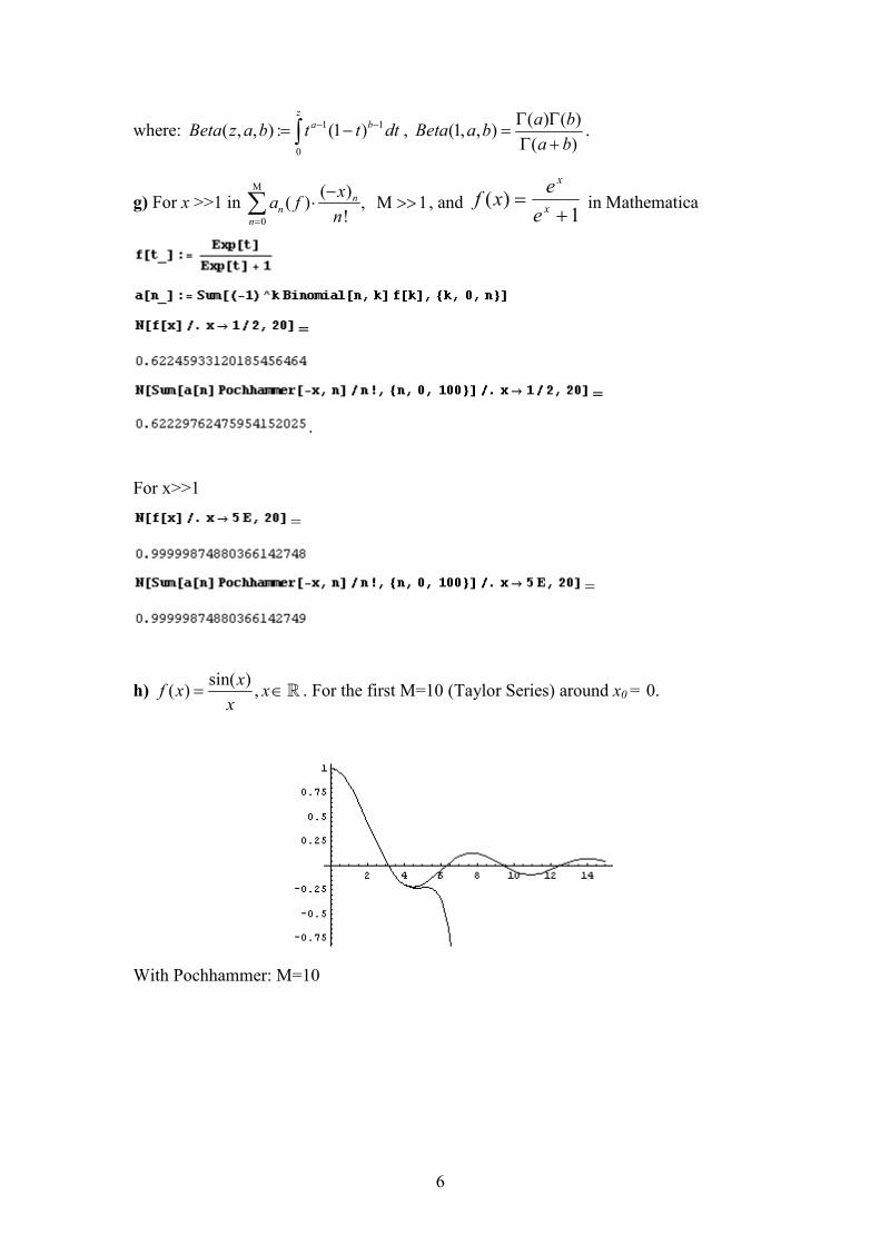
g) For x >>1 in 0
( )( ) , Μ 1
!
nn
n
xa f
n
Μ
=
−⋅ >>∑ , and
1)(
+=
x
x
e
exf in Mathematica
=
=
.
For x>>1
=
=
h) sin( )
( ) ,x
f x xx
= ∈ℝ . For the first M=10 (Taylor Series) around x0 = 0.
With Pochhammer: M=10

7
Proposition.
0 0 0
( )( 1) ( 1)( ) ( ) ( )
! ! !
k l
k
k k l
a ff k g k g k l
k k l
∞ ∞ ∞
= = =
− −= +∑ ∑ ∑
1) If 1
( )( )t
f tc
= and ( ) tg t a= , we get:
1/ 2 / 2 1 11
0
( , ,1)(2 ) ( )
!
c a n
c
n
F n ca e J a c a
n
∞−
−=
−⋅ ⋅Γ =∑ .
2) If ( ) , ( ) (1/ 2)t
tf t x g t −= = , then
1/ 2
0
( 1)cosh(2 ) (2)
!
n
n
n
xx I
nπ
∞
− +=
−= ∑ .
Let 0( ) ( / 4)f t J t= then ( )b
af t dt∫ for a=-e, b=π
1 1( )
1
0 0
( )( 1)
! 1
m mM nn mn
n
n m
a f b aS
n m
+ +
= =
−−
+∑ ∑ για Μ = 100:
Let f be analytic in ℝ , then if
0
( ) ( 1) ( )n
k
n
k
na f f k
k=
= −
∑ ,
and

8
0
0 ( )n
n
a f∞
=
< < ∞∑ ,
then
0
( )( ) ( )
!
nn
n
xf x a f
n
∞
=
−= ⋅∑ ,
Where ( )
( ) ( 1)( 2) ... ( 1)( )
n
x nx x x x x n
x
Γ += = + + ⋅ ⋅ + −
Γ
A kind of Proof. (for the complete Proposition see [M,B] )
( )
0
(0)( )
!
nn
n
ff x x
n
∞
=
=∑ .
( )
2
0 0
(0)( ) ( 1)...( 1)
!
n nm
n
n m
ff x S x x x m
n
∞
= =
= − − +
∑ ∑ .
But
∑=
−
−=
m
k
nkmm
n kk
m
mS
0
2 )1(!
1 (1)
∑ ∑ ∑∞
= = =
−
+−−
−=
0 0 0
)(
)1)...(1()1(!
1
!
)0()(
n
n
m
m
k
nkmn
mxxxkk
m
mn
fxf
=∑ ∑ ∑∞
= = =
−
−
0 0 0
)(
)()1(!
1
!
)0(
n
n
m
m
m
k
nmn
xkk
m
mn
f
=∑ ∑ ∑∞
=
∞
= =
−
−
0 0 0
)(
)()1(!
1
!
)0(
n m
m
m
k
nmn
xkk
m
mn
f
=∑ ∑∞
= = −−
−0 0
)(!)!(
)1()(
m
m
k
m
m kfkkm
x .
Corollary
f, g analytic:
0 0 0
( )( 1) ( 1)( ) ( ) ( )
! ! !
k l
k
k k l
a ff k g k g k l
k k l
∞ ∞ ∞
= = =
− −= +∑ ∑ ∑ ,
Proof.
0
( )( ) ( )
!
mm
m
a ff x x
m
∞
=
= ⋅ −∑

9
0
( ) ( )( )
! ( )
m
m
a f x mf x
m x
∞
=
Γ − += ⋅
Γ −∑
Hence
0
( )( ) ( ) ( )
!
m
m
a ff x x x m
m
∞
=
Γ − = ⋅Γ − +∑
Hence
0
( )( ) ( ) ( ).
!
m
m
a ff ix ix ix m
m
∞
=
− Γ = ⋅Γ +∑
0
( )( ) ( ) ( ) ( ) ( )
!
s
s
a fg xi f xi xi xi s g xi
s
∞
=
− − Γ = ⋅Γ + −∑ . (α)
Integrating we get the result
(remember that)
( )
10
(0)( )( )( ) 2 lim ( ( ))
!
mm
rm
f t M x it dt f i x m rm
π−
∞ ∞
→ =−∞
ΨΨ + = ⋅ +∑∫
Let f analytic Taylor in ℝ , then , , a b a b∈ <ℝ :
( ) =
b
a
f t dt∫1 1
( )
1
0 0
( )( 1)
! 1
m mnn mn
n
n m
a f b aS
n m
+ +∞
= =
−−
+∑ ∑ .
Proof.
Let ,a b∈ℝ , a b< then:
( )
b
a
f t dt =∫0
( )( )
!
b
nn
n a
a fx dx
n
∞
=
−∑ ∫ . (β)
( )
1
m
nS Stirling first kind then:
( ) ( 1) ( 1)...( 1)n
nx x x x n− = − − − + = ( )
1
0
( 1)n
n m n
n
m
S x=
− ∑ . (γ)
From (β),(γ) we get the proof.

Some New Results on Prime Sums
Nikos BagisDepartment of Informatics
Aristotle University of Thessaloniki54124 Thessaloniki, Greece
Abstract
In this work we cosider sums of primes. We set as a basea generalization of Euler’s prime number theorem and we usethe values of Riemann Zeta function for the approximation.We also give the truncation error of these approximations
keywords Number Theory; Prime Sums; Elliptic Theta Functions;Euler-Totient Constant
1

1 Finite Sums and Products
Theorem 1Let f be analytic in A ⊇ (−1, 1] with f(0) = 0. Let also an is an arbitrarysequence such that |an| < 1, for n = 1, 2, 3, .... Then we have
∑k≤x
f(ak) = −∞∑n=1
log
∏k≤x
(1− ank )
1n
∑d|n
f (d)(0)Γ(d)
µ(n/d) (1)
Where x is a positive integer and µ is the Moebius Mu function defined by
µ(n) =
1, if n = 1(−1)r, if k = the product of r distinct primes
0, othewize
(2)
Proof.
−∞∑n=1
cn log
∏k≤x
(1− ank )
= −∞∑n=1
cnn
x∑k=1
log(1−ank ) =∞∑n=1
cnn
x∑k=1
∞∑m=1
1mamnk =
=x∑k=1
∞∑n=1
∞∑m=1
cnnm
amnk =x∑k=1
∞∑r=1
1rark∑d|r
cd (3)
Let now1r
∑d|r
cd =f (r)(0)r!
From the Moebius Inversion Theorem (see Theorem (ii)) of this article, or formore details one can see [Ap] chapter 2. we get that
cr =∑d|r
f (d)(0)Γ(d)
µ(r/d)
Hence equation (3) becomes
−∞∑n=1
log
∏k≤x
(1− ank )
1n
∑d|n
f (d)(0)Γ(d)
µ(n/d) =x∑k=1
∞∑r=1
f (r)(0)r!
(ak)r =x∑k=1
f(ak)
2

2 The extension of Euler’s Theorem
Theorem 2.If f is analytic in A ⊇ (−1, 1] and f(0) = 0, then we have
A(s) :=∑
p−primef
(1ps
)=∞∑n=1
log(ζ(sn))n
∑d|n
f (d)(0)Γ(d)
µ(n/d) (4)
Where the first sum is over all prime, and ζ is the Riemann’s Zeta functionζ(s) =
∑∞n=1 1/ns, s > 1.
Proof.Set an = 1/psn, where pn is the n-th prime, s > 1 and x = ∞. Then usingEuler’s Theorem
1/ζ(s) =∏
p−prime
(1− 1
ps
), s > 1 the result follows easily from Theorem 1.
Proposition 1.The Truncation Error of (3) is
E(f,M, s) :=
∣∣∣∣∣∣∞∑
n=M+1
log(ζ(ns))n
∑d|n
f (d)(0)Γ(d)
µ(n/d)
∣∣∣∣∣∣ (5)
then
E(f,M, s) ≤ 2s+1(2s + 1)(s+ 1)M2
π(2s − 1)3(sM + s− 1)2sM
∫ 2π
0
∣∣f(eit)∣∣ dt (6)
Proof.Let
E =
∣∣∣∣∣∣∞∑
n=M+1
log(ζ(ns))n
∑d|n
f (d)(0)Γ(d)
µ(n/d)
∣∣∣∣∣∣First from the Poisson formula we have
f (k)(0)k!
=1
2π
∫ 2π
0
f(eit)e−itkdt
thus ∣∣∣∣fk(0)Γ(k)
∣∣∣∣ ≤ k
2π
∫ 2π
0
∣∣f(eit)∣∣ dt
3

∣∣∣∣∣∣∑d|n
f (d)(0)Γ(d)
µ(n/d)
∣∣∣∣∣∣ ≤n∑k=1
∣∣∣∣f (k)(0)Γ(k)
∣∣∣∣ ≤ 12π
∫ 2π
0
∣∣f(eit)∣∣ dt n∑
k=1
k
and the error becomes
E ≤ 14π
∫ 2π
0
∣∣f(eit)∣∣ dt ∣∣∣∣∣
∞∑n=M+1
(n+ 1) log(ζ(sn))
∣∣∣∣∣ ≤from the inequality log(x) ≤ x− 1 we arive at
E ≤ 14π
∫ 2π
0
∣∣f(eit)∣∣ dt ∞∑
n=M+1
(n+ 1)(
12sn
+1
3sn+
14sn
+ ...
)(7)
We will try to estimate the series
A(x) :=12x
+13x
+14x
+ ...,
x = sn
A(x) =12x
+13x
+14x
+ ... ≤ 12x
+∫ ∞
2
1txdt =
=1
2sn+
2(sn− 1)2sn
=(sn+ 1)
2sn(sn− 1)
Thus we can write
E ≤ 14π
∫ 2π
0
∣∣f(eit)∣∣ dt ∞∑
n=M+1
(n+ 1)sn+ 1
2sn(sn− 1)
observe that n+ 1 ≤ 2n, 1/(sn− 1) ≤ 1/(s(M + 1)− 1), thus
E ≤ 24π(sM + s− 1)
∫ 2π
0
∣∣f(eit)∣∣ dt ∞∑
n=M+1
n(sn+ 1)2sn
≤
E ≤ s+ 12π(sM + s− 1)
∫ 2π
0
∣∣f(eit)∣∣ dt ∞∑
n=M+1
n2
2sn=
=s+ 1
2π(sM + s− 1)2sM
∫ 2π
0
∣∣f(eit)∣∣ dt ∞∑
n=1
(n+M)2
2sn
=s+ 1
2π(sM + s− 1)2sM
∫ 2π
0
∣∣f(eit)∣∣ dt ∞∑
n=1
n2 + 2nM +M2
2sn≤
≤ s+ 12π(sM + s− 1)2sM
∫ 2π
0
∣∣f(eit)∣∣ dt ∞∑
n=1
4n2M2
2sn≤
4

≤ 2s+1(2s + 1)(s+ 1)M2
π(2s − 1)3(sM + s− 1)2sM
∫ 2π
0
∣∣f(eit)∣∣ dt
and we get the estimate
General observations and motivationsi) Let φ(q) =
∑∞k=−∞ qk
2, |q| < 1, then
∑p−prime
log(φ
(1ps
))=∞∑n=1
log(ζ(sn))n
∑d|n
f (d)(0)Γ(d)
µ(n/d) (8)
where f(x) = log(φ(x)). We try to calculate
X(n) :=1n
∑d|n
f (d)(0)Γ(d)
µ(n/d)
From ([Be3], pg. 36) we have the following representation of φ
φ(q) =(−q,−q)∞(q,−q)∞
where (a; q)∞ :=∏∞n=0(1− aqn).
Hence
log(φ(q)) =∞∑n=1
log(1− (−q)n)−∞∑n=1
log(1 + (−q)n) =
=∞∑n=1
∞∑m=1
(−1)m
m(−q)nm −
∞∑n=1
∞∑m=1
1m
(−q)nm =
=∞∑n=1
(−1)n
∑d|n
(−1)d − 1d
qn
Hence
X(n) =1n
∑d|n
(−1)d
∑δ|d
((−1)d/δ − 1)δ
µ(n/d)
which one can see numerically that
X2(n) =
2, n ≡ 1mod4−3, n ≡ 2mod42, n ≡ 3mod4−1, n ≡ 0mod4
(9)
We prove that X is mod4 periodic:
5

It is known ([Be3], pg.36) that holds∞∑
k=−∞
qk2
=∞∏n=0
(1 + q2n+1)(1− q2n+2)(1− q2n+1)(1 + q2n+2)
=∞∏n=1
(1 + q2n−1)(1− q2n)(1− q2n−1)(1 + q2n)
Hence from the relations ∏p−prime
(1− 1
ps
)=
1ζ(s)
, s > 1
∏p−prime
(1 +
1ps
)=
ζ(s)ζ(2s)
, s > 1
∏p−prime
φ
(1ps
)=
=∞∏n=1
∏p−prime
(1 +
1p(2n−1)s
)(1− 1
p2ns
)(1− 1
p(2n−1)s
)−1(1 +
1p2ns
)−1
=
=∞∏n=1
ζ2((2n− 1)s)ζ2(4ns)ζ(2(2n− 1)s)ζ2(2ns)
= ... =∞∏n=1
ζ2(ns)ζ2(4ns)ζ5(2ns)
Having in mind the above we can write∏p−prime
φ
(1ps
)=∞∏n=1
ζ2(ns)ζ2(4ns)ζ5(2ns)
=∞∏n=1
ζ(sn)X2(n) (10)
where s > 1For to prove the periodicity of X2 we go backwards. The only thing that leftis the uniqueness of the expansion but this follows from the continuity of ζ(s),when s > 1 (see [Kor] pg.15).Note that we work with
∑∞k=−∞ qk
2and not with
∑∞k=−∞ qk
2.
ii) Also one can seeSet ψ(q) =
∑∞k=−∞ qk(k+1)/2, |q| < 1 then
1n
∑d|n
µ(n/d)Γ(d)
∂d
∂xd(log(ψ(x)))x=0 = −(−1)n (11)
We will show that if θ(q) is a theta function, obeying some certain conditionsthen X(n) is a periodic sequence having values only 0 and 1.From [An] pg. 178 we have
Theorem(i).(The Jacobi triple product identity)There holds the following factorization formula
∞∑n=−∞
(−1)nqkn2+hn =
∞∏n=0
(1− q2kn+2k)(1− q2kn+k−h)(1− q2kn+k+h) (12)
6

From [Ap] we have
Theorem(ii).(The Moebius inversion formula)If f , g are arithmetic functions then we have∑
d|n
f(d)µ(n/d) = g(n)⇔ f(n) =∑d|n
g(d) (13)
Theorem 3. If we set θ(q) =∑∞n=−∞(−1)nqkn
2+hn with k, h ∈ N, k > h > 0then holds the following relation
1n
∑d|n
µ(n/d)Γ(d)
(∂d
∂xdlog(ψ(x))
)x=0
= Xk,h(n) (14)
where
Xk,h(n) =
1, n ≡ 0modp
1, n ≡ k + hmodp1, n ≡ k − hmodp
0, else
(15)
Proof.It is
∞∑n=−∞
(−1)nqkn2+hn =
∞∏n=0
(1− q2kn+2k)(1− q2kn+k−h)(1− q2kn+k+h) (16)
Observe that
θ(q) =∞∑
n=−∞(−1)nqkn
2+hn =∞∏n=1
(1− qn)Xk,h(n) (17)
we can write
log(θ(q)) =∞∑n=1
Xk,h(n) log(1− qn) = −∞∑n=1
Xk,h(n)∞∑m=1
1mqmn =
= −∞∑n=1
∞∑m=1
1mXk,h(n)qmn
or
log(θ(q)) = −∞∑n=1
∑d|n
Xk,h(d)n/d
qn = −∞∑n=1
∑d|n
Xk,h(d)d
qn
n
Thus1n!
(∂n log(θ(q))
∂qn
)q=0
= − 1n
∑d|n
Xk,h(d)d
7

An equivalent form using Theorem(ii) is
− 1n
∑d|n
µ(n/d)Γ(d)
(∂d log(θ(q))
∂qd
)q=0
= Xk,h(n) (18)
3 The Euler Totient constant
When n is a positive integer, Euler’s Totient function φ(n), is defined to be thenumber of positive integers not greater than n and relatively prime to n. Inter-esting constants emerge if we consider the sum of reciplocals of φ(n). Landauproved that
N∑n=1
1φ(n)
= a log(N) + b+O
(log(N)N
)where
a =∞∑k=1
µ(k)2
kφ(k)=ζ(2)ζ(3)ζ(6)
=315ζ(3)
2π4= 1.9435964368 . . .
and
b =315ζ(3)
2π4−∞∑k=1
µ(k)2 log(k)kφ(k)
= −0.06057 . . .
In the above formulas, ζ(x) is the Riemannn’s zeta function and ζ(3) is Apery’sconstant.An alternative expression for the constant b is
b =315ζ(3)
2π4
γ − ∑p−prime
log(p)p2 − p+ 1
= −0.06057 . . .
We will show how to estimate the value of prime series, such as∑p−prime
log(p)p2 − p+ 1
(19)
For this we set
f1(x) =1√3
arctan(
2x− 1√3
)+
12
log(1− x+ x2) (20)
then
b =3152π4
ζ(3)
γ +∞∑n=2
ζ′(n)
ζ(n)
∑d|n
f(d)1 (0)Γ(d)
µ(n/d)
We can calculate (19), setting f1 in (4) and differentiating with respect to s.Then
lims→1+
∑p
f ′1
(1ps
)log(p)ps
=∑p
log(p)p2 − p+ 1
8

Proposition 3.If we set
E1 = E(f1,M) :=
∣∣∣∣∣∣∞∑
n=M+1
ζ′(n)
ζ(n)
∑d|n
f(d)1 (0)Γ(d)
µ(n/d)
∣∣∣∣∣∣when M >> 1 then
E(f1,M) ≤ (2M + 4)ζ′(M + 1)
where ζ′
is the derivative of the Riemann’s Zeta function.
Proof.If a(k) = f
′
1(0)k/k!, then f(0) = 0 and
a(n) =
0, n ≡ 1mod61, n ≡ 2mod61, n ≡ 3mod60, n ≡ 4mod6−1, n ≡ 5mod6−1, n ≡ 0mod6
(21)
Note. The values of a(k) follow fromh(x) = d
dx
(1√3
arctan(
2x−1x
)+ 1/2 log(1− x+ x2)
)= x/(x2 − x+ 1),
h(1/x) = h(x) andh(x) = x/(x− p1)(x− p2) =
(∑∞k=0(xp1)k −
∑∞k=0(xp2)k
)/(p1 − p2) = . . .
p1, p2 are the roots of x2 − x+ 1 = 0.Also one can see that a(k) = 2√
3sin((k − 1)π/3), for k = 1, 2, 3, . . .
Hence ∣∣∣∣∣∣∑d|n
f(d)1 (0)µ(n/d)
Γ(d)
∣∣∣∣∣∣ <∑d|n
|µ(d)| ≤ d(n) ≤ n
where d(n) =∑d|n 1. Thus
E(f1,M) ≤∞∑
n=M+1
∣∣∣∣∣ζ′(n)
ζ(n)
∣∣∣∣∣ d(n) ≤∞∑
n=M+1
|ζ ′(n)|n =∞∑
n=M+1
∞∑k=2
log(k)kn
n =
∞∑k=2
log(k)k
∞∑n=M
n+ 1kn
=∞∑k=2
log(k)kM
(k −M + kM
(k − 1)2
)≤
∞∑k=2
log(k)kM
(4k
+2Mk
)= (2M + 4)ζ
′(M + 1)
9

4 Finite Sums
Theorem 4.Let x be an integer greater than 1, s is real, s > 1 and g analytic function inA ⊇ (−1, 1], such that g(a)(0)/a! are bounded above. Then∑
n≤x
µ(n)n
∞∑k=1
∞∑l=1
1lg
(1psnlk
)=∞∑k=1
g
(1psk
)+O
(xg
(1
2s(x+1)
))(22)
when x >> 1
Proof.∞∑k=1
1psk
= −∞∑n=1
µ(n)n
log
( ∞∏k=1
(1− 1
psnk
))=
= −M∑n=1
µ(n)n
log
( ∞∏k=1
(1− 1
psnk
))−
∞∑n=M+1
µ(n)n
log
( ∞∏k=1
(1− 1
psnk
))=
= −∞∑n=1
µ(n)n
∞∑n=1
log(
1− 1psnk
)+
∞∑n=M+1
µ(n)n
log(ζ(sn)) =
=M∑n=1
µ(n)n
∞∑k=1
∞∑l=1
1psnlk
+∞∑
n=M+1
µ(n)n
log(ζ(sn))
Thus we get∞∑k=1
1psk−
M∑n=1
µ(n)n
∞∑k=1
∞∑l=1
1lpsnlk
=∞∑
n=M+1
µ(n)n
log(ζ(sn))
Hence ∣∣∣∣∣∞∑k=1
1psk−
M∑n=1
µ(n)n
∞∑k=1
∞∑l=1
1lpsnlk
∣∣∣∣∣ =∣∣∣∣∣∞∑
n=M+1
µ(n)n
log(ζ(sn))
∣∣∣∣∣ ≤C2s(2s + 1)(s+ 1)M2
(2s − 1)3(sM + s− 1)2sM≤
CM
2s(M+1)
Let now g(a)(0)/a!, a = 1, 2, 3, . . . are bounded above. We have
g(a)(0)a!
( ∞∑k=1
1psak−
M∑n=1
µ(n)n
∞∑k=1
∞∑l=1
1lpsnlak
)= O
(M
2sa(M+1)
g(a)(0)a!
)(23)
We sum the above estimation with respect to a. Since g(a)(0)/a! are boundedabove we get the result.
10

5 Asymptotic Sums of Primes
In what follows in this section we need to prove and use the following
Lemma.
log
∏p≤x
(1− 1
ps
)−1 = log(ζ(s)) +O
(x
xs log(x)
)(24)
and ∑p≤x
log(p)ps − 1
= −ζ′(s)
ζ(s)+O
(1
xs−1
)(25)
when x >> 1, s > 1
Proof.a)First we begin with
−∑
p−primelog(
1− 1ps
)= log(ζ(s))
or
−∑p≤x
log(
1− 1ps
)− log(ζ(s)) =
∑p>x
log(
1− 1ps
)But ∑
p>x
log(
1− 1ps
)= O
∑p≥x
1ps
= O
∞∑n=π(x)
1psn
=
= O
∞∑n=π(x)
1(n log(n))s
= O
(x
xs log(x)
)Where we have usedC1n log(n) < pn < C2n log(n), A1n/ log(n) < π(x) < A2n/ log(n),when n >> 1. For some costants A1, A2, C1, C2.b) From [Be1] pg. 129 we have
1ζ(s)
∞∑k=1
log(k)ks
=∑
p−prime
log(p)ps − 1
=∑p≤x
log(p)ps − 1
+∑p>x
log(p)ps − 1
(26)
We only have to estimate∑p>x
log(p)ps−1 , for large x.
∑p>x
log(p)ps − 1
= O
(∑p>x
p
ps
)= O
∑n=π(x)
pnpsn
= O
∑n=π(x)
1(n log(n))s−1
=
11

= O
(1
xs−1
)We begin with
Theorem 5.Let f be analytic in (−1, 1], f(0) = 0 and cn(f) :=
∑d|n
f(d)(0)Γ(d) µ(n/d). If
cn(f)/n is bounded above then∑p≤x
f
(1ps
)= A(s) +O
(1
xs−1 log(x)f
′(
1xs
))(27)
Where s > 1 and x >> 1.
Proof. From
log
∏p≤x
(1− 1
ps
)−1 = log(ζ(s)) +O
(1
xs−1 log(x)
)and from Theorem 1 we have
∑p≤x
f
(1ps
)= −
∞∑n=1
log
∏p≤x
(1− 1
psn
) cn(f)n
=
=∞∑n=1
cn(f)n
log(ζ(sn) +O
(x
xsn log(x)
))=
=∑p
f
(1ps
)+∞∑n=1
O
(x
xsn log(x)
)cn(f)n
Hence ∣∣∣∣∣∣∑p≥x
f
(1ps
)∣∣∣∣∣∣ =∞∑n=1
O
(x
xsn log(x)
)cn(f)n
=
= O
(x
log(x)
∞∑n=1
cn(f)es log(x)n − 1
)= O
x
log(x)
∞∑n=1
∑d|n
cd(f)
e−s log(x)n
=
= O
(x
log(x)
∞∑n=1
f (n)(0)Γ(n)
e−s log(x)n
)= O
(x
xs log(x)f
′(
1xs
))Where we have used i)
∞∑n=1
Aneny − 1
=∞∑n=1
∑d|n
Ad
e−ny
12

and ii)An =
∑d|n
cd(f)⇔ cn(f) =∑d|n
Adµ(n/d)
⇔∑d|n
f(d)(0)Γ(d)
µ(n/d) =∑d|n
Adµ(n/d)
or
An =f (n)(0)Γ(n)
Corollary 1.Let f be analytic in A ⊇ (−1, 1], f(0) = 0 and cn(f)/n is bounded above then∣∣∣∣∣∑
p
f
(1ps
)∣∣∣∣∣ < +∞
when s > 1.
Corollary 2.Let f be analytic in A ⊇ (−1, 1], f(0) = 0 and cn(f)/n is bounded above then∑
p≤x
f
(1ps
)= f(0)π(x) +A(s) +O
(x
xs log(x)f ′(
1xs
))
where s > 1 and π(x) =∑p≤x 1.
In the same way as in Theorem 5 using the asymptotic formula (25) we get
Theorem 6.Let f be analytic in A ⊇ (−1, 1], f(0) = 0 and cn(f)/n is bounded above then∑
p≤x
f′(
1ps
)log(p)ps
= −A′(s) +O
(1
xs−1f
′(
1xs
))when s > 1 and x >> 1.
References
[1]:G.E.Andrews, ’Number Theory’. Dover Publications, New York
13

[2]:T.Apostol, ’Introduction to Analytic Number Theory’. Springer Verlang,New York
[3]:B.C.Berndt, Ramanujan‘s Notebooks Part I. Springer Verlang, New York(1985)
[4]:B.C.Berndt, ’Ramanujan‘s Notebooks Part III’. Springer Verlang, NewYork (1991)
[5]:Konrad Knopp, ’Theory and Application of Infinite Series’. Dover Pub-lications, Inc. New York. 1990
[6]:T.W.Korner.’Fourier Analysis’. Cambridge University Press, Cambridge,New York, New Rochelle, Melbourne, Sydney.
[7]:William J. LeVeque. ’Fundamentals of Number Theory’. Dover Publica-tions, Inc. New. York 1996.
14

A Pochhammer type sampling reconstruction of analytic functions
A. MelasUniversity of Athens Department of Mathematics Panepistimiopolis Athens15784 [email protected]
N. BagisAristotle University of Thessaloniki Department of Informatics [email protected]
Abstract
We give a characterization of the functions f analytic on the halfplaneRe(z) > σ that can be expressed in the form f(z) =
∑∞n=0 βn
(−z)nn!
for some βn ∈ C. It will follow that the βn depend on the valuesof f on the integers so this gives a sampling reconstruction of thesefunctions. Several examples of this representation are given.
1

1 Introduction and The Main Theorem
Every polynomial can be written as a product of linear factors. Entire functionsbehave in much the same way: if f(z) is entire then f can reconstructed by itszeros (Under some certain conditions).Also a polynomial can always be recovered by the values of the polynomial inthe set of integers. Can we recover entire functions under some conditions fromtheir values on the set of integers? One known example of this idea, is theShannon’s Sampling Theorem for band limited functions (see [2]). Many resultshave been published and come to light in this area.Here we give a new not band limited type reconstruction.We will study here the class U of functions f that are analytic in some half-planeof the form{z ∈ C : Re(z) > σ}, σ > 0 and such that there exist βn ∈ C, n = 1, 2, . . . with
f(z) =∞∑n=0
βn(−z)nn!
(1.1)
uniformly on compact subsets of a possibly smaller half plane Re(z) > σ′ ≥ σ.Here (w)n = w(w+1) . . . (w+n−1) is the Pochhammer symbol. Our main resultis a characterization of such functions. To describe it we define the followingset:
A ={γ ∈ C : |Im(γ)| < π
2, |1− eγ | ≤ 1
}=
={α+ iβ ∈ C : |β| < π
2, α ≤ log(2 cos(β))
}Then we will show the following:Theorem 1. (a) The following are equivalent(i) f belongs to U .(ii)There exist σ1 > 0, a polynomial p(z) and a finite complex Borel measure µsupported on A such that:
f(z) = p(z)∫A
e(z−σ)γdµ(γ) (1.2)
(iii) There exist σ2 > 0 and constants N,C > 0 such that:
|f(z + σ2)| ≤ C(2x)x∣∣z−z∣∣ (1 + |z|N ) (1.3)
whenever x = Re(z) > 0.(b) If f belongs to U and (1.1) holds on Re(z) ≥ σ′ then we can define (orredefine) the values the values f(k) for k integer with 0 ≤ k ≤ σ′ in such a waythat:
βn =n∑k=0
(−1)k (nk ) f(k) (1.4)
for all n ≥ 0.The other values of f(k), k > σ′ are those of f . Actually the above theorem
2
provides a sampling reconstruction of f by it values on the integers. Note thatthe values f(k) for 0 ≤ k ≤ σ′ may be different from the values of the functionf , or its analytic continuation has at those points as we will show by examples.Also the equivalence (ii) and (iii) is more or less well known using analytic func-tions on unbounded supports but we will give here a proof here for completeness.The main fact in this paper is of course the equivalence of (i) with (ii) or (iii).
2 The series representation
First we will show the following:Proposition 1.Suppose z0 is not a nonnegative integer and that the series
∑∞n=0 βn
(−z)nn! has
bounded partial sums. Then the series
f(z) =∞∑n=0
βn(−z)nn!
(2.1)
converges uniformly on compact subsets of {z ∈ C : Re(z) > Re(z0)} and definesan analytic function there. Moreover one can define the values f(k) for integersk with 0 ≤ k ≤ Re(z0) (if any) such that
βn =n∑k=0
(−1)k (nk ) f(k) (2.2)
for all n ≥ 0.Proof.Let K ⊆ {z ∈ C : Re(z) > Re(z0)} be compact and let Mk, εk be such thatεk + Re(z0) ≤ Re(z) ≤ Mk whenever z ∈ K. Consider now a z ∈ K. Then forn > Mk + 1 we have:
βn(−z)nn!
= βn(−z0)nn!
Γ(−z0)Γ(−z)
Γ(n− z)Γ(n− z0)
so since 1Γ(−z) is bounded on K it suffices by Abel’s test to prove that∑
n>Mk+1 |bn(z)− bn+1(z)| converges uniformly on K where bn = Γ(n−z)Γ(n−z0) . But
since Re(n− z), Re(n− z0) > 1 Stirling’s formula implies
|bn(z)| ≤ c1∣∣∣∣ e−n+z(n− z)n−z−1/2
e−n+z0(n− z0)n−z0−1/2
∣∣∣∣ ≤ Ckn−(Re(z)−Re(z0)) ≤ Ckn−εk
where Ck > 0 is a constant that depends only on K.Hence for any n > Mk + 1:
|bn(z)− bn+1(z)| = |bn(z)|∣∣∣∣1− n− z
n− z0
∣∣∣∣ ≤ Ck |z − z0||n− z0|
n−εk ≤ C ′kn1+εk
3

and this completes the proof of the uniform convergence.Next define f(k) for 0 ≤ k ≤ Re(z0) so that (2.2) holds that is f(0) = β0, f(1) =f(0) − β0, . . . , (−1)kf(k) = βk −
∑k−1m=0(−1)m (nk ) f(m), for k ≤ Re(z0). Then
we will show that (2.2) holds for all n.Indeed supposing it holds for 0, 1, 2, . . . , n− 1 where n > Re(z0), (2.1) gives
f(n) =n∑k=0
βk(−n)kk!
=n−1∑k=0
βk(−1)k (nk ) + (−1)nβn =
n−1∑k=0
k∑m=0
(−1)m(km
)f(m)(−1)k (nk ) + (−1)nβn
hence
βn = (−1)nf(n)−n−1∑m=0
[n−1∑k=m
(−1)m+k+n (nk )(km
)]f(m) =
(−1)nf(n)−n−1∑m=0
(−1)m (nm) f(m)n−1∑k=m
(−1)n+k(n−mk−m
)and this gives (2.2) since
n−1∑k=m
(−1)n+k(n−mk−m
)= −1
To proceed further we need the following:Lemma 1.Let z ∈ C be such that Re(z) > 0 and for a ∈ C with |1− a| ≤ 1 define:
SN (a) =N∑n=0
(1− a)n(−z)nn!
Then SN → az as N →∞ and there exists a constant Cz > 0 independent of asuch that:
|az − SN (a)| ≤ Czfor all such a.Proof.Considering the function F (w) = wz = exp(z log(w)) analytic onC− (−∞, 0] (where log is real and positive on (1,+∞) ) we have
F (w)−N∑n=0
(w − 1)nF (n)(1)n!
=(w − 1)N+1
2πi
∫γR
F (ζ)dζ(ζ − 1)N+1(ζ − w)
where γR is the line segment from 0 to −R followed by the circle centered at 0and of radius R followed by the line segment from −R to 0 on the next sheet
4

of the Riemann surface of log(w) and then taking R→∞ we get if N > Re(z)that
|az − SN (a)| =∣∣∣∣ (1− a)N+1
2πi(eiπz − e−iπz
) ∫ ∞0
zz
(t+ 1)N+1(t+ a)
∣∣∣∣ ≤|sin(πz)|
π
∫ ∞0
tRe(z)−1
(t+ 1)N+1dt
since Re(z) > 0 and |t+ a| > t whenever t > 0 and |1− a| ≤ 1.This proves the Lemma.The following will be needed here and in the examples.Proposition 2.Let A1, A2 ⊆ A be such that A1 +A2 ⊆ A. If s1, s2 ∈ R and
f1(z) =∫A
e(z−s1)γdµ1(γ), f2(z) =∫A
e(z−s2)γdµ2(γ) (2.3)
on Re(z) > s1 and Re(z) > s2 respectively where µ1, µ2 are finite complex Borelmeasures on A1, A2 respectively then there exists a Borel measure µ on A suchthat:
f1(z)f2(z) =∫A
e(z−s)γdµ(γ) (2.4)
on x > s = max(s1, s2).Proof.Suppose that s1 > s2. Then by Fubini‘s theorem we can takeµ = µ1∗(e(s1−s2)µ2) which is supported on A1+A2 ⊆ A and note that wheneverRe(z) > s:∫
A1
∫A2
∣∣∣e(z−s)(γ1+γ2)∣∣∣ ∣∣∣e(s1−s2)γ
∣∣∣ d |µ1| (γ)d |µ2| (γ) < +∞
Now we can prove the implication (i)⇒ (ii) in Theorem 1.Proposition 3.Let the function f be given by (2.1) where the series converges uniformly oncompact subsets of Re(z) > σ. Choose an integer s ≥ 0 such that s > 3/2 + σ.Then(i) There exist a polynomial p1(z) of degree ≤ s−1 and a function h ∈ L2(0, 2π)such that:
f(z) = p1(z) + z(z − 1) . . . (z − s+ 1)∫ 2π
0
(1− eiθ)z−sh(θ)dθ
for every z with Re(z) > s.(ii) There exists a polynomial p(z) of degree s and a finite Borel measure µ onA such that:
f(z) = p(z)∫γ
e(z−s)γdµ(γ)
5

whenever Re(z) > s.Proof.(i) By (2.1) we can write:
f(z) = p1(z) +∞∑n=s
βn(−z) . . . (−z + s− 1)(−z + s) . . . (−z + n− 1)
n(n− 1) . . . (n− s+ 1)(n− s)!=
p1(z) + (−1)sz(z − 1) . . . (z − s+ 1)∞∑m=0
βm+s
(m+ 1) . . . (m+ s)(−z + s)m
m!
where deg p1(z) ≤ s− 1.Choose σ > σ with s > 3/2+σ that is not a nonnegative integer. Then Stiring’sformula gives for all large n: ∣∣∣∣ (−σ)n
n!
∣∣∣∣ ≥ cn−1−σ
Since the series defining f(σ) converges(βn
(−σ)nn!
)n≥0
must be bounded hence
|βn| ≤ Cn1+σ for all n and some constant C > 0. This implies that:
∞∑m=0
∣∣∣∣ βm+s
(m+ 1) . . . (m+ s)
∣∣∣∣2 ≤ Cs ∞∑m=0
m2(1+σ−S) < +∞
therefore there exists h ∈ L2(0, 2π) such that:
βm+s
(m+ 1) . . . (m+ s)=∫ 2π
0
eimθh(θ)dθ
for all m ≥ 0.But for Re(z) > s, Lemma 1 implies that
∑Nm=0 e
imθ (−z+s)mm! converges to
(1− eiθ)z−s boudedly on (0, 2π) and hence by the dominated convergence the-orem we have:
∞∑m=0
βm+s
(m+ 1) . . . (m+ s)(−z + s)m
m!= limN→∞
∫ 2π
0
N∑m=0
eimθ(−z + s)m
m!h(θ)dθ
=∫ 2π
0
(1− eiθ)z−sh(θ)dθ
This proves (i).(ii) Since the mapping (0, 2π) 3 θ → log(1− eiθ) ∈ ∂A is continuous one to oneand onto (−1)sh(θ)dθ induces a finite complex Borel measure µ0 on ∂A ⊆ A.Hence (i) gives:
f(z) = p1(z) + z(z − 1) . . . (z − s+ 1)∫∂A
e(z−s)γdµ0(γ)
6

and since1
zk+1=
1k!
∫ ∞−∞
e−tztkdt
(Re(z) > 0) for any integer k ≥ 0, (ii) follows from Proposition 2, since(−∞, 0) + ∂A ⊆ A.
3 The equivalence (ii)⇔ (iii)
The implication (ii)⇔ (iii) in Theorem 1 is easy. Clearly from (1.2):
|f(z + σ1)| = C(1 + |z|N )∫A
eRe(zγ)d |µ| (γ)
where Re(z) > 0, N = deg p.Thus it suffices to prove that eRe(zγ) ≤ (2x)x |z−z| whenever x = Re(z) > 0and γ ∈ A. But setting z = x+ iy, γ = α + iβ where |β| < π/2, eα ≤ 2 cos(β),we get: eRe(zγ) ≤ (2 cos(β))xe−βy which is maximized on β ∈
(−π2 ,
π2
)when
tan(β) = −y/x giving:
eRe(zγ) ≤
(2x√x2 + y2
)xey arctan( yx ) = (2x)x
∣∣z−z∣∣To give a self contained proof of the implication (iii) ⇒ (ii) we first prove thefollowing:Lemma 2.Suppose f is analytic on Re(z) > 0 and satisfies
|f(z)Γ(z)| ≤ C(
2xe
)x 1|z|2
(3.1)
for some constant C, whenever x = Re(z) ≥ 1/3. Then given σ > 1/2 thereexists a finite complex measure µ on A such that:
f(z) =∫A
e(z−σ)γdµ(γ)
on Re(z) > σ.Proof.For x, t > 0 let
H(t, y) =1
2π
∫ ∞−∞
f(x+ it)Γ(x+ it)y−x−itdt (3.2)
By Cauchy’s Theorem and (3.1) we easily get that H is independent of x aslong as x ≥ 1/3 so we may write H(t, x) = H(t) for x ≥ 1/3 and t > 0.If t ≥ 1 we have:
2π |H(t)| = 2π∣∣∣H(t, t/2)
∣∣∣ ≤ C ∫ ∞−∞
t−1/3 dy
|1/3 + iy|2≤ C2t
−1/3
7
Hence et/2H(t)X(0,+∞)(t) is in L2(R) and therefore there exists g ∈ L2(R) suchthat:
H(t) =∫ ∞−∞
e−itξ−t/2g(ξ)dξ (3.3)
for t > 0 which actually means:
H(t) = limε→0+
∫ ∞−∞
e−t(1/2+iξ)e−ε|ξ|2g(ξ)dξ (3.4)
IfRe(z) > 1/2 the Mellin transform inversion formula together with the estimateH(t) ≤ C min
(e−t/2
z , t−1/3)
implies that:
f(z)Γ(z) =∫ ∞
0
tz−1H(t)dt =∫ ∞
0
tz−1 limε→0+
∫ ∞−∞
e−t(1/2+iξ)e−ε|ξ|2g(ξ)dξdt
(3.5)if we could take the limit outside the integral then we would get:
f(z)Γ(z) = limε→0+
∫ ∞0
tz−1
∫ ∞−∞
e−t(1/2+iξ)e−ε|ξ|2g(ξ)dξdt =
limε→0+
∫ ∞−∞
(∫ ∞0
tz−1e−t(1/2+iξ)dt
)eε|ξ|
2g(ξ)dξ =
= limε→0+
Γ(z)∫ ∞−∞
1(1/2 + iξ)z
e−ε|ξ|2g(ξ) dξ = Γ(z)
∫ ∞−∞
g(ξ)(1/2 + iξ)z
dξ
because Re(z) > 1/2 and g ∈ L2(R) imply that∫∞−∞
∣∣∣ g(ξ)(1/2+iξ)z
∣∣∣ dξ < +∞ so wecan apply the dominated convergence in the last step.Let σ > 1/2 be fixed.Since the mapping R 3 ξ → γ = log
(1
1/2+iξ
)∈ ∂A is one-to-one onto and
continuous (1/2 + iξ)−σg(ξ)dξ induces a finite measure µ on ∂A such that:
f(z) =∫∂A
e(z−σ)γdµ(γ)
on Re(z) > σHence to complete the proof of the Lemma it suffices to prove that the limit in(3.5) can be taken outside the integral. This can be done as follows:We have
|g(ξ)| = 2π∣∣∣et/2H(t)
∣∣∣ ≤ C min(
1t,
1t1/3
)≤ C(1 + |t|−1/3)
, for t > 0 and obviously (being 0) for t < 0. Hence:∣∣∣∣∫ ∞−∞
e−itξe−δ|ξ|2g(ξ)dξ
∣∣∣∣ =∣∣∣ e−δ|.|2 ∗ g(t)
∣∣∣ ≤ C
ε
∫ ∞−∞
e−−(t−u)2
4δ (1 + |u|−1/3)du ≤
8

C + 2C∫ ∞
0
e−s2 1
|1− λs|1/3ds
where λ =√ε|t| > 0.
Since∫∞
0
∣∣tz−1e−t/2t−1/3∣∣ dt < +∞ when Re(z) > 1/2 our claim will follow once
we proved that the function r(λ) =∫∞
0e−s
2 ds|1−λs|1/3 is (uniformly) bounded on
λ ∈ (0,+∞). But[∫ ∞2/λ
+∫ 1/(2λ)
0
]e−s
2 ds
|1− λs|1/3≤ 2
∫ ∞0
e−s2ds < +∞
∫ 2/λ
1/λ
e−s2 ds
|1− λs|1/3=
32λ
∫ 2/λ
1/λ
e−s2d(λs− 1)2/3 =
=3
2/λ
(e−4/λ2
+∫ 2/λ
1/λ
2se−s2(λs− 1)2/3ds
)≤ C
λ3e−1/λ2
and a similar inequality holds for∫ 1/λ
1/(2λ)e−s
2 ds|1−λs|1/3 . This completes the proof
since 1/λ3e−1/λ2is bounded on (0,+∞).
Now the implication (iii)⇒ (ii) can be proved as follows:Supposing f satisfies (1.3), in view of Stirling’s, formula, the function:
f(z) =1
(z + 1)N+3f(z + σ2)
satisfies (3.1) on x = Re(z) ≥ 1/3. Hence by Lemma 2 there exists µ0 suchthat:
f(z + σ2) = (z + 1)n+3
∫A
e(z−σ)γdµ0(γ)
where r > 2/3 > 1/3 when Re(z) > σ.Hence:
f(z) = (z − σ2 + 1)N+3
∫A
e(z−σ−σ2)γdµ(γ)
on Re(z) > σ + σ2 = σ1 hence f satisfies (1.2).This completes the proof of the equivalence (ii)⇔ (iii).
4 The implication (ii)⇒ (i)
Here we complete the proof of Theorem 1 by showing that if f satisfies (1.2)then it is in U.Clearly we may assume p(z) = zm for some integer m ≥ 0. First we have thefollowing:
9

Lemma 3.If γ ∈ C and 1 ≤ s ≤ n are integers then:
(1− eγ)n−s−1∑k=0
(nk ) (−1)kekγ = (−1)ss (ns ) eγs∫ 1
0
(1− teγ)n−s(1− t)s−1dt (4.1)
Proof.For γ ∈ R this follows from Taylor’s theorem hence by analytic continuation itholds for all γ ∈ C.Lemma 4.For each m, s integers there exist constants cm,r(s) for r = 0, 1, . . . ,m such that:(
∂
∂γ
)meγs(1− teγ)b =
m∑r=0
cm,r(s)b(b− 1) . . . (b− r + 1)(1− teγ)b−rtre(s+r)γ
(4.2)whenever γ, b ∈ C, t ∈ R are such that 1− teγ /∈ (−∞, 0].Moreover we have:
m∑r=0
(−1)rcm,r(s)w(w − 1) . . . (w − r + 1) = (w + s)m (4.3)
whenever w ∈ C.Proof.The equation (4.2) can be proved by an easy induction on m which actuallyimplies the recursion formula:
cm+1,r(s) = −cm,r+1(s) + (s+ r)cm,r(s) (4.4)
where cm,−1(s) = cm,m+1(s) = 0.To prove (4.3) we take t = −1 in (4.2) and R 3 γ → +∞ to get for any n > 0integer:
m∑r=0
(−1)rcm,r(s)n(n−1) . . . (n−r+1) = limγ→∞
(e−(n+s)γ
(∂
∂γ
)meγs(1 + eγ)n
)=
= limγ→∞
(e−(n+s)γ
∞∑k=0
(nk ) (k + s)me(k+s)γ
)= (n+ s)m
Hence as a polynomial equation (4.3) has infinitely many roots, thus it is anidentity.Now we have to prove the following:Proposition 4.Let µ be a finite Borel measure on A, σ ≥ 0 and p(z) a polynomial of degreem ≥ 0. Then for the function:
f(z) = p(z)∫A
e(z−σ)γdµ(γ) (4.5)
10
we have:(i) f is defined and analytic on the half-plane Re(z) > σ.(ii) If we give arbitrary values f(k) for k integers for 0 ≤ k ≤ σ and let
an(f) =n∑k=0
(−1)k (nk ) f(k) (4.5a)
for n = 0, 1, 2, . . ., then
f(z) =∞∑n=0
an(f)(−z)nn!
(4.6)
whenever Re(z) > [σ] + 1 +m.Proof.(i) Given z0 = x0 + iy0 ∈ C with x0 > σ let ε = 1/2(x0 − σ) > 0 and let M > 0be such that εM > π
2 (|y0|+ ε) and write:
A1 = A ∩ {Im(γ) ≥ −M} , A2 = A ∩ {Im(γ) < −M}
Then A1 is compact hence f1(z) = p(z)∫Ae(z−σ)γdµ(γ) is entire.
Now letg(z) =
∫A2
e(z−σ)γdµ(γ)
for z inside the square centered at z0 with side 2ε.If γ = α+iβ ∈ A2, z = x+iy is in this square then Re(z−σ)γ = (x−σ)α−yβ ≤−εM + (|y0|+ ε)π/2 thus∫A2
∣∣e(z−σ)∣∣ d |µ| (γ) ≤ |µ| (A2) < +∞. This in view of Morera’s theorem implies
that g and thus f is analytic.(ii) It is sufficient to assume that p(z) = zm. Let s = [σ] + 1 ≥ 1 and definef(k) = λk arbitrary for 0 ≤ k ≤ s (if any). Then an(f) =
∑nk=0 (nk ) (−1)kλk if
n < s and let for n ≥ s:
an(f) =∫A
n∑k=s
(nk ) (−1)ke(k−σ)γkmdµ(γ) +s−1∑k=0
(nk ) (−1)kλk =
∫A
{(∂
∂γ
)m [(1− eγ)m −
s−1∑k=0
(nk ) (−1)kekγ]}
e−σγdµ(γ) +s−1∑k=0
(nk ) (−1)kλk
This holds for all n since (nk ) = 0 for k > n. Hence by Lemma 3 we have:
an(f) =∫A
∫ 1
0
(∂
∂γ
)m(−1)ss (ns ) eγs(1−teγ)n−s(1−t)s−1dteσγdµ(γ)+
s−1∑k=0
(nk ) (−1)kλk
Now using Lemma 4 with b = n− s and summing for n = 0, 1, . . . , N we get ifz ∈ C is such that Re(z) > s+m
N∑n=0
an(f)(−z)nn!
11

= (−1)ss∫A
e(s−σ)γN∑n=0
m∑r=0
cn,r(s)(n− s) . . . (n− s− r + 1) (ns )(−z)nn!×
×∫ 1
0
(1− teγ)n−s−rtretγ(1− t)s−1dtdµ(γ) +s−1∑r=0
(−1)kλkN∑n=0
(nk )(−z)nn!
By Lemma 1
limN→∞
(N∑n=0
(−z)nn!
)= limN→∞
N−k∑j=0
(−z + k)jj!
(−z)kk!
= 0
as long as Re(z) > k. Hence the last sum tends to 0 as N →∞.Fixing r with 0 ≤ r ≤ m we have:
=N∑n=0
s(n− s . . . (n− s− r + 1) (ns )(−z)nn!
(1− teγeγ)n−sr =
=(−z)s+r(s− 1)!
N∑n=s+r
(1− teγ)n−s−r(−z + s+ r)n−s−r
(n− s+ r)!=
=(−z)s+r(s− 1)!
N−s−r∑n=0
(1− teγ)n(−z + s+ r)n
n!
Using Lemma 1 and since Re(z − s− r) > 0 for 0 ≤ r ≤ m the series∑N−s−rn=0 (1 − teγ)n (−z+s+r)n
n! converges boundedly to tz−s−re(z−s−r)γ on t ∈[0, 1], γ ∈ A (noting that |1− teγ | ≤ 1 for all such t, γ). Hence using thats− σ > 0 the dominated convergence implies that:
limN→∞
N∑n=0
an(f)(−z)nn!
=
=m∑r=0
cm,r(s)(−1)s
(s− 1)!(−z)s+r
∫A
e(s−σ)γ
∫ 1
0
t(z−s−r)γtrerγ(1− t)s−1dtdµ(γ) =
=m∑r=0
cm,r(s)(−1)s
(s− 1)!(−z)s+r
∫A
e(z−σ)γ
∫ 1
0
t(z−s+1)−1(1− t)s−1dtdµ(γ) =
=m∑r=0
cm,r(s)(−1)s
(s− 1)!(−z)s+r
Γ(s)Γ(z − s+ 1)Γ(z + 1)
∫A
e(z−σ)γdµ(γ) =
=∫A
e(z−σ)γdµ(γ)m∑r=0
(−1)rcm,r(s)(z − s) . . . (z − s− r + 1) =
= zm∫A
e(z−σ)γdµ(γ)
by Lemma 4. This completes the proof.
12

5 Examples and Applications
Here we start with the following:Proposition 5.Suppose f is as in Proposition 4 and for some σ′ ∈ R we have:(i) f can be analytically continued on Re(z) > σ′ (if σ < σ′).(ii) For any z0 with Re(z0) > σ′ the series
∑∞n=0 an(f) (−z0)n
n! has boundedpartial sums (for some choice of f(k)’s for 0 ≤ k ≤ σ). Then (4.6) holds for anyz ∈ C with Re(z) > σ′.Proof.Follows from Proposition 1 and the principle of analytic continuation.Example 1.Let f(z) = 1/z and Re(z) > 0. Defining f(0) to be 0 and since f(z) =
∫∞0e−tzdt
Proposition 4 can be applied to give
1/z =∞∑n=0
an(f)(−z)nn!
on Re(z) > 1. But this can be improved since for n > 0:
an(f) =n∑k=1
(nk ) (−1)k1k
=n∑k=1
(nk ) (−1)k∫ 1
0
(1− x)k−1dx =∫ 1
0
xn − 11− x
dx =
−(
1 +12
+13
+ . . .+1n
)= − log(n) + γ +O
(1n
)Since for Re(z) > 0 the series
∑∞n=1 log(n) (−z)n
n! converges absolutely (by Stir-
ling formula∣∣∣ (−z)nn!
∣∣∣ ≤ Cn−1−Re(z)) we get:
1z
= −∞∑n=1
(1 +
12
+ . . .+1n
)(−z)nn!
on Re(z) > 0.Example 2.f(z) = 2z is entire and an(f) =
∑nk=0 (nk ) (−1)k2k = (−1)n for all n.
However:
2z =∞∑k=0
(−z)nn!
(−1)n
for Re(z) ≥ −1. But the series doesn‘t converge at any z ∈ R with z < −1.Hence (ii) in Proposition 5 is necessary.For this we have the following:Proposition 6. If µ is supported on a compact subset K of the interior A0 ofA then
f(z) = p(z)∫K
ezγdµ(γ)
13

is entire and
f(z) =∞∑n=0
an(f)(−z)nn!
for every z ∈ C where an(f) are given by (4.5a).Proof.Follows from Proposition 5 since for p(z) = zm we have:
|an(f)| =
∣∣∣∣∣∫K
(∂
∂γ
)m n∑k=0
(nk ) (−1)kekγdµ(γ)
∣∣∣∣∣ =∣∣∣∣∫K
(∂
∂γ
)(1− eγ)dµ(γ)
∣∣∣∣ ≤m∑r=0
∣∣∣∣cm,r(0)nr∫K
|1− eγ |n−γ d |µ| (γ)∣∣∣∣ ≤ Cnmλn−m |µ| (K)
where λ = maxγ∈K |1− eγ | < 1. Hence for every l > 0 the series∑∞n=0 |an(f)|nl
converges implying by Stirling‘s formula that∑∞n=0 an(f) (−z)n
n! converges abso-lutely for every z ∈ C.For analytic functions involving Laplace transforms, of the form
f(z) = p(z)∫ ∞
0
e−(z−σ)tdµ(t)
where Re(z) > σ ≥ 0 and µ is a Borel complex measure we have the followingimprovement of Proposition 4, concerning the range where (4.6) holds.Proposition 7.Suppose µ is supported on (−∞, 0]. Then (4.6) holds whenever Re(z) > [σ]+1.Proof.We will use Proposition 5. Suppose p(z) = zm. Since
∣∣∣∑Nn=0
(−z)nn!
∣∣∣ is boundedin N for any z with Re(z) > 0 (Lemma 1) in order to verify the property (ii) inProposition 5, in view of Abel‘s test and since (with s = [σ] + 1):
N∑n=0
an(f)(−z)nn!
= q(z) + r(z)N∑n=s
an(f)n(n− 1) . . . (n− s+ 1)
(−z + s)n(n− s)!
(p, q polynomials) it suffices to show that
∞∑n=s
∣∣∣∣ an(f)n(n− 1) . . . (n− s+ 1)
− an+1(f)(n+ 1)n . . . (n− s+ 2)
∣∣∣∣ < +∞
But by the proof of Proposition 4 (ii) we have (supposing the choice λn = 0):
an(f)n(n− 1) . . . (n− s+ 1)
=
=∫ ∞
0
∫ 1
0
(∂
∂γ
)m (−1)s
(s− 1)!e−ts(1− ue−t)n−s(1− u)s−1dueσtdµ(t)
14

Hence
en = (s− 1)!∣∣∣∣ an(f)n(n− 1) . . . (n− s+ 1)
− an+1(f)(n+ 1)n . . . (n− s+ 2)
∣∣∣∣ ≤m∑r=0
|cm,r(s)|∫ ∞
0
∫ 1
0
ure−rt(1− u)s−1(n− s) . . . (n− s− r − 1)×
×[(1− ue−t)n−s−r − (1− ue−t)n+1−s−r] due−(s−σ)td |µ| (t) ≤
≤m∑r=0
|cm,r(s)|∫ ∞
0
∫ 1
0
ur+1(1− u)s−1×
×e−(γ+1)t(n− s) . . . (n− s− r + 1)(1− ue−t)n−s−rdue−(s−σ)tdt
But since |1− ue−t| < 1 on 0 < u < 1, t > 0 we have
∞∑n=s+r
∫ ∞0
∫ 1
0
ur+1(1−u)s−1e−(γ+1)t
(1
1− (1− ue−t)
)r+1
e−(s−σ)tdud |µ| (t) ≤
≤∫ ∞
0
e−(s−σ)td |µ| (t) < +∞
since s > σ, for any r = 0, 1, 2, . . . ,mhence
∑n en < +∞ and this completes the proof.
Examples1) Since
√z = 1√
π
∫∞0e−tz dt√
ton Re(z) > 0 (branch positive on (0,+∞)) we
get from the previous proposition that:
√z =
∞∑n=0
an(−z)nn!
for Re(z) > 1 where
an =∞∑k=0
(nk ) (−1)k√k
2) More generally since
z−a−1 =1
Γ(a+ 1)
∫ ∞0
e−tztadt
whenever a > −1/2 these functions are in U .3) The formula
Ja(z) =(z/2)a
Γ(a+ 1)Γ(1/2)
∫ 1
−1
eizs(1− s2)ads√
1− s2
15

a > 1/2, z ∈ C for the Bessel functions combined with the above example andthe Proposition 2 imply that Ja are in U .4) Consider the function
f(z) =1
Γ(z + 1)
By Stirling’s formula
f(z) =ez+1
√2π(z + 1)z+1/2
eJ(z)
where |J(z)| → 0 as z → ∞ with Re(z) > 0 hence the estimate (1.3) can bedirectly verified. Hence with
βn =n∑k=0
(−1)k (nk )1k!
we have the representation
1Γ(z + 1)
=∞∑n=0
βn(−z)nn!
with Re(z) > 1.5) Consider the measure
µ =∞∑k=1
(−1)k
k1+σδ(− log(k))
where δa denotes the Dirac mass at a and σ > 0: Clearly µ is supported on Aand is finite hence for Re(z) > σ and
f(z) =∫A
e(z−σ)γdµ(γ) =∞∑k=1
(−1)k
k1+z= (2−z − 1)ζ(1 + z)
is in U and has an analytic continuation to an entire function.6) More generally if F : D(0, r) → C is analytic then for any polynomial p(z)the function f(z) = p(z)F (e−z) is in U . Indeed writing F (w) =
∑∞k=0 ckw
k
where∑∞k=0 |ck| rk < +∞ we can write
F (e−z) =∞∑k=0
cke−kz =
∫A
e(z−σ)γdµ(γ)
for Re(z) > σ where µ =∑∞k=0 cke
−kσδ−k is a finite measure if σ > log(
1r
).
For example zmez
ez+1 , zm√
1 + e−z, ee−z
, etc define functions in U .7) The function f(z) = e−λz
2, λ > 0 is not in U . This can be verified by using
Theorem 1 and resulting (1.3). Indeed estimate (1.3) cannot hold for z = a+ itas t→ +∞ no matter what a > 0 is.
16
References
[1] Henri Cartan. ’Elementary theory of analytic functions of one or severalvariables’. Dover Publications, Inc. New York, 1995
[2] J.R. Higgins. ’Sampling Theory on Fourier and Signal Analysis. Founda-tions’. Clarendon Press, Oxford, 1996.
[3] A. Papoulis. ’The Fourier Integral and its Applications’.McGraw-Hill Pub-lishers. New York, 1962.
[4] W. Rudin. ’Functional Analysis’. Tata Mc Graw-Hill Publishing CompanyLtd. New Delhi, 1974.
[5] Frigyes Riesz and Bela Sz,-Nagy. ’Functional Analysis’. Dover PublicationsInc. New York, 1960.
[6] E.C. Titchmarsh. ’Introduction to the theory of Fourier Integrals’. OxfordUniversity Press, Amen House, London, 1948.
17