Embed Size (px)
Citation preview

- 1 -
1. INTRODUCTION TO FLUID MECHANICS
1.1 Definition of a Fluid
The difference between solid state and a fluid can be explained under the umbrella of shear
stress which is the force on a unit area in which force is parallel to the surface. A solid body
can resist shear stress, fluids can’t. A fluid starts moving even with the smallest shear stress
acting on it. Fluids can be in the form of either liquids or gases, and must be distinguished.
Liquids form a free surface under gravity forces, while gases expand until an obstacle stops
them from further expansion. (Figure 1.1).
Figure 1.1 Fluid (left vessel) forms a free surface; Gas (right vessel) expands
Engineers need a more formal and precise definition of a fluid: A fluid is a substance that
deforms continuously under the application of a shear (tangential) stress no matter how small
the shear stress may be. Because the fluid motion continues under the application of a shear
stress, we can also define a fluid as any substance that cannot sustain a shear stress when at
rest.
Hence liquids and gases (or vapors) are the forms, or phases, that fluids can take. We wish to
distinguish these phases from the solid phase of matter. We can see the difference between
solid and fluid behaviour in Figure 1.2. If we place a specimen of either substance between
two plates (Fig. 1.2a) and then apply a shearing force F, each will initially deform (Fig. 1.2b);
however, whereas a solid will then be at rest (assuming the force is not large enough to go
beyond its elastic limit), a fluid will continue to deform (Fig. 1.2c, Fig. 1.2d, etc) as long as
the force is applied.
Figure 1.2 Difference in behaviour of a solid and a fluid due to a shear force
Every flow obeys the three conservation fundamentals of mechanics:
• Mass conservation (continuity constraint)
• Momentum conservation (Newton’s 2nd law)
• Energy conservation (1st law of thermodynamics)
- 2 -
To describe the flow furthermore, thermodynamic equations of state and boundary conditions
have to be considered. The methods, which are available to describe and analyze the flow, can
be subdivided into three basic concepts:
Integral approach of a control volume (control room).
This method is used for the derivation of conservation equations. A control volume is a
limited area with open borders, where mass, momentum and energy can flow through it. Thus
it must be possible to draw a balance between incoming, outgoing flows and the variations
within the control volume. If the details of the flow within the control volume are of no
interests and therefore an integral result is enough, this approach is suggested.
Differential approach on a fluid element (infinitesimal system).
In order to receive the differential equations of the fluid flow, the conservation equations have
to be derived at an infinitesimal fluid element. To apply this on a defined problem, the
differential equations have to be mathematically integrated under consideration of the
respective boundary condition. It is difficult to receive accurate analytical solutions; this is
only the case for simple geometries and boundary conditions. Therefore numerical methods
are used, in general, to obtain a solution by approximation with the help of computers.
Experimental analysis (dimension analysis).
In many cases a well thought-out experiment is used to examine a specific flow problem.
Especially in those cases, when a mathematical numerical description is not possible, neither
integral nor differential. For example, when there is no model theory existing for the defined
problem or a numerical approach because of its complex geometries is not workable or is too
costly then an experimental analysis may be necessary.
1.2 Method of analysis
The first step in solving a problem is to define the system that you are attempting to analyze.
In basic mechanics, we made extensive use of the free-body diagram. We will use a system or
a control volume, depending on the problem being studied. In our study of fluid mechanics,
we will be most interested in conservation of mass and Newton’s second law of motion and in
energy; in fluid mechanics it will mainly be forces and motion. We must always be aware of
whether we are using a system or a control volume approach because each leads to different
mathematical expressions of these laws.
1.2.1 System and Control Volume
The observation of flow processes within a defined control volume enables a relatively simple
mathematical description of a problem. A control volume may be selected in one of several
different ways. The principle is depicted in Figure 1.3. Water flows into the container shown
on the left through two pipes, and flows out through only one pipe. In this case, the container
is the control volume. Application of this control volume can be used to answer questions
such as how the water level in the container changes dependent on the flow rate in the pipes.
- 3 -
The pipes themselves are called “control cross-sections”, as a change in the control volume
can be induced only through inflow or outflow across these cross-sections. In the illustration
on the right, the control volume travels along with the moving, swimming duck. In this case it
is only reasonable that the velocity of the control volume and of the duck are the same.
Figure 1.3 Control volumes; stationary (left) and moving (right).
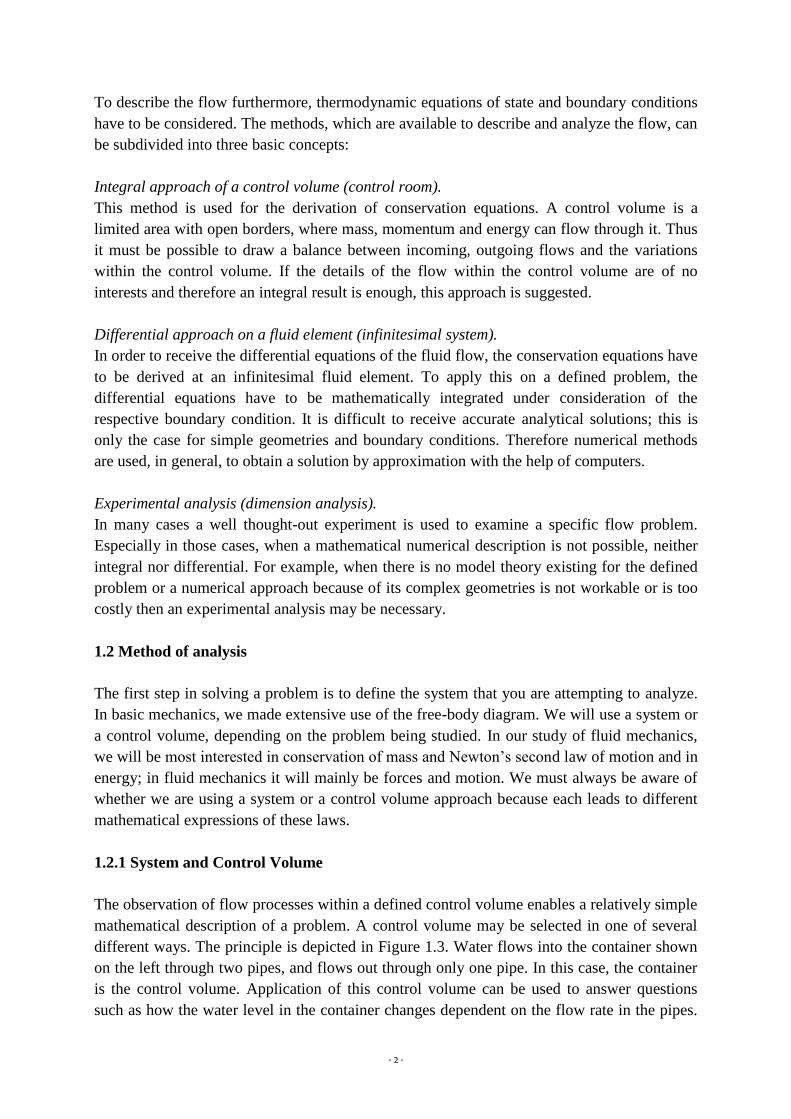
A control volume is an arbitrary volume in space through which fluid flows. The geometric
boundary of the control volume is called the control surface. The control surface may be real
or imaginary; it may be at rest or in motion. Figure 1.4 shows flow through a pipe junction,
with a control surface drawn on it. Note that some regions of the surface correspond to
physical boundaries (the walls of the pipe) and others (at locations 1, 2, and 3) are parts of the
surface that are imaginary (inlets or outlets). For the control volume defined by this surface,
we could write equations for the basic laws and obtain results such as the flow rate at outlet 3
given the flow rates at inlet and outlet 2, the force required to hold the junction in place, and
so on. It is always important to take care in selecting a control volume, as the choice has a big
effect on the mathematical form of the basic laws.
Figure 1.4 Fluid flow through a pipe junction.
1.3 Eulerian and Lagrangian Approach
Euler was born in Switzerland, in the town of Basel, on the 15th of April 1707. At that time,
Basel was one of the main centres of mathematics in Europe. At the age of 7, Euler started
school while his father hired a private mathematics tutor for him. At 13, Euler was already
attending lectures at the local university, and in 1723 gained his masters degree, with a

- 4 -
dissertation comparing the natural philosophy systems of Newton and Descartes. On his
father's wishes, Euler furthered his education by enrolling in the theological faculty, but
devoted all his spare time to studying mathematics. He wrote two articles on reverse trajectory
which were highly valued by his teacher Bernoulli. In 1727 Euler applied for a position as
physics professor at Basel university, but was turned down.
At this time a new centre of science had appeared in Europe - the Petersburg Academy of
Sciences. As Russia had few scientists of its own, many foreigners were invited to work at
this centre - among them Euler. On the 24th of May 1727 Euler arrived in Petersburg. His
great talents were soon recognised. Among the areas he worked in include his theory of the
production of the human voice, the theory of sound and music, the mechanics of vision, and
his work on telescopic and microscopic perception. On the basis of this last work, not
published until 1779, the construction of telescopes and microscopes was made possible.
Lagrange (1736-1813) was an Italian-French Mathematician and Astronomer. By the age of
18 he was teaching geometry at the Rotal Artillery School of Turin, where he organized
discussion group that became the Turin Academy of Sciences. In 1755, Lagrange sent Euler a
letter in which he discussed the Calculus of Variations. Euler was deeply impressed by
Lagrange's work, and he held back his own work on the subject to let Lagrange publish first.
When Euler left Berlin for St. Petersburg, he recommended that Lagrange succeed him as the
director of the Berlin Academy. Over the course of a long and celebrated career (he would be
lionized by Marie Antoinette, and made a count by Napoleon before his death), Lagrange
published a systemization of mechanics using his calculus of variations (Traité de mécanique
analytique), and did significant work on the three-body problem and astronomical
perturbations.
The studies carried out and shared by Euler and Lagrange can be seen from a web page of
http://eulerarchive.maa.org/correspondence/correspondents/Lagrange.html
Fluid mechanics problems can be regarded from two different points of view. First, the
Lagrangian approach, which tracks the individual particles (molecules) within the current.
The covered distance of such a particle is viewed as a function of the time. The Lagrangian
method is mainly used in the particle mechanics. Consider, for example, the application of
Newton’s second law to a particle of fixed mass. Mathematically, we can write Newton’s
second law for a system of mass m as
2
2
dt
rdm
dt
dvmmaF
We could use this Lagrangian approach to analyze a fluid flow by assuming the fluid to be
composed of a very large number of particles whose motion must be described. However,
keeping track of the motion of each fluid particle would become a horrendous bookkeeping
problem. Consequently, a particle description becomes unmanageable.
Often we find it convenient to use a different type of description. Particularly with control

- 5 -
volume analyses, it is convenient to use the field, or Eulerian, method of description, which
focuses attention on the properties of a flow at a given point in space as a function of time. In
the Eulerian method of description, the properties of a flow field are described as functions of
space coordinates and time. Thus, fluid dynamics measurements can be better accomplished
using the Eulerian approach. For example, to measure the velocity or the pressure in a tube
(flow), a measurement system is installed at a specific point (x,y,z) within it. The measuring
results then show a pressure field p(x,y,z) or a velocity field v(x,y,z). The velocity field is the
most important parameter of a current because other attributes are derivatives of it, e.g. the
transport of water, such as acceleration (a = dv/dt).
Figure 1.5 Streaklines over an automobiles.
1.4 Systems of Dimensions
Any valid equation that relates physical quantities must be dimensionally homogeneous; each
term in the equation must have the same dimensions. We recognize that Newton’s second law
(~F ~ m~a) relates the four dimensions, F, M, L, and t. Thus force and mass cannot both be
selected as primary dimensions without introducing a constant of proportionality that has
dimensions (and units). Length and time are primary dimensions in all dimensional systems in
common use. In some systems, mass is taken as a primary dimension. In others, force is
selected as a primary dimension.

- 6 -
Question 1-1
Determine the dimensions and units of the quantities given below?
Area, volume, velocity, angular velocity, acceleration, pressure, stress, energy, power,
density, dynamic viscosity and kinematic viscosity.
Solution 1-1
There are only four primary dimensions in fluid mechanics from which all other dimensions
can be derived. These are mass [M], length [L], time [T], temperature [Θ]. Secondary
dimensions are those derived as combinations of the primary dimensions, for example:
velocity, acceleration and force.
Newton’s Second Law: F= m x a
1 Newton Force= (1 kg) (m/sec2)
so dimensionally we can see that force has the units of mass times length divided by time
squared:
[F]=[MLT-2]
Secondary
Dimension
Primary
Components SI Unit
Area [L2] m2
Volume [L3] m3
Velocity [LT-1] m/s
Angular velocity [T-1] 1/s
Acceleration [LT-2] m/s2
Pressure or Stress [ML-1T-2] Pa=kg/(ms2)
Energy, Heat, Work [ML2T-2] J=Nm
Power [ML2T-3] W=J/s
Density [ML-3] kg/m3
Dynamic Viscosity [ML-1T-1] kg/(ms)
Kinematic Viscosity [L2T-1] m2/s
In engineering, we strive to make equations and formulas have consistent dimensions. That is,
each term in an equation, and obviously both sides of the equation, should be reducible to the
same dimensions. For example, a very important equation we will derive later on is the
Bernoulli equation
2
2
221
2
11
22z
g
V
g
Pz
g
V
g
P
which relates the pressure P, velocity V, and elevation z between points 1 and 2 along a
streamline for a steady, frictionless incompressible flow (density ρ). This equation is
dimensionally consistent because each term in the equation can be reduced to dimension of
[L]
Almost all equations you are likely to encounter will be dimensionally consistent. However,
you should be alert to some still commonly used equations that are not; these are often

- 7 -
“engineering” equations derived many years ago, or are empirical (based on experiment rather
than theory). For example, civil engineers often use the semi-empirical Manning equation:
n
SRV o
2132
1.5 Summary
In this chapter we introduced or reviewed a number of basic concepts and definitions,
including:
How fluids are defined, and the no-slip condition
System/control volume concepts
Lagrangian and Eulerian descriptions
Units and dimensions
Questions to solve:
1_For each quantity listed, indicate dimensions using mass as a primary dimension, and give
typical SI units:
(a) Power
(b) Pressure
(c) Modulus of elasticity
(d) Angular velocity
(e) Energy
(f) Moment of a force
(g) Momentum
(h) Shear stress
(i) Strain
(j) Angular momentum
2_For each quantity listed, indicate dimensions using force as a primary dimension, and give
typical SI units:
(a) Power
(b) Pressure
(c) Modulus of elasticity
(d) Angular velocity
(e) Energy
(f) Momentum
(g) Shear stress
(h) Angular momentum
3_The drag force FD on a body is given by
DD ACVF 2
2
1
Hence the drag depends on speed V, fluid density ρ, and body size (indicated by frontal area
A) and shape (indicated by drag coefficient CD). What are the dimensions of CD?
- 8 -
2. FUNDAMENTAL CONCEPTS IN FLUID MECHANICS
2.1 Fluid as a Continuum
As a consequence of the continuum assumption, each fluid property is assumed to have a
definite value at every point in space. Thus, the fluid properties such as density, temperature,
velocity, and so on are considered to be continuous functions of position and time. For
example, if density was measured simultaneously at an infinite number of points in the fluid
system, we would obtain an expression for the density distribution as a function of the space
coordinates at a given instant,
),,( zyx (2.1)
The density at a point may also vary with time (as a result of work done on or by the fluid
and/or heat transfer to the fluid). Thus the complete representation of density (the field
representation) is given by
),,,( tzyx (2.2)
Since density is a scalar quantity, requiring only the specification of a magnitude for a
complete description, the field represented by Equation (2.2) is a scalar field. An alternative
way of expressing the density of a substance (solid or fluid) is to compare it to an accepted
reference value, typically the maximum density of water, water (1000 kg/m3 at 4oC). Thus,
the specific gravity, SG, of a substance is expressed as
water
SG
(2.3)
For example, the SG of mercury is typically 13.6—mercury is 13.6 times as dense as water.
Appendix A contains specific gravity data for selected engineering materials. The specific
gravity of liquids is a function of temperature; for most liquids specific gravity decreases with
increasing temperature. The specific weight, γ, of a substance is another useful material
property. It is defined as the weight of a substance per unit volume and given as
V
mg (2.4)
For example, the specific weight of water is approximately 9.81 kN/m3.
2.2 Velocity Field
A very important property defined by a flow is the velocity field, given by
),,,( tzyxVV (2.5)
Velocity is a vector quantity, requiring a magnitude and direction for a complete description.
The velocity vector, V, also can be written in terms of its three scalar components.
wkvjuiV (2.6)
In general, each component, u, v, and w, will be a function of x, y, z, and t. Equation (2.5)
indicates the velocity of a fluid particle that is passing through the point x, y, z at time instant
t, in the Eulerian sense. We can keep measuring the velocity at the same point or choose any
other point x, y, z at the next time instant.

- 9 -
If properties at every point in a flow field do not change with time, the flow is termed steady.
Stated mathematically, the definition of steady flow is
0
t
where η represents any fluid property. Hence, for steady flow,
0
t
or ),,( zyx
and
0
t
V or ),,( zyxVV
In steady flow, any property may vary from point to point in the field, but all properties
remain constant with time at every point.
2.2.1 One, two and three dimensional flows
Although most flow fields are inherently three-dimensional, analysis based on fewer
dimensions is frequently meaningful. Consider, for example, the steady flow through a long
straight pipe that has a divergent section, as shown in Fig. 2.1 In this example, we are using
cylindrical coordinates (r, θ, x). We will learn in the next chapters that the velocity
distribution in this pipe may be described as
2
max 1R
ruu (2.7)
This is shown on the left of Fig. 2.1. The velocity u(r) is a function of only one coordinate,
and so the flow is one-dimensional. On the other hand, in the diverging section, the velocity
decreases in the x direction, and the flow becomes two-dimensional: ).( xruu
The term uniform flow field is used to describe a flow in which the velocity is constant. i.e.,
independent of all space coordinates, throughout the entire flow field.
Figure 2.1 Examples of one and two dimensional flows
- 10 -
2.3 Timelines, Pathlines, Streaklines and Streamlines.
If a number of adjacent fluid particles in a flow field are marked at a given instant, they form
a line in the fluid at that instant; this line is called a timeline. Subsequent observations of the
line may provide information about the flow field.
A pathline is the path or trajectory traced out by a moving fluid particle. To make a pathline
visible we might identify a fluid particle at a given instant.
Streamlines are lines drawn in the flow field so that at a given instant they are tangent to the
direction of flow at every point in the flow field. Since the streamlines are tangent to the
velocity vector at every point in the flow field, there can be no flow across a streamline.
Streamlines are the most commonly used visualization technique.
In steady flow the velocity at each point in the flow field remains constant with time and,
consequently the streamline shapes do not vary from one instant to the next. This implies that
a particle located on a given streamline will always move along the same streamline.
Furthermore, consecutive particles passing through a fixed point in space will be on the same
streamline and, subsequently, will remain on this streamline. Thus, in a steady flow, pathlines,
streaklines and streamlines are identical lines in the flow field.
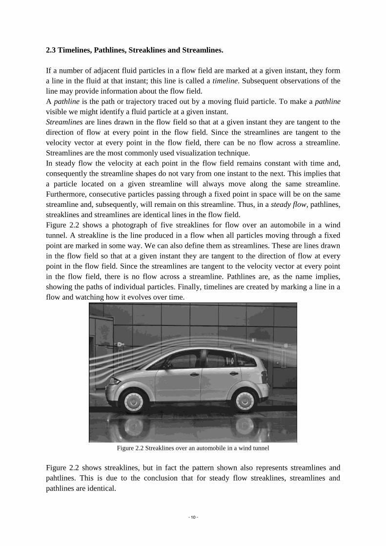
Figure 2.2 shows a photograph of five streaklines for flow over an automobile in a wind
tunnel. A streakline is the line produced in a flow when all particles moving through a fixed
point are marked in some way. We can also define them as streamlines. These are lines drawn
in the flow field so that at a given instant they are tangent to the direction of flow at every
point in the flow field. Since the streamlines are tangent to the velocity vector at every point
in the flow field, there is no flow across a streamline. Pathlines are, as the name implies,
showing the paths of individual particles. Finally, timelines are created by marking a line in a
flow and watching how it evolves over time.
Figure 2.2 Streaklines over an automobile in a wind tunnel
Figure 2.2 shows streaklines, but in fact the pattern shown also represents streamlines and
pahtlines. This is due to the conclusion that for steady flow streaklines, streamlines and
pathlines are identical.
- 11 -
We can use the velocity field to derive the shapes of streaklines, pathlines, and streamlines.
Starting with streamlines: Because the streamlines are parallel to the velocity vector, we can
write (for 2D)
),(
),(
yxu
yxv
dx
dy
streamline
(2.8)
Note that streamlines are obtained at an instant in time; if the flow is unsteady, time t is held
constant in Eq. 2.8. Solution of this equation gives the equation y=y(x), with an undetermined
integration constant, the value of which determines the particular streamline.
For pathlines (again considering 2D), we let x=xp(t) and y=yp(t) where xp(t) and yp(t) are the
instantaneous coordinates of a specific particle. We then get
),,( tyxudt
dx
particle
(2.9)
),,( tyxvdt
dy
particle
(2.10)
The simultaneous solution of these equations gives the path of a particle in parametric form
xp(t), yp(t).
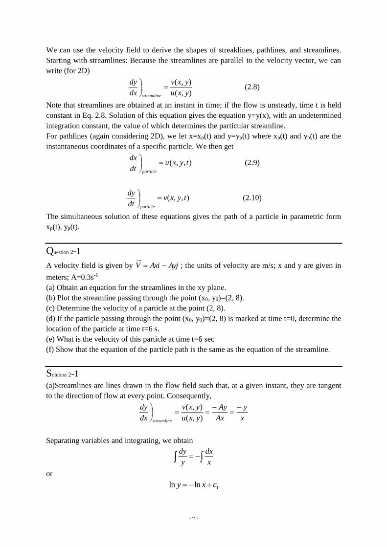
Question 2-1
A velocity field is given by AyjAxiV ; the units of velocity are m/s; x and y are given in
meters; A=0.3s-1
(a) Obtain an equation for the streamlines in the xy plane.
(b) Plot the streamline passing through the point (x0, y0)=(2, 8).
(c) Determine the velocity of a particle at the point (2, 8).
(d) If the particle passing through the point (x0, y0)=(2, 8) is marked at time t=0, determine the
location of the particle at time t=6 s.
(e) What is the velocity of this particle at time t=6 sec
(f) Show that the equation of the particle path is the same as the equation of the streamline.
Solution 2-1
(a)Streamlines are lines drawn in the flow field such that, at a given instant, they are tangent
to the direction of flow at every point. Consequently,
x
y
Ax
Ay
yxu
yxv
dx
dy
streamline
),(
),(
Separating variables and integrating, we obtain
x
dx
y
dy
or
1lnln cxy

- 12 -
This can be written as xy=c
(b) For the streamline passing through the point (x0, y0) = (2, 8) the constant, c, has a value of
16 and the equation of the streamline through the point (2, 8) is 2
00 16myxxy
The plot is as sketched below.
(c) The velocity field is AyjAxiV . At the point (2, 8) the velocity is
jimjisyjxiAV 4.26.0)82(3.0)( 1 m/sec
(d) A particle moving in the flow field will have velocity given by
AyjAxiV
Thus
Axdt
dxu p and Ay
dt
dyv p
Separating variables and integrating (in each equation) gives
tx
x
Adtx
dx
o 0
and
ty
y
Adty
dy
o 0
Then
Atx
x
o
ln and Aty
y
o
ln
or At
oexx and At
oeyy

- 13 -
At t=6 sec,
mex 1.12)2( 6)3.0( and mey 31.1)8( 6)3.0(
At t=6 sec, the particle is at (12.1, 1.32)m
(e) At the point (12.1, 1.32) m,
jimjisyjxiAV 396.063.3)32.11.12(3.0)( 1 m/sec
(f) To determine the equation of the pathline, we use the parametric Equations At
oexx and At
oeyy
and eliminate t. Solving for eAt from both equations
o
oAt
x
x
y
ye
Therefore 216myxxy oo
2.4 Stress Field.
In our study of fluid mechanics, we will need to understand what kinds of forces act on fluid
particles. Each fluid particle can experience: surface forces (pressure, friction) that are
generated by contact with other particles or a solid surface; and body forces (such as gravity
and electromagnetic) that are experienced throughout the particle. The gravitational body
force acting on an element of volume, dV, is given by ρgdV where ρ is the density (mass per
unit volume) and g is the local gravitational acceleration. Thus the gravitational body force
per unit volume is ρg and the gravitational body force per unit mass is g.
Surface forces on a fluid particle lead to stresses. The concept of stress is useful for describing
how forces acting on the boundaries of a medium (fluid or solid) are transmitted throughout
the medium. The difference between a fluid and a solid is, as we’ve seen, that stresses in a
fluid are mostly generated by motion rather than by deflection.
Imagine the surface of a fluid particle in contact with other fluid particles, and consider the
contact force being generated between the particles. We consider the stress on the element
δAx, whose outwardly drawn normal is in the x direction. The force, δF, has been resolved
into components along each of the coordinate directions. Dividing the magnitude of each
force component by the area, δAx, and taking the limit as δAx approaches zero, we define the
three stress components shown in Fig. 2.3.
Referring to the infinitesimal element as shown in Fig. 2.4, we see that there are six planes
(two x planes, two y planes, and two z planes) on which stresses may act. In order to
designate the plane of interest, we could use terms like front and back, top and bottom, or left
and right. However, it is more logical to name the planes in terms of the coordinate axes. The
planes are named and denoted as positive or negative according to the direction of the
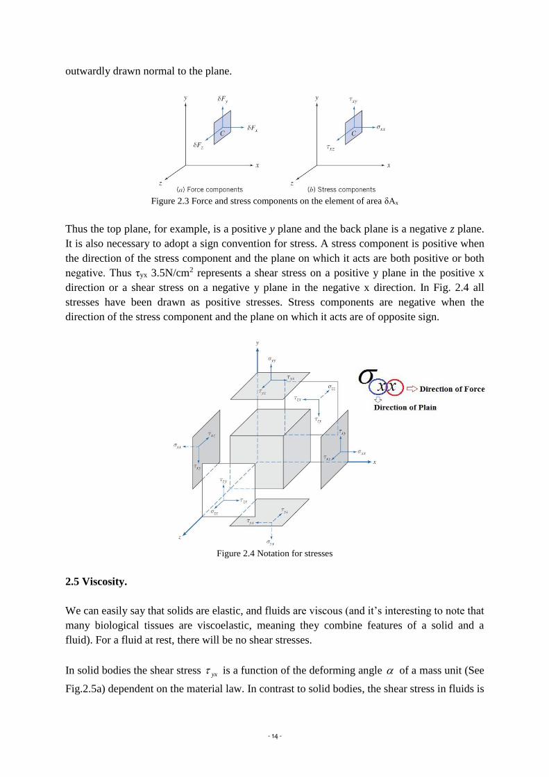
- 14 -
outwardly drawn normal to the plane.
Figure 2.3 Force and stress components on the element of area δAx
Thus the top plane, for example, is a positive y plane and the back plane is a negative z plane.
It is also necessary to adopt a sign convention for stress. A stress component is positive when
the direction of the stress component and the plane on which it acts are both positive or both
negative. Thus τyx 3.5N/cm2 represents a shear stress on a positive y plane in the positive x
direction or a shear stress on a negative y plane in the negative x direction. In Fig. 2.4 all
stresses have been drawn as positive stresses. Stress components are negative when the
direction of the stress component and the plane on which it acts are of opposite sign.
Figure 2.4 Notation for stresses
2.5 Viscosity.
We can easily say that solids are elastic, and fluids are viscous (and it’s interesting to note that
many biological tissues are viscoelastic, meaning they combine features of a solid and a
fluid). For a fluid at rest, there will be no shear stresses.
In solid bodies the shear stress yx is a function of the deforming angle of a mass unit (See
Fig.2.5a) dependent on the material law. In contrast to solid bodies, the shear stress in fluids is
- 15 -
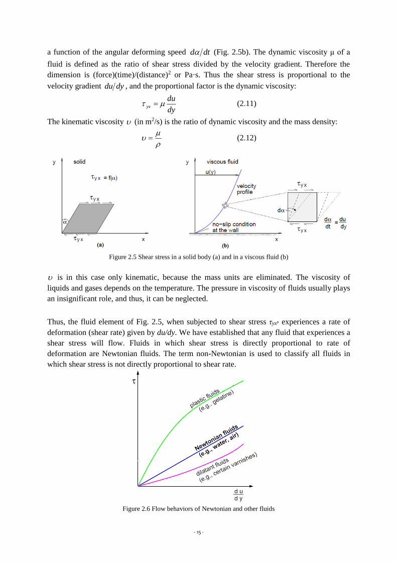
a function of the angular deforming speed dtd (Fig. 2.5b). The dynamic viscosity μ of a
fluid is defined as the ratio of shear stress divided by the velocity gradient. Therefore the
dimension is (force)(time)/(distance)2 or Pa·s. Thus the shear stress is proportional to the
velocity gradient dydu , and the proportional factor is the dynamic viscosity:
dy
duyx (2.11)
The kinematic viscosity (in m2/s) is the ratio of dynamic viscosity and the mass density:
(2.12)
Figure 2.5 Shear stress in a solid body (a) and in a viscous fluid (b)
is in this case only kinematic, because the mass units are eliminated. The viscosity of
liquids and gases depends on the temperature. The pressure in viscosity of fluids usually plays
an insignificant role, and thus, it can be neglected.
Thus, the fluid element of Fig. 2.5, when subjected to shear stress τyx, experiences a rate of
deformation (shear rate) given by du/dy. We have established that any fluid that experiences a
shear stress will flow. Fluids in which shear stress is directly proportional to rate of
deformation are Newtonian fluids. The term non-Newtonian is used to classify all fluids in
which shear stress is not directly proportional to shear rate.
Figure 2.6 Flow behaviors of Newtonian and other fluids

- 16 -
Note that, since the dimensions of τ are [F/L2] and the dimensions of du/dy are [1/t], μ has
dimensions [Ft/L2]. Since the dimensions of force, F, mass,M, length, L, and time, t, are
related by Newton’s second law of motion, the dimensions of μ can also be expressed as
[M/Lt]. The calculation of viscous shear stress is illustrated in the following question.
Question 2-2
An infinite plate is moved over a second plate on a layer of liquid as shown. For small gap
width, d, we assume a linear velocity distribution in the liquid. The liquid viscosity is 0.0065
g/cm.s and its specific gravity is 0.88.
Determine:
(a) The viscosity of the liquid, in N s/m2.
(b) The kinematic viscosity of the liquid, in m2/s.
(c) The shear stress on the upper plate, in N/m2.
(d) The shear stress on the lower plate, in Pa.
(e) The direction of each shear stress calculated in parts (c) and (d).
Solution 2-2
Given: Linear velocity profile in the liquid between infinite parallel plates are as shown.
μ = 0:0065 g/cm.s
SG = 0:88
Find:
(a) μ in units of N s/m2
(b) ν in units of m2/s.
(c) τ on upper plate in units of N/m2
(d) τ on lower plate in units of Pa.
(e) Direction of stresses in parts (c) and (d).
Governing equation: dy
du in which
Assumptions: (1) Linear velocity distribution (given)
(2) Steady flow
(3) μ=constant

- 17 -
m
cm
g
kg
scm
g 100
1000
1
.0065.0
sec./105.6 4 mkg
Convert the kilograms into Newton by using the Newtons Second Law
2sec/
11
m
Newtonkg
kgm
N
sm
kg 1
sec/
1
.00065.0
2
24 /.105.6 msN
OHSG2
3
24
1000)88.0(
/.105.6
2mkg
msN
SG OH
sm /1039.7 27
dydy
du
Since u varies linearly with respect to y,
d
U
d
U
y
u
dy
du
0
0
1100010003.0
13.0 s
m
mm
mms
m
224 /65.01000
/.105.6 mNs
msNd
Uupper
PaN
mPamN
d
Ulower 65.0
./65.0
22
Directions of shear stresses on upper and lower plates are as shown in the figure below. The
upper plate is a negative y surface; so positive τ acts in the negative x direction. The lower
plate is a positive y surface; so positive τ acts in the positive x direction.

- 18 -
2.6 Description and Classification of Fluid Motions.
Fluid mechanics is a huge discipline; it covers everything from the aerodynamics of a
supersonic transport vehicle to the lubrication of human joints by fluid. We need to break
fluid mechanics down into manageable proportions. It turns out that the two most difficult
aspects of a fluid mechanics analysis to deal with are: (1) the fluid’s viscous nature and (2) its
compressibility. In fact, the area of fluid mechanics theory that first became highly developed
was that dealing with a frictionless incompressible fluid. Although not the only way to do so,
most engineers subdivide fluid mechanics in terms of whether or not viscous effects and
compressibility effects are present.
Viscous and Inviscid Flows.
When two fluid layers move relative to each other, a friction force develops between them
and the slower layer tries to slow down the faster layer. This internal resistance to flow is
quantified by the fluid property viscosity, which is a measure of internal stickiness of the
fluid. Viscosity is caused by cohesive forces between the molecules in liquids and by
molecular collisions in gases. There is no fluid with zero viscosity, and thus all fluid flows
involve viscous effects to some degree. However, in many flows of practical interest, there are
regions (typically regions not close to solid surfaces) where viscous forces are negligibly
small compared to inertial or pressure forces. Neglecting the viscous terms in such inviscid
flow regions greatly simplifies the analysis without much loss in accuracy.
The development of viscous and inviscid regions of flow as a result of inserting a flat plate
parallel into a fluid stream of uniform velocity is shown in Figure 2.7. The fluid sticks to the
plate on both sides because of the no-slip condition, and the thin boundary layer in which the
viscous effects are significant near the plate surface is the viscous flow region. The region of
flow on both sides away from the plate and unaffected by the presence of the plate is the
inviscid flow region.
Figure 2.7 Viscous and inviscid flow conditions
We can estimate whether or not viscous forces, as opposed pressure forces, are negligible by
simply computing the Reynolds number.
VLRe (2.13)
Where ρ and μ are the fluid density and viscosity, respectively, and V and L are the typical or
characteristic velocity and size scale of the flow, respectively. The Reynolds number can be

- 19 -
interpreted as the ratio of momentum (or inertia) to viscous forces. If the Reynolds number is
large viscous effects will be negligible at least in most of the flow; if the Reynolds number is
small, viscous effects will be dominant. Finally, if the Reynolds number is neither large nor
small, no general conclusions can be drawn.
Prandtl suggested that even though friction is negligible in general for high Reynolds number
flows, there will always be a thin boundary layer, in which friction is significant and across
the width of which the velocity increases rapidly from zero (at the surface) to the value
inviscid flow theory predicts (on the outer edge of the boundary layer). This is shown in more
detail in Figure 2.8.
Figure 2.8 Schematic drawing of a boundary layer
Laminar and Turbulent Flows.
There are two kinds of fluid (liquids and gases) flow that are observed: laminar (streamline)
flow and turbulent flow. Particles of a continuous fluid can be considered to travel along
smooth continuous paths which are given the name streamlines. These streamlines can be
curved or straight, depending on the flow of the fluid. This type of motion is also called
laminar flow. This continuous substance can be regarded as being made up of bundles or
tubes of streamlines (flow tubes). The tubes have elastic properties:
A tensile strength which means that the parts of the fluid along a particular streamline
stick together and do not separate from one another.
Zero shear modulus, which means that each streamline moves independently of any
other.
Streamline motion is not the only possible kind of fluid motion. When the motion becomes
too violent, eddies and vortices occur. The motion becomes turbulent. Turbulence is important
because it is a means whereby energy gets dissipated. The shape of a body will, to some
extent, decide whether it will move through a fluid in streamline or turbulent motion.

- 20 -
Figure 2.9 Schematic drawing of a laminar and turbulent flow conditions
In laminar flow the flow separates into "layers" that slide relative to one another without
mixing. If we introduce a coloured stream into the laminar flow, the colour will stay in the
stream. The flow is called steady. Laminar flow can be represented by a set of lines known as
streamlines (flow lines).
• An individual particle will follow a streamline.
• The flow pattern does not change with time. All particles starting on a streamline will
continue to move on that streamline.
• A set of streamlines is called a flow tube.
• Streamlines can't cross nor intersect the "walls" of the flow tube.
• The instantaneous velocity of the particle is in the direction of the tangent to the streamline.
When the turbulence dominates, a vigorous mixing (stirring) of the fluid occurs. A complex
flow pattern changes continuously with time. The velocity of the particles at each given point
varies chaotically with time. A coloured dye added to a stream will readily disperse very
suddenly as the flow rate increases. The flow becomes unstable at some critical speed.
Figure 2.10 The laminar and turbulent flow conditions for dye injected into pipe by tube

- 21 -
Compressible and Incompressible Flows.
Flows in which variations in density are negligible are termed incompressible; when density
variations within a flow are not negligible, the flow is called compressible. The most common
example of compressible flow concerns the flow of gases, while the flow of liquids may
frequently be treated as incompressible. For many liquids, density is only a weak function of
temperature. At modest pressures, liquids may be considered incompressible. However, at
high pressures, compressibility effects in liquids can be important. Pressure and density
changes in liquids are related by the bulk compressibility modulus, or modulus of elasticity,
d
dpEv (2.14)
The modulus of elasticity of water is Ev≈ 2.1x10⁹ N/m2. Hence, to compress a water volume
only about 1%, the pressure has to be increased by approximately 200bar. Therefore, in most
cases, water flow can be considered as incompressible. This is also applicable to most other
liquid flow systems.
Question 2-3
What is the pressure at a depth of 10,000 meters in water if the bulk modulus of elasticity of
water is 2.1x10⁹ N/m2 and the pressure of water at any depth can be calculated by the static
fluid pressure formula? Also calculate the change in density of water at the same depth.
ghP
Solution 2-3
Given: Ev= 2.1x10⁹ N/m2 and depth is 10,000 meters
Find: Pressure and density of water at a depth of 10,000 meters.
Apply pressure equation.
ghP
1000081.91000 P 2/1.98 mMNP
Pressure and density changes in liquids are related by the bulk compressibility modulus, or
modulus of elasticity,
d
dpEv
047.0101.2
101.989
6
vE
dpd
Therefore, the density of water at a depth of 10,000 meters is about 1000 + 47 = 1047 kg/m3
- 22 -
That proves the incompressibility of the water.
2.7 Summary
In this chapter we have completed our review of some of the fundamental concepts we will
utilize in our study of fluid mechanics. Some of these are:
How to describe flows (timelines, pathlines, streamlines, streaklines).
Forces (surface, body) and stresses (shear, normal).
Types of fluids (Newtonian, non-Newtonian and viscosity
Types of flow (viscous/inviscid, laminar/turbulent, compressible/incompressible).
Questions to solve:
1_The velocity for a steady, incompressible flow in the xy plane is given by
jx
Ayi
x
AV
2
where A=2 m2/s, and the coordinates are measured in meters. Obtain an equation for the
streamline that passes through the point (x, y) = (1, 3). Calculate the time required for a fluid
particle to move from x=1 m to x=2 m in this flow field.
2_A flow field is given by ,
AyjAxiV 2
where A=2 s-1. Verify that the parametric equations for particle motion are given by xp=c1eAt
and yp=c2e2At. Obtain the equation for the pathline of the particle located at the point (x, y) =
(2, 2) at the instant t=0. Compare this pathline with the streamline through the same point.
3_The velocity distribution for laminar flow between parallel plates is given by 2
max
21
h
y
u
u
where h is the distance separating the plates and the origin is placed midway between the
plates. Consider a flow of water, with umax=0.10 m/s and h=0.1 mm. Calculate the shear stress
on the upper plate and give its direction. Sketch the variation of shear stress across the
channel. The dynamic viscosity of the fluid is 1.14x10⁻³ Nsec/m2.
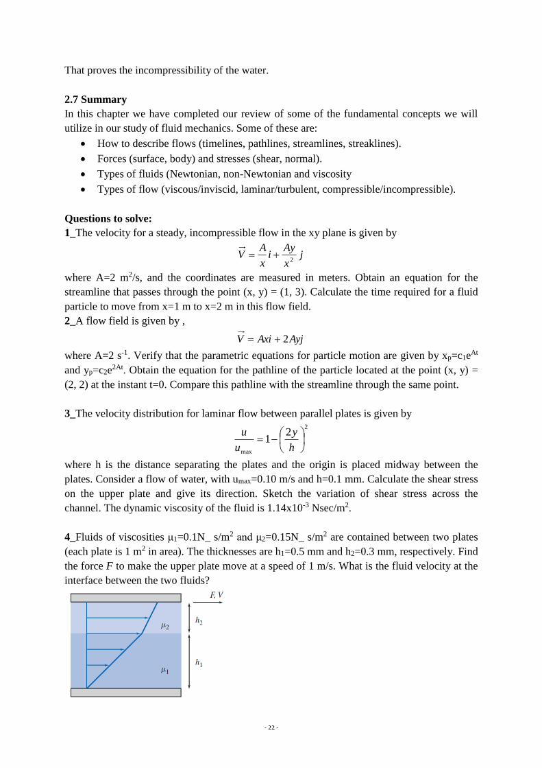
4_Fluids of viscosities μ1=0.1N_ s/m2 and μ2=0.15N_ s/m2 are contained between two plates
(each plate is 1 m2 in area). The thicknesses are h1=0.5 mm and h2=0.3 mm, respectively. Find
the force F to make the upper plate move at a speed of 1 m/s. What is the fluid velocity at the
interface between the two fluids?

- 23 -
5_ The viscous boundary layer velocity profile shown in the following figure can be
approximated by a parabolic equation, 2
)(
yc
ybayu
The boundary condition is u=U (the free stream velocity) at the boundary edge δ (where the
viscous friction becomes zero). Find the values of a, b, and c.
6_ What is the Reynolds number of water at 20oC flowing at 0.25 m/s through a 5-mm-
diameter tube? If the pipe is now heated, at what mean water temperature will the flow
transition to turbulence? Assume the velocity of the flow remains constant.

- 24 -
3. FLUID STATICS
3.1 The Basic Equation of Fluid Statics
In a static fluid there are no shear stresses, so the only surface force is the pressure force
(which is a kind of compression force). Pressure is a scalar field, p=p(x, y, z); in general we
expect the pressure to vary with position within the fluid. The net pressure force that results
from this variation can be found by summing the forces that act on the six faces of the fluid
element.
The pressure forces acting on the dydz plane of the differential element are shown in Fig. 3.1.
Each pressure force is the magnitude of the pressure. This magnitude is multiplied by the area
of the face to give the magnitude of the pressure force. Note also in Fig. 3.1 that the pressure
force on each face acts against the face. A positive pressure corresponds to a compressive
normal stress. Pressure forces on the other faces of the element are obtained in the same way.
Combining all such forces gives the net surface force acting on the element.
Figure 3.1 Differential fluid element and pressure forces in the y direction
The total force applied on the surface can be written in terms of surface forces and body
forces. The body force is the weight of the differential element in the negative y-direction.
gdVFd B
In which g represents the unit weight of the differential element and dV represents the
volume of the element. As a result the body force for the differential element can be written as
gdxdydzWeightFd B
The surface forces can be written in all the three directions as:
0
dzdydx
x
PPdzdyP x
xx in x direction
0
dzdxdy
y
PPdzdxP
y
yy in y direction
0
dxdydz
z
PPdxdyP z
zz in z direction
Adding all the surface forces in all the three directions is therefore results in
dxdzdyz
P
y
P
x
P zyx

- 25 -
Summing all the surface forces and body forces applied on a differential element the resultant
equation will form:
gdxdzdydxdzdyz
P
y
P
x
PFdFdFd zyx
BS
Since the fluid is in static equilibrium, all the forces must be equal to zero. Therefore, total
forces in all the three directions can be written as
0
dxdzdygdxdzdy
x
PFdFdFd x
xBS (3.1a)
0
dxdzdygdxdzdy
y
PFdFdFd y
y
BS (3.1b)
0
dxdzdygdxdzdy
z
PFdFdFd z
zBS (3.1c)
Equations 3.1a,b,c describe the pressure variation in each of the three coordinate directions in
a static fluid. It is convenient to choose a coordinate system such that the gravity vector is
aligned with one of the coordinate axes. If the coordinate system is chosen with the y-axis
directed vertically upward, as in Fig. 3.1, then gx=0, gy=-g, and gz=0. Under these conditions,
the component equations become
0
x
p g
y
p
0
z
p (3.2)
Equations 3.2 indicate that, under the assumptions made, the pressure is independent of
coordinates x and z; it depends on y alone. Thus since P is a function of a single variable, a
total derivative may be used instead of a partial derivative. With these simplifications, Eqs.
3.1 and 3.2 finally reduce to
gdy
dp (3.3)
Restrictions: (1) Static fluid. (2) Gravity is the only body force. (3) The y-axis is vertical and
upward. In Eq. 3.3, γ is the specific weight of the fluid. This equation is the basic pressure
height relation of fluid statics. It is subject to the restrictions noted. Therefore, it must be
applied only where these restrictions are reasonable for the physical situation. To determine
the pressure distribution in a static fluid, Eq. 3.3 may be integrated and appropriate boundary
conditions applied. Before considering specific applications of this equation, it is important to
remember that pressure values must be stated with respect to a reference level. If the reference
level is a vacuum, pressures are termed absolute, as shown in Fig. 3.2. Most pressure gages
indicate a pressure difference—the difference between the measured pressure and the ambient
level (usually atmospheric pressure). Pressure levels measured with respect to atmospheric
pressure are termed gage pressures. Thus

- 26 -
Figure 3.2 Absolute and gage pressures, showing reference levels
3.2 Pressure variation in a Static Fluid
We proved that pressure variation in any static fluid is described by the basic pressure height
relation,
gdy
dp
Although ρg may be defined as the specific weight, γ, it has been written as ρg in Eq. 3.3 to
emphasize that both ρ and g must be considered variables. In order to integrate Eq. 3.3 to find
the pressure distribution, we need information about variations in both ρ and g. For most
practical engineering situations, the variation in g is negligible. Only for a purpose such as
computing very precisely the pressure change over a large elevation difference would the
variation in g need to be included. Unless we state otherwise, we shall assume g to be constant
with elevation at any given location.
Incompressible Liquids: Manometers
The following Equation (3.4) indicates that the pressure difference between two points in a
static incompressible fluid can be determined by measuring the elevation difference between
the two points. Devices used for this purpose are called manometers.
ghppp o (3.4)
To consider the above equation, we have to prove Euler’s Condition of Equilibrium. The cube
dx.dy.dz of the fluid sample at rest must have the mass forces and the pressure on the surface
in equilibrium.
Let us consider a mass in static water whose volume is:
dzvolume .1.1 and the total depth of water is
yzH
- 27 -
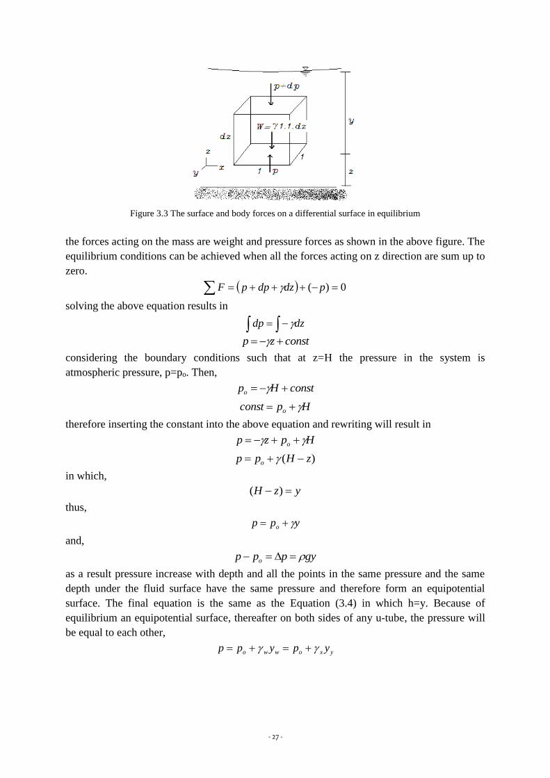
Figure 3.3 The surface and body forces on a differential surface in equilibrium
the forces acting on the mass are weight and pressure forces as shown in the above figure. The
equilibrium conditions can be achieved when all the forces acting on z direction are sum up to
zero.
0)( pdzdppF
solving the above equation results in
dzdp
constzp considering the boundary conditions such that at z=H the pressure in the system is
atmospheric pressure, p=po. Then,
constHpo
Hpconst o
therefore inserting the constant into the above equation and rewriting will result in
Hpzp o
)( zHpp o
in which,
yzH )(
thus,
ypp o
and,
gyppp o
as a result pressure increase with depth and all the points in the same pressure and the same
depth under the fluid surface have the same pressure and therefore form an equipotential
surface. The final equation is the same as the Equation (3.4) in which h=y. Because of
equilibrium an equipotential surface, thereafter on both sides of any u-tube, the pressure will
be equal to each other,
yxowwo ypypp

- 28 -
Question 3-1
Normal blood pressure for a human is 120/80 mm Hg. By modelling a sphygmomanometer
pressure gage as a U-tube manometer, convert these pressures to kPa. Note that the specific
gravity of mercury, SGHg=13.6 and density of water is, ρH2O = 1000 kg/m3
Solution 3-1
Given: Gage pressures of 120 and 80 mm Hg.
Find: The corresponding pressures in kPa
Solution:
Apply hydrostatic equation to points A, A’, and B.
Governing equation:
ghppp o
Assumptions:
(1) Static fluid.
(2) Incompressible fluids.
(3) Neglect air density (<< Hg density).
Applying the governing equation between points A’ and B (and pB is atmospheric and
therefore zero gage):
ghSGghpp OHHgHgBA 2'
In addition, the pressure increases as we go downward from point A’ to the bottom of the
manometer, and decreases by an equal amount as we return up the left branch to point A. This
means points A and A’ have the same pressure, so we end up with
ghSGpp OHHgAA 2'
Substituting SGHg=13.6 and ρH2O = 1.000 kg/m3 yields for the systolic pressure (h=120 mm
Hg)
mkg
sN
mm
mmm
s
m
m
kgpp Asystolic
.
.
100012081.910006.13
2
23
- 29 -
kPam
Npsystolic 16000,16
2
By a similar process, the diastolic pressure (h=80 mm Hg) is
kPapsystolic 67.10
Note:
Two points at the same level in a continuous single fluid have the same pressure.
In manometer problems we neglect change in pressure with depth for a gas: ρgas <<
ρliquid.
This problem shows the conversion from mm Hg to kPa. More generally, 1 atm = 101
kPa = 760 mm Hg.
Manometers are simple and inexpensive devices used frequently for pressure measurements.
Because the liquid level change is small at low pressure differential, a U-tube manometer may
be difficult to read accurately.
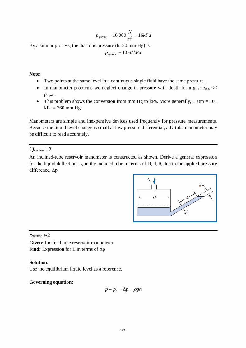
Question 3-2
An inclined-tube reservoir manometer is constructed as shown. Derive a general expression
for the liquid deflection, L, in the inclined tube in terms of D, d, θ, due to the applied pressure
difference, Δp.
Solution 3-2
Given: Inclined tube reservoir manometer.
Find: Expression for L in terms of Δp
Solution:
Use the equilibrium liquid level as a reference.
Governing equation:
ghppp o

- 30 -
Assumptions:
(1) Static fluid.
(2) Incompressible fluids.
Applying the governing equation between
points 1 and 2:
)( 2121 hhgppp liquid
To eliminate h1, we recognize that the volume of manometer liquid remains constant; the
volume displaced from the reservoir must equal the volume that rises in the tube, so
Ld
hD
44
2
1
2 or
2
2
1D
dLh
In addition, from the geometry of the manometer, h2=L sin θ. Substituting into the governing
equations:
22
sinsinD
dgL
D
dLLgp liquidliquid
Thus
2
sinD
dg
pL
liquid
Students sometimes have trouble analysing multiple-liquid manometer situations. The
following rules of thumb are useful:
1. Any two points at the same elevation in a continuous region of the same liquid are at
the same pressure.
2. Pressure increases as one goes down a liquid column.
To find the pressure difference Δp between two points separated by a series of fluids, we can
use the following modification of
ghppp o
which can be written as
ii hgp (3.5)
where ρi and hi represent the densities and depths of the various fluids, respectively. Use care
in applying signs to the depths hi; they will be positive downwards, and negative upwards.
Question 3-3 illustrates the use of a multiple-liquid manometer for measuring a pressure
difference.

- 31 -
Question 3-3
Water flows through pipes A and B. Lubricating oil is in the upper portion of the inverted U.
Mercury is in the bottom of the manometer bends. Determine the pressure difference, pA-pB,
in units of kPa.
Solution 3-3
Given: Multiple liquid manometer as shown
Find: Pressure difference, pA-pB in kPa
Solution:
Governing equation:
ii hgp and water
SG
Assumptions:
(1) Static fluid.
(2) Incompressible fluids.
Applying the governing
equation working from point
B to A:
12345 22dddddgppp OHHgoilHgOHBA
This equation can also be derived by repeatedly using
)( 1212 hhgppp
Beginning at point C and applying the equation between successive points along the
manometer gives
12dgpp OHAC which results 12
dgpp OHAC
2dgpp HgDC which results 2dgpp HgCD
3dgpp oilDE which results 3dgpp oilDE

- 32 -
4dgpp HgFE which results 4dgpp HgEF
52dgpp OHBF which results 52
dgpp OHFB
Multiplying each equation by minus one and adding, we obtain:
BFFEEDDCCABA PPPPPPPPPPpp
54321 22dgdgdgdgdgpp OHHgoilHgOHBA
Substituting oHSG2
with SGHg=13.6 and SGoil = 0.88 yields
54321 222226.1388.06.13 dddddgpp OHOHOHOHOHBA
54321 6.1388.06.132
dddddgpp OHBA
mmgpp OHBA 20017008810202502
mmgpp OHBA 25822
mkg
sNm
m
kg
s
mpp BA
.
.1
10002582100081.9
2
32
kPapp BA 33.25
3.3 Hydrostatic Forces on Submerged Surfaces
Now that we have determined how the pressure varies in a static fluid, we can examine the
force on a surface submerged in a liquid. In order to determine completely the resultant force
acting on a submerged surface, we must specify:
1. The magnitude of the force
2. The direction of the force
3. The line of action of the force
We shall consider both plane and curved submerged surface.
Hydrostatic Force on a plane Submerged Surfaces
A plane submerged surface, on whose upper face we wish to determine the resultant
hydrostatic force, is shown in Figure 3.4 The coordinates are important: They have been
chosen so that the surface lies in the xy plane, and the origin O is located at the intersection of
the plane surface (or its extension) and the free surface. As well as the magnitude of the force
FR, we wish to locate the point (with coordinates x’, y’) through which it acts on the surface.
Since there are no shear stresses in a static fluid, the hydrostatic force on any element of the
surface acts normal to the surface. The pressure force acting on an element dA=(dx)(dy) of
the upper surface is given by
pdAdF

- 33 -
The resultant force acting on the surface is found by summing the contributions of the
infinitesimal forces over the entire area. Usually when we sum forces we must do so in a
vectorial sense. However, in this case all of the infinitesimal forces are perpendicular to the
plane, and hence so is the resultant force. Its magnitude is given by
A
R pdAF (3.6)
Figure 3.4 Plane submerged surface
In order to evaluate the integral in Eq. 3.6, both the pressure, p, and the element of area, dA,
must be expressed in terms of the same variables. We can use Eq. 3.4 to express the pressure
p at depth h in the liquid as
ghpp o
In this expression po is the pressure at the free surface (h=0). In addition, we have, from the
system geometry, h=y sin θ. Using this expression and the above expression for pressure in
Eq. 3.6,
A
o
A
o
A
R dAgypdAghppdAF )sin()(
A
o
AA
oR ydAgApydAgdApF sinsin
The integral is the first moment of the surface area about the x axis, which may be written as
AyydA c
A
where yc is the y coordinate of the centroid of the area, A. Thus,
AygApF coR sin
AghpF coR )(
ApF cR (3.7)
where pc is the absolute pressure in the liquid at the location of the centroid of area A.
Equation 3.7 computes the resultant force due to the liquid—including the effect of the
ambient pressure po—on one side of a submerged plane surface. It does not take into account

- 34 -
whatever pressure or force distribution may be on the other side of the surface. However, if
we have the same pressure, po, on this side as we do at the free surface of the liquid, as shown
in Fig. 3.5, its effect on FR cancels out, and if we wish to obtain the net force on the surface
we can use Eq. 3.7 with pc expressed as a gage rather than absolute pressure. In computing FR
we can use either the integral of Eq. 3.6 or the resulting Eq. 3.7. It is important to note that
even though the force can be computed using the pressure at the center of the plate, this is not
the point through which the force acts! Our next task is to determine (x’,y’), the location of
the resultant force. Let’s first obtain y’ by recognizing that the moment of the resultant force
about the x axis must be equal to the moment due to the distributed pressure force. Taking the
sum (i.e., integral) of the moments of the infinitesimal forces dF about the x axis we obtain
Figure 3.5 Pressure distribution on plane submerged structure
A
R ypdAFy (3.8)
We can integrate by expressing p as a function of y as before:
A
o
A
o
A
R dAgyypdAghpyypdAFy )sin()( 2
AA
oR dAygydApFy 2sin
The first integral is our familiar ycA. The second integral,
A
dAy 2
is the second moment of area about the x axis, Ixx. We can use the parallel axis theorem, 2
cxxxx AyII
to replace Ixx with the standard second moment of area, about the centroidal x’ axis.
Using all of these, we find
xxcoccxxcoR IgAgypyAyIgAypFy sin)sin()(sin 2
xxRcxxcocR IgFyIgAghpyFy sinsin)(
Finally we obtain for y’:
R
xxc
F
Igyy
sin (3.9)
Equation 3.9 is convenient for computing the location y’ of the force on the submerged side of
the surface when we include the ambient pressure po. If we have the same ambient pressure

- 35 -
acting on the other side of the surface we can use Eq. 3.7 with po neglected to compute the net
force,
AgyAyghApF ccccR gage sin
and Eq. 3.9 becomes for this case
c
xxc
Ay
Iyy (3.10)
Equation 3.8 is the integral equation for computing the location y’ of the resultant force; Eq.
3.9 is a useful algebraic form for computing y’ when we are interested in the resultant force
on the submerged side of the surface; Eq. 3.10 is for computing y’ when we are interested in
the net force for the case when the same po acts at the free surface and on the other side of the
submerged surface. For problems that have a pressure on the other side that is not po, we can
either analyze each side of the surface separately or reduce the two pressure distributions to
one net pressure distribution, in effect creating a system to be solved using Eq. 3.7 with pc
expressed as a gage pressure.
Note that in any event, y’> yc—the location of the force is always below the level of the plate
centroid. This makes sense—as Fig. 3.5 shows, the pressures will always be larger on the
lower regions, moving the resultant force down the plate.
A similar analysis can be done to compute x’, the x location of the force on the plate. Taking
the sum of the moments of the infinitesimal forces dF about the y axis we obtain
A
R xpdAFx (3.11)
A
o
A
o
A
R dAgxyxpdAghpxxpdAFx )sin()(
AA
oR xydAgxdApFx sin
The first integral is xcA(where xc is the distance of the centroid from y axis). The second
integral is
xy
A
IxydA
Using the parallel axis theorem,
ccyxxy yAxII
we find
yxcocccyxcoR IgAgypxyAxIgAxpFx sin)sin()(sin
yxRcyxcocR IgFxIgAghpxFy sinsin)(
Finally we obtain for x’

- 36 -
R
yx
cF
Igxx
sin (3.12)
Equation 3.12 is convenient for computing x’ when we include the ambient pressure po. If we
have ambient pressure also acting on the other side of the surface we can again use Eq. 3.7
with po neglected to compute the net force and Eq. 3.12 becomes for this case
c
yx
cAy
Ixx
(3.13)
Equation 3.11 is the integral equation for computing the location x’ of the resultant force; Eq.
3.12 can be used for computations when we are interested in the force on the submerged side
only; Eq. 3.13 is useful when we have po on the other side of the surface and we are interested
in the net force.
In summary, Eqs. 3.6 through 3.13 constitute a complete set of equations for computing the
magnitude and location of the force due to hydrostatic pressure on any submerged plane
surface. The direction of the force will always be perpendicular to the plane. We can now
consider several examples using these equations. In the following example we use both the
integral and algebraic sets of equations.
Question 3-4
The inclined surface shown, hinged along edge A, is 5 m wide. Determine the resultant force,
FR, of the water and the air on the inclined surface.
Solution 3-4
Given: Rectangular gate, hinged along edge A, is w=5 meters
Find: Resultant force, FR of the water and the air on the gate.

- 37 -
Solution:
In order to completely determine FR, we need to find (a) the magnitude and (b) the line of
action of the force (the direction of the force is perpendicular to the surface). We will solve
this problem by using (i) direct integration and (ii) the algebraic equations.
Direct Integration
Governing equation:
ghppp o A
R pdAF
A
R xpdAFx
A
R pdAF
Because atmospheric pressure po acts on both sides of the plate its effect cancels, and we can
work in gage pressures (p=ρgh). In addition, while we could integrate using the y variable, it
will be more convenient here to define a variable η, as shown in the figure. Using η to obtain
expressions for h and dA, then
30sin Dh and wddA
Applying these to the governing equation for the resultant force,
L
A
R wdDgpdAF0
)30sin(
30sin
230sin
2
2
0
2 LDLgwDgwF
L
R
mkg
sNmmmm
s
m
m
kgFR
.
.
2
1
2
1642581.9999
22
23
kNFR 588
For the location of the force we compute η’ (the distance from the top edge of the plate),
A
R pdAF
Then,

- 38 -
L
R
L
RAR
dDF
gwpwd
FpdA
F00
)30sin(11
30sin
3230sin
32
32
0
32 LDL
F
gwD
F
gw
R
L
R
mkg
sNmmm
N
m
s
m
m
kg
.
.
2
1
3
64
2
162
1088.5
581.9999
232
523
m22.2
And mmmD
y 22.622.230sin
2
30sin
Also, from consideration of moments about the y axis through edge A,
A
R xpdAFx
In calculating the moment of the distributed force (right side), recall, from your earlier
courses in statics, that the centroid of the area element must be used for x. Since the area
element is of constant width, then x=w/2, and
mw
pdAF
wpdA
w
Fx
ARAR
5.2222
1
Algebraic Equations
In using the algebraic equations we need to take care in selecting the appropriate set. In this
problem we have po=patm on both sides of the plate, so Eq. 3.7 with pc as a gage pressure is
used for the net force:
LwL
DgAghApF ccR
30sin
2
30sin
2
2LDLgwFR
This is the same expression as was obtained by direct integration. The y coordinate of the
center of pressure is given by Eq. 3.10
c
xxc
Ay
Iyy
For the inclined rectangular gate
mmmLD
yc 62
4
30sin
2
230sin
22054 mmmLwA
43 7.26)4(512
1mmmI xx
mmm
mmAy
Iyy
c
xxc 22.6
6
1
20
17.266
22
4
The x coordinate of the center of pressure is given by Eq. 3.13:

- 39 -
c
yx
cAy
Ixx
For the rectangular gate
0yxI
and
mxx c 5.2
Question 3-5
The door shown in the side of the tank is hinged along its bottom edge. A pressure of 4790 Pa
(gage) is applied to the liquid free surface. Find the force, Ft, required to keep the door closed.
Solution 3-5
Given: Door as shown in the figure
Find: Force required to keep door shut.
Solution:
This problem requires a free-body diagram (FBD) of the door. The pressure distributions on
the inside and outside of the door will lead to a net force (and its location) that will be
included in the FBD. We need to be careful in choosing the equations for computing the
resultant force and its location. We can either use absolute pressures (as on the left FBD) and
compute two forces (one on each side) or gage pressures and compute one force (as on the
right FBD). For simplicity we will use gage pressures. The right-hand FBD makes clear we

- 40 -
should use Eqs. 3.7 and 3.9, which were derived for problems in which we wish to include the
effects of an ambient pressure (po), or in other words, for problems when we have a nonzero
gage pressure at the free surface. The components of force due to the hinge are Ay and Az.
The force Ft can be found by taking moments about A (the hinge).
Governing equation:
ApF cR R
xxc
F
Igyy
sin 0AM
The resultant force and its location are
bLL
pAghpF ocoR )2
()( (1)
and
2
12/
2
2
12/
2
90sin 23
Lp
LL
bLL
p
bLL
F
Igyy
ooR
xxc
(2)
Taking moments about point A
0)( yLFLFM RtA
or
)1(L
yFF Rt
Using Equations 1 and 2 in this equation we find
2
12/
2
11
2
2
Lp
LbL
LpF
o
ot
621222
22 bLbLpbLbLLpF o
ot
(3)
6
181.06.015715
2
19.06.04790 2
32 mm
m
Nmm
m
NFt
NFt 2566
We could have solved this problem by considering the two separate pressure distributions on
each side of the door, leading to two resultant forces and their locations. Summing moments
about point A with these forces would also have yielded the same value for Ft.
Hydrostatic Force on a curved Submerged Surfaces

- 41 -
A plane submerged surface, on whose upper face we wish to determine the resultant
hydrostatic force, is shown in Figure 3.4. The coordinates are important, they have been
chosen so that the surface lies in the xy plane, and the origin O is located at the intersection of
the plane surface (or its extension) and the free surface. As well as the magnitude of the force
FR, we wish to locate the point (with coordinates x’, y’) through which it acts on the surface.
Since there are no shear stresses in a static fluid, the hydrostatic force on any element of the
surface acts normal to the surface. The pressure force acting on an element dA=dxdy of the
upper surface is given by
pdAdF
The resultant force acting on the surface is found by summing the contributions of the
infinitesimal forces over the entire area. Usually when we sum forces we must do so in a
vectorial sense. However, in this case all of the infinitesimal forces are perpendicular to the
plane, and hence so is the resultant force. Its magnitude is given by
A
R pdAF (3.6)
For curved surfaces, we will once again derive expressions for the resultant force by
integrating the pressure distribution over the surface. However, unlike for the plane surface,
we have a more complicated problem—the pressure force is normal to the surface at each
point, but now the infinitesimal area elements point in varying directions because of the
surface curvature. This means that instead of integrating over an element dA we need to
integrate over vector element dA. This will initially lead to a more complicated analysis, but
we will see that a simple solution technique will be developed. Consider the curved surface
shown in Fig. 3.6. The pressure force acting on the element of area, dA, is given by
Figure 3.6 Curved submerged surface
ApdFd
(3.14)
where the minus sign indicates that the force acts on the area, in the direction opposite to the
area normal. The resultant force is given by
A
R ApdF
(3.15)
To evaluate the component of the force in a given direction, we take the dot product of the
force with the unit vector in the given direction. For example, taking the dot product of each
side of Eq. 3.15 with unit vector i gives

- 42 -
A
x
A
RR pdAiApdiFdiFFx
...
(3.16)
where dAx is the projection of dA on a plane perpendicular to the x axis (see Fig. 3.6), and the
minus sign indicates that the x component of the resultant force is in the negative x direction.
Since, in any problem, the direction of the force component can be determined by inspection,
the use of vectors is not necessary. In general, the magnitude of the component of the
resultant force in the l direction is given by
lA
lRl pdAF (3.17)
where dAl is the projection of the area element dA on a plane perpendicular to the l direction.
The line of action of each component of the resultant force is found by recognizing that the
moment of the resultant force component about a given axis must be equal to the moment of
the corresponding distributed force component about the same axis. Equation 3.17 can be
used for the horizontal forces FRx and FRy. We have the interesting result that the horizontal
force and its location are the same as for an imaginary vertical plane surface of the same
projected area. This is illustrated in Fig. 3.7, where we have called the horizontal force FH.
Figure 3.7 also illustrates how we can compute the vertical component of force: With
atmospheric pressure at the free surface and on the other side of the curved surface the net
vertical force will be equal to the weight of fluid directly above the surface. This can be seen
by applying Eq. 3.17 to determine the magnitude of the vertical component of the resultant
force, obtaining
Figure 3.7 Forces on curved submerged surface
A
zVRz pdAFF (3.18)
and since p=ρgh,
AA
zV gdVghdAF (3.19)
where ρghdAz = ρg dV is the weight of a differential cylinder of liquid above the element of
surface area, dAz, extending a distance h from the curved surface to the free surface. The
vertical component of the resultant force is obtained by integrating over the entire submerged
surface. Thus
- 43 -
gVgdVghdAFVA
zV
z
(3.20)
In summary, for a curved surface we can use two simple formulas for computing the
horizontal and vertical force components due to the fluid only,
ApF cH gVFV (3.21)
where pc and A are the pressure at the center and the area, respectively, of a vertical plane
surface of the same projected area, and V is the volume of fluid above the curved surface. It
can be shown that the line of action of the vertical force component passes through the center
of gravity of the volume of liquid directly above the curved surface.
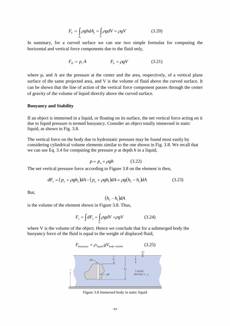
Buoyancy and Stability
If an object is immersed in a liquid, or floating on its surface, the net vertical force acting on it
due to liquid pressure is termed buoyancy. Consider an object totally immersed in static
liquid, as shown in Fig. 3.8.
The vertical force on the body due to hydrostatic pressure may be found most easily by
considering cylindrical volume elements similar to the one shown in Fig. 3.8. We recall that
we can use Eq. 3.4 for computing the pressure p at depth h in a liquid,
ghpp o (3.22)
The net vertical pressure force according to Figure 3.8 on the element is then,
dAhhgdAghpdAghpdF ooz 1212 (3.23)
But,
dAhh 12
is the volume of the element shown in Figure 3.8. Thus,
gVgdVdFFV
zz (3.24)
where V is the volume of the object. Hence we conclude that for a submerged body the
buoyancy force of the fluid is equal to the weight of displaced fluid,
volumebodyliquidbuoyancy gVF (3.25)
Figure 3.8 Immersed body in static liquid

- 44 -
The line of action of the buoyant force passes through the centre of volume of the displaced
body. For example the centre of mass is computed as if it had uniform density. The point
which buoyancyF acts is called the centre of buoyancy. Both liquids and gasses exert buoyancy
force on immersed bodies.
In the case of floating bodies, the body displaces its own weight in the fluid in which it floats,
thus,
volumebodydisplacedliquidbuoyancy gVF (3.26)
This relation reportedly was used by Archimedes in 220 B.C. to determine the gold content in
the crown of King Hiero II. Consequently, it is often called “Archimedes’ Principle.” In more
current technical applications, Eq. 3.25 is used to design displacement vessels, flotation gear,
and submersibles.
Figure 3.9Archimedes law of buoyancy.
Question 3-6
The gate shown is hinged at O and has constant width, w=5 m. The equation of the surface is
x=y2/a, where a=4 m. The depth of water to the right of the gate is D=4 m. Find the magnitude
of the force, Fa, applied as shown, required to maintain the gate in equilibrium if the weight of
the gate is neglected.
Solution 3-6
Given: Gate of constant width, w=5 m.
Equation of surface in xy plane is x=y2/a, where a=4 m.
Water stands at depth D=4 m to the right of the gate.
Force Fa is applied as shown, and weight of gate is to be neglected. (Note that
for simplicity we do not show the reactions at O.)

- 45 -
Find: Force Fa required maintaining the gate in equilibrium.
Solution:
We will take moments about point O after finding the magnitudes and locations of the
horizontal and vertical forces due to the water. The free body diagram (FBD) of the system is
shown above in part (a). Before proceeding we need to think about how we compute FV, the
vertical component of the fluid force—we have stated that it is equal (in magnitude and
location) to the weight of fluid directly above the curved surface. However, we have no fluid
directly above the gate, even though it is clear that the fluid does exert a vertical force! We
need to do a “thought experiment” in which we imagine having a system with water on both
sides of the gate (with null effect), minus a system with water directly above the gate (which
generates fluid forces). This logic is demonstrated above: the system FBD(a)=the null FBD(b)
- the fluid forces FBD(c). Thus the vertical and horizontal fluid forces on the system, FBD(a),
are equal and opposite to those on FBD(c). In summary, the magnitude and location of the
vertical fluid force FV are given by the weight and location of the centroid of the fluid
“above” the gate; the magnitude and location of the horizontal fluid force FH are given by the
magnitude and location of the force on an equivalent vertical flat plate.
Governing equations:
gVFV ApF cH c
xxc
Ay
Iyy 0OM
For FH, the centroid, area, and second moment of the equivalent vertical flat plate are,
respectively, yc=hc=D/2, A=Dw, and Ixx =wD3/12.
AghApF ccH
wD
gDwD
g22
2
mkg
Nsm
mm
m
kg
.5
2
4
sec81.9999
22
23
kNFH 392
and

- 46 -
c
xxc
Ay
Iyy
3
2
62)
2)((
12/
2
3 DDD
DwD
wDD
mmy 67.243
2
For FV, we need to compute the weight of water “above” the gate. To do this we define a
differential column of volume (D-y).w.dx and integrate
a
Da
Da
D
V dxaxDgwdxyDgwwdxyDggVF
222
0
21
00
)()()(
a
gwDa
a
D
a
DgwaxDxgw
aD
33
2
3
2 3
23
33
0
23
2
mkg
Ns
m
mm
m
m
kg
.4
1
3
45
sec81.9999
233
23
kNFV 261
The location x’ of this force is given by the location of the center of gravity of the water
“above” the gate. We recall from statics that this can be obtained by using the notion that the
moment of FV and the moment of the sum of the differential weights about the y axis must be
equal, so
a
Da
Da
D
V dxaxDxgwwdxyDxggdVxFx
222
0
23
00
)()(
2
5
25
5
2
5
0
25
2
105
2
25
2
2
2
a
gwDa
a
D
a
Dgwaxx
Dgw
aD
mm
m
a
D
Fa
gwDx
V
2.14
4
10
3
10
3
10
222
2
5
Now that we have determined the fluid forces, we can finally take moments about O (taking
care to use the appropriate signs), using the results calculated as above
0)( HVaO FyDFxlFM
HVa FyDFxl
F )(1
kNmkNm 39267.242612.15
1
kNFa 167

- 47 -
Question 3-7
Quantify the experiment performed by Archimedes to
identify the material content of King Hiero’s crown.
Assume you can measure the weight of the king’s crown in
air, Wa and the weight in water, Ww. Express the specific
gravity of the crown as a function of these measured
values.
Solution 3-7
Given: Experiment performed by Archimedes to identify the material content of King
Hiero’s crown. The crown was weighed in air and in water.
Find: Expression for the specific gravity of the crown as a function of the weights in
water and air.
Solution: We will apply the hydrostatic equations to this system
Governing equations:
db gVF Buoyant force is equal to weight of displaced fluid.
Assumptions: (1) static fluid and (2) incompressible fluid
Taking the free body diagram of the body as shown in the question
0 zF 0. bW FgMW
Ww is the weight of the crown in water;
dwbuoyW gVgMFgMW ..
However, in air;
gMWa .
Therefore the weight measured in water is
dwaW gVWW
So the volume is,
g
WWV
w
Wad
The density of the of the crown is w
wa
aw
wawa
w
d
crownWW
W
WW
Mg
WW
gM
V
M
Therefore, the specific gravity of the crown is;
wa
a
water
crown
WW
WSG

- 48 -
Question 3-8
A spherical body has a diameter of 1.5 m, weighs 8.5 kN,
and is anchored to the sea floor with a cable as is shown in
the figure. Calculate the tension of the cable when the body
is completely immersed, assume the specific weight of the
sea water is 10.1 kN/m2.
Solution 3-8
Given: The weight and the diameter of the sphere.
Find: Tension on the cable.
Solution: We will apply the hydrostatic equations and the buoyancy theorem.
The buoyancy force FB is shown in the free body diagram where W is the
weight of the body and T is the cable tension. For equilibrium, we have:
0 F WFT B
The buoyancy force is FB=γV. And the volume of the body is:
6
3dV
The cable tension then becomes;
kNNmNT 35.9)(105.86
5.1)/(101.10 3
333
Question 3-9
A rectangular sluice gate, 0.9m × 1.0m, is fitted at the base
of a reservoir wall with a pivot in the arrangement shown in
the Figure. The gate will open when the level of water in the
reservoir reaches a certain depth. Determine the weight, W,
that must be applied at the center of the gate, if a water level
of h = 2.0m will just cause the gate to open.
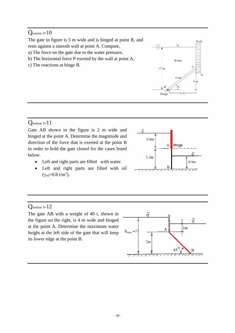
- 49 -
Question 3-10
The gate in figure is 5 m wide and is hinged at point B, and
rests against a smooth wall at point A. Compute,
a) The force on the gate due to the water pressure,
b) The horizontal force P exerted by the wall at point A,
c) The reactions at hinge B.
Question 3-11
Gate AB shown in the figure is 2 m wide and
hinged at the point A. Determine the magnitude and
direction of the force that is exerted at the point B
in order to hold the gate closed for the cases listed
below.
Left and right parts are filled with water.
Left and right parts are filled with oil
(γoil=0.8 t/m3).
Question 3-12
The gate AB with a weight of 40 t, shown in
the figure on the right, is 4 m wide and hinged
at the point A. Determine the maximum water
height at the left side of the gate that will keep
its lower edge at the point B.

- 50 -
Question 3-13
A rectangular plane area, immersed in water, is 1.5m by 1.8m, with the 1.5m side
horizontal and the 1.8m side vertical. Determine the magnitude of the force on one side and
the depth of its center of pressure if the top edge is
(a) in the water surface,
(b) 0.3m below the water surface,
(c) 30m below the water surface.
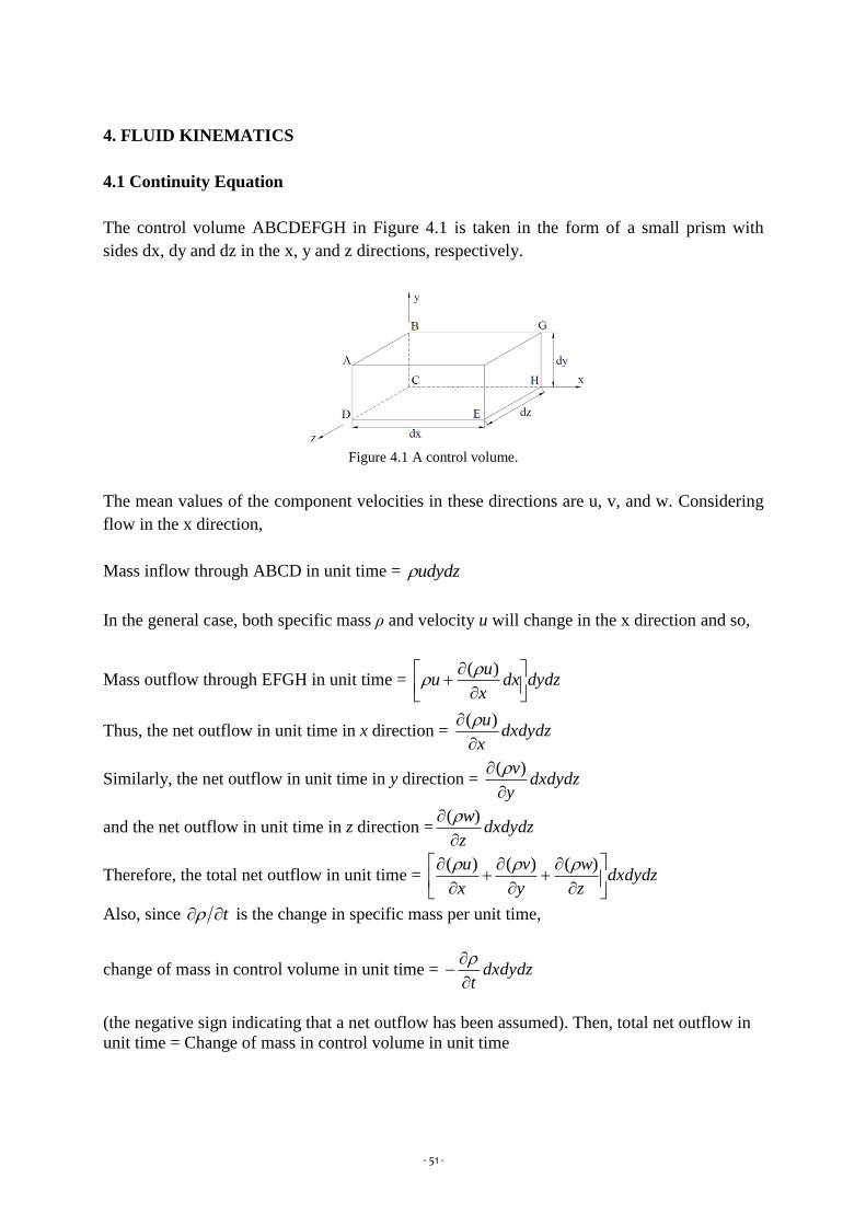
- 51 -
4. FLUID KINEMATICS
4.1 Continuity Equation
The control volume ABCDEFGH in Figure 4.1 is taken in the form of a small prism with
sides dx, dy and dz in the x, y and z directions, respectively.
Figure 4.1 A control volume.
The mean values of the component velocities in these directions are u, v, and w. Considering
flow in the x direction,
Mass inflow through ABCD in unit time = udydz
In the general case, both specific mass ρ and velocity u will change in the x direction and so,
Mass outflow through EFGH in unit time = dydzdxx
uu
)(
Thus, the net outflow in unit time in x direction = dxdydzx
u
)(
Similarly, the net outflow in unit time in y direction = dxdydzy
v
)(
and the net outflow in unit time in z direction = dxdydzz
w
)(
Therefore, the total net outflow in unit time = dxdydzz
w
y
v
x
u
)()()(
Also, since t is the change in specific mass per unit time,
change of mass in control volume in unit time = dxdydzt
(the negative sign indicating that a net outflow has been assumed). Then, total net outflow in
unit time = Change of mass in control volume in unit time

- 52 -
dxdydzz
w
y
v
x
u
)()()( = dxdydz
t
or
z
w
y
v
x
u
)()()( =
t
(4.1)
Equation (4.1) holds for every point in a fluid flow whether steady or unsteady, compressible
or incompressible. However, for incompressible flow, the density is constant and the equation
simplifies to
0
z
w
y
v
x
u (4.2)
For two-dimensional incompressible flow this will simplify still further to
0
y
v
x
u (4.3)
Question 4-1
The velocity distribution for the flow of an incompressible fluid is given by u = 3-x, v = 4+2y,
w = 2-z. Show that this satisfies the requirements of the continuity equation
Solution 4-1
For three-dimensional flow of an incompressible fluid, the continuity equation simplifies to
Equation (4.2);
0
z
w
y
v
x
u
In which,
1)3(
x
x
x
u
2)24(
y
y
y
v
1)2(
z
z
z
w
Therefore, 0121
z
w
y
v
x
u
which satisfies the requirement for continuity.
4.1 Stream Function for 2-D Flow
We already briefly discussed that streamlines were lines tangent to the velocity vectors in a

- 53 -
flow at an instant.
u
v
dx
dy
streamline
(4.4)
In this chapter we will develop a more formal definition of streamlines by introducing the
stream function ψ. This will allow us to represent two entities –the velocity components
u(x,y,t) and v(x,y,t) of a two-dimensional incompressible flow –with a single function ψ(x,y,t)
There are various ways to define the stream function. We will start with the two dimensional
version of the continuity equation for incompressible flow
0
y
v
x
u (4.5)
On the other hand, the velocity in x and y direction can be used to define the stream function
by,
yu
and
xv
(4.6)
Combining equation (4.5) and (4.6) results in:
022
xyyxy
v
x
u (4.7)
At the same time, by using the Equation (4.4) we can obtain an equation valid only along a
streamline,
0 vdxudy (4.8)
or using the definition of our stream function,
0
dy
ydx
x
(4.9)
On the other hand, at any instant in time t the variation in a function ψ(x,y,t) in space (x,y) is
given by,
ddyy
dxx
(4.10)
Comparing Equation (4.9) and (4.10) we see that along an instantaneous streamline, dψ=0; in
other words ψ is a constant along a streamline. Hence, we can specify individual streamlines
by their stream function values. The stream function is used to obtain the volume flow rate
between any two streamlines.
Consider the streamlines shown in Figure 4.2. We can compute the volume flow rate between
streamlines ψ1 and ψ2 by using line AB and BC.

- 54 -
Figure 4.2 Instantaneous streamlines in a two-dimensional flow.
Let us compute the flow rate by using line AB, and also by using line BC – they should be
same. For a unit depth, the flow rate across AB is
dyy
dyuQ
y
y
y
y
2
1
2
1
But along AB, x =constant, and from the Equation (4.7)
ddyy
, Therefore,
2
1
2
1
12
ddyy
Q
y
y
For a unit depth, the flow rate across BC is:
dxx
vdxQ
x
x
x
x
2
1
2
1
along BC, y =constant, and from the Equation (4.7)
ddxx
, Therefore,
1
2
2
1
12
ddxx
Q
x
x
Hence, whether we use line AB or line BC, we find that the volume flow rate (per unit depth)
between two streamlines is given by the difference between the two stream function values. If
the streamline through the origin is designated ψ=0, then the ψ value for any other streamline
represents the flow between the origin and that streamline. Note that because the volume flow
between any two streamlines is constant, the velocity will be relatively high wherever the
streamlines are close together, and relatively low wherever the streamlines are far apart.
Question 4-2
Given the velocity field for steady incompressible flow in a corner, AyjAxiV with A =
0.3 s-1, determine the stream function that will yield this velocity field. Plot and interpret the
streamline pattern in the first and second quadrants of the xy plane.

- 55 -
Solution 4-2
Given: velocity field, AyjAxiV with A = 0.3 s-1.
Find: The stream function and plot in first and second quadrants; interpret the results
Solution:
The flow is incompressible so the stream function satisfies Equation (4.6)
yAxu
yAx
dAxdy
)(1 xfAxy (1)
where f1(x) is an arbitrary value. The function f1(x) can be evaluated using the equation for v.
Thus,
xAyv
xAy
dAydx
)(2 xfAxy (2)
From Equations (1) and (2) it is clear that the f1(x) and f2(x) are constant and can be
represented as a constant c.
cAxy (3)
Lines of constant ψ represent streamlines in the flow field. The constant c may be chosen as
any convenient value for plotting purposes. The constant is chosen as “zero” in order that the
streamline through the origin be designated as ψ=ψ1=0. Then the value for any other
streamline represents the flow between the origin and that streamline. With c=0 and A=0.3s-1,
then,
xy3.0 (m3/s/m)

- 56 -
Separate plots of the streamlines in the first and second quadrants are presented below. Note
that in quadrant 1, u>0, so ψ values are positive. In quadrant 2, u<0, so ψ values are negative.
In the first quadrant, since u>0 and v<0, the flow is from left to right and down. The volume
flow rate between the streamline ψ=ψ1 through the origin and the streamline ψ=ψ2 is
3.01212 Q (m3/s/m)
In the second quadrant, since u<0 and v<0, the flow is from right to left and down. The
volume flow rate between streamlines ψ7 and ψ9 is,
6.07979 Q (m3/s/m)
The negative sign is consistent with flow having u<0.
4.3 Motion of a fluid particle
A typical finite fluid element, within which we have selected an infinitesimal particle of mass
dm and initial volume dx dy dz, and time t, and as it may appear after a time interval dt are
shown in Figure 4.3.
Figure 4.3 Finite fluid element and infinitesimal particle at times t and t+dt.
We can decompose the particle motion into four components:
Translation
Rotation
Linear deformation
Angular deformation
During the translation the particle moves from one point to another, and rotation may occur
about any or all of the x y and z axes. Linear deformation is the condition in which particle’s
sides stretch or contract and during the angular deformation the angles between the sides of
the particle changes. Figure 4.4 shows a typical xy plane motion decomposed into the four
components described above.

- 57 -
Figure 4.4 Pictorial representation of the components of fluid motion.
Basically, there are two types of motion: translation and rotation. The two may exist
independently or simultaneously, in which case they may be considered as one superimposed
on the other. If a solid body is represented by square, then pure translation or pure rotation
may be represented as shown in Fig. 4.4 (a) and (b), respectively. If we now consider the
square to represent a fluid element, it may be subjected to deformation. This can be either
linear or angular, as shown in Fig. 4.3 (c) and (d), respectively. The rotational movement can
be specified in mathematical terms. Fig.4.5 shows the rotation of a rectangular fluid element
in a two-dimensional flow.
Figure 4.5 Rotation of a rectangular fluid element in a two dimensional flow.
During the time interval Δt the element ABCD has moved relative to A to a new position,
which is indicated by the dotted lines. The average of the angular velocities of these two line
elements is defined as the rotation, w of the fluid element ABCD. Therefore,
y
u
x
vwww ADAB
2
1
2
1 (4.11)
The condition of irrotationality for a two-dimensional flow is satisfied when the rotation w is
everywhere zero, so that

- 58 -
0
y
u
x
v or
y
u
x
v
(4.12)
For a three-dimensional flow, the condition of irrotationality requires that the rotation about
each of three axes, which are parallel to x, y and z-axes must be zero. Therefore, the following
three equations must be satisfied:
y
u
x
v
(4.12a)
z
v
y
w
(4.12b)
x
w
z
u
(4.12c)
Question 4-3
The velocity components in a two-dimensional velocity field for an incompressible fluid are
expressed as
yxxy
u 23
23
3
23
2 xyxyv
Show that these functions represent a possible case of an irrotational flow.
Solution 4-3
The functions given satisfy the continuity equation
xyx
u22
and
22
xy
y
v
So that,
02222
xyxy
y
v
x
u
Therefore they represent a possible case of fluid flow. The rotation w of any fluid element in
the flow field is
y
u
x
vwww ADAB
2
1
2
1

- 59 -
y
yxyx
x
xyxy )3/2()3/2(
2
1 3232
0)()(2
1 2222 xyxy
4.4 Velocity potential functions
When the flow is irrotational, a mathematical function called the velocity potential function φ
may also be found to exist. A velocity potential function φ for a steady, irrotational flow in
the xy-plane is defined as a function of x and y, such that the partial derivative φ with respect
to displacement in any chosen direction is equal to the velocity in that direction.
Therefore, for the x and y directions,
xu
(4.13)
yv
(4.14)
These equations indicate that the velocity potential increases in the direction of flow. When
the velocity potential function φ is equated to a series of constants, equations for a family of
equipotential lines are the result.
The continuity equation
0
y
v
x
u
may be written in terms of φ by substitution Eqs. (4.13) and (4.14) into the Equ. (4.3), to yield
the Laplacian differential equation,
02
2
2
2
2
yx (4.15)
Thus all practical flows (which must conform to the continuity principle) must satisfy the
Laplacian equation in terms of φ.
For any flow pattern the velocity potential function φ is related to the stream function ψ by the
means of the two velocity components, u and v, at any point (x, y) in the Cartesian coordinate
system in the form of the two following equations:
yxu
xyv

- 60 -
Question 4-4
A stream function in a two-dimensional flow is ψ = 2xy. Show that the flow is irrotational
(potential) and determine the corresponding velocity potential function
Solution 4-4
The given stream function satisfies the condition of irrotationality, that is
2
2
2
2
2
1
2
1
yxy
u
x
vw
02)2(
2
12
2
2
2
y
xy
x
xy
which shows that the flow is irrotational. Therefore, a velocity potential function φ will exist
for this flow.
xy
xy
yxu 2
)2(
Therefore,
)(2 1
2 yfxxx
And also
yx
xy
xyv 2
)2(
From this equation
)(2 2
2 xfyyy
The velocity potential function can therefore be defined as
Cyx 22

- 61 -
Question 4-5
In a two-dimensional, incompressible flow the fluid velocity components are given by: u = x
– 4y and v = -y - 4x. Show that the flow satisfies the continuity equation and obtain the
expression for the stream function. If the flow is potential (irrotational) obtain also the
expression for the velocity potential.
Solution 4-5
For incompressible, two-dimensional flow, the continuity equation is
0
y
v
x
u
u=x-4y and v=-y-4x
1
x
u 1
y
v
Therefore, 1-1=0 and the flow satisfy the continuity equation.
In order to obtain the stream function we should write down
yxy
u 4
(a)
xyx
v 4
(b)
Therefore, from (a)
Cxfyyx )()4(
Cxfyxy )(2 2
But, if ψ1 = 0 at x = 0 and y = 0, which means that the reference streamline passes through the
origin, then C = 0 and
)(2 2 xfyxy (c)
To determine f (x), differentiate partially the above expression with respect to x and equate to
–v, equation (b):
xyx
xfy
x4
)(

- 62 -
224)( xxxxf
Substituting into (c)
22 22 yxyx
To check whether the flow is potential, there are two possible approaches:
since
0
y
u
x
v
but
u=x-4y and v=-y-4x
therefore,
044
y
u
x
v
and flow is potential.
Laplace equation must be satisfied
02
2
2
2
2
yx
22 22 yxyx
therefore
xyx
4
and yx
y4
42
2
x
and 4
2
2
y
Therefore, 4-4=0 and the flow is potential
yxx
u 4

- 63 -
Gyfxyx )()4(
But
00 at x=0 and y=0, so that G=0
Therefore,
)(42
2
yfyxx
Differentiating with respect to y and equation to v,
yxyfdy
dx
x
4)(4
yyfdy
d)( and
2)(
2yyf
So that
24
2
22 yyx
x
Question 4-6
A stream function is given by 323 yx
Determine the magnitude of velocity components at the point (3,1)
Solution 4-6
The x and y components of velocity are given by
x-component:
232
3)3(
yy
yx
yu
y-component:
xx
yx
xv 6
)3( 32

- 64 -
At the point (3,1)
3u and 18v
And the total velocity is the vector sum of the two components.
jiV 183
Question 4-7
The velocity components for a two-dimensional flow of an ideal and incompressible fluid are
given as u = −x and v = y .
Determine the stream function of the flow.
Determine if the flow is potential or not. If it is a potential flow, derive the velocity
potential function.
Compute the discharge per unit width through a line or a curve connecting the points
A(-1, 1) and B(-2, 3) in this flow field.
Question 4-8
The velocity components for a flow of an incompressible fluid are given by the following
equations:
u = k x (y + z); v = k y (x + z); w = −k z (x + y)− z2 .
• Determine the value of “k” in order to have a physically possible flow.
• Determine if the flow is steady or not (use the value of “k”, obtained in the first part).
• Determine if the flow is uniform or not (use the value of “k”, obtained in the first part).
• Determine if the flow is rotational or not (use the value of “k”, obtained in the first part). If it
is a rotational flow, compute the magnitude of rotations at a point A which has the following
coordinates: x=1, y=1, z=1.

- 65 -
5. BASIC EQUATIONS IN INTEGRAL FORM FOR A CONTROL VOLUME
We are now ready to study fluids in motion, so we have to decide how we are to examine a
flowing fluid. We can study a region of space as fluid flows through it, which is the control
volume approach. This is very often the method of choice, because it has widespread practical
application; for example, in aerodynamics we are usually interested in the lift and drag on a
wing (which we select as part of the control volume) rather than what happens to individual
fluid particles. The disadvantage of this approach is that the physical laws apply to matter and
not directly to regions of space, so we have to perform some math to convert physical laws
from their system formulation to a control volume formulation. We will examine the control
volume approach in the following section.
5.1 Basic Laws of the System
The basic laws we will apply are conservation of mass, Newton’s second law, and the first
law of thermodynamics. For converting these system equations to equivalent control volume
formulas, each of the laws are represented as a rate equation.
Conservation of Mass
For a system (by definition a fixed amount of matter, M, we have chosen), we have the simple
result that M=constant. However, as discussed above, we wish to express each physical law as
a rate equation, so we write
0
systemdt
dM (5.1)
where
)()( systemsystemMsystem ddmM (5.2)
Newton’s Second Law
For a system moving relative to an inertial reference frame, Newton’s second law states that
the sum of all external forces acting on the system is equal to the time rate of change of linear
momentum of the system,
systemdt
(5.3)
where the linear momentum of the system is given by

- 66 -
)()( systemsystemMsystem dVdmVP
(5.4)
The First Law of Thermodynamics
The first law of thermodynamics is a statement of conservation of energy for a system,
dEWQ (5.5)
The equation can be written in rate form as
systemdt
dEWQ
(5.6)
where the total energy of the system is given by
)()( systemsystemMsystem deedmE (5.7)
and
gzV
ue 2
2
(5.8)
In Eq. 5.6, Q (the rate of heat transfer) is positive when heat is added to the system from the
surroundings; W (the rate of work) is positive when work is done by the system on its
surroundings. In Eq. 5.8, u is the specific internal energy, V is the speed, and z the height
(relative to a convenient datum) of a particle of substance having mass dm.
5.2 Relation of System Derivatives to the Control Volume Formulation
We now have the three basic laws expressed as system rate equations. Our task in this section
is to develop a general expression for converting a system rate equation into an equivalent
control volume equation. Instead of converting the equations for rates of change of PM
, and
E one by one, we let all of them be represented by the symbol N . Hence N represents the
amount of mass, or momentum, or energy. Corresponding to this extensive property, we will
also need the intensive (i.e., per unit mass) property . Thus;
)()( systemsystemMsystem ddmN (5.9)
Comparing Eq. 5.9 with Eqs. 5.2, 5.4, and 5.7, we see that if:
,MN then 1
,PN
then V
,EN then e

- 67 -
How can we derive a control volume description from a system description of a fluid flow?
Before specifically answering this question, we can describe the derivation in general terms.
We imagine selecting an arbitrary piece of the flowing fluid at some time t0, as shown in Fig.
5.1a—we could imagine colouring this piece of fluid, say, blue.
Figure 5.1 System and control volume configuration.
This initial shape of the fluid system is chosen as our control volume, which is fixed in space
relative to coordinate’s xyz. After an infinitesimal time Δt the system will have moved
(probably changing shape as it does so) to a new location, as shown in Fig. 5.1b. The laws we
discussed above apply to this piece of fluid—for example, its mass will be constant. By
examining the geometry of the system/control volume pair at t=t0 and at t=t0+Δt, we will be
able to obtain control volume formulations of the basic laws.
From Fig. 5.1 we see that the system, which was entirely within the control volume at time t0,
is partially out of the control volume at time t0+Δt. In fact, three regions can be identified.
These are: regions I and II, which together make up the control volume, and region III, which,
with region II, is the location of the system at time t0+Δt.
Recall that our objective is to relate the rate of change of any arbitrary extensive property, N,
of the system to quantities associated with the control volume. From the definition of a
derivative, the rate of change of Nsystem is given by Reynolds Transport Theorem as
CSCV
system
AdVdtdt
dN . (5.10)
For the last term of the equation the scalar product of velocity vector and area vector need to
be considered. This concept of the sign of the scalar product is illustrated in Fig. 5.2 for (a)
the general case of an inlet or exit, (b) an exit velocity parallel to the surface normal, and (c)
an inlet velocity parallel to the surface normal. Cases (b) and (c) are obviously convenient
special cases of (a); the value of the cosine in case (a) automatically generates the correct sign
of either an inlet or an exit.

- 68 -
Figure 5.2 Evaluating the scalar product.
We need to be clear while evaluating the Reynolds transport theorem for control system. The
system is the matter that happens to be passing through the chosen control volume, at the
instant we chose. Let’s discuss the meaning of each term of the equation:
systemdt
dN
Is the rate of change of the system extensive property N , for example,
if PN
, we obtain the rate of change of momentum.
d
t CV
Is the rate of change of the amount of property N in the control
volume. The term dCV
computes the instantaneous value of N
in the control volume. For example, if PN
, then V
and
dVCV
computes the instantaneous amount of momentum in the
control volume.
CSAdV
.
Is the rate at which property N is exiting the surface of the control
volume. The term AdV
. computes the rate of mass transfer leaving
across control surface area element Ad
; multiplying by computes
the rate of flux of property N across the element; and integrating
therefore computes the net flux of N out of the control volume. For
example, if PN
, then V
and dVCV
computes the net flux
of momentum out of the control volume.
5.3 Conservation of Mass
The first physical principle to which we apply this conversion from a system to a control
volume description is the mass conservation principle: The mass of the system remains
constant,
0
systemdt
dM
where
)()( systemsystemMsystem ddmM
The system and control volume formulations are related by Eq. 5.10
CSCV
system
AdVdtdt
dN .

- 69 -
where
)()( systemsystemMsystem ddmN
to derive the control volume formulation of conservation of mass, we set
,MN and 1
with this substitution, we obtain
0.
CSCV
AdVdt
(5.11)
In Eq. 5.11 the first term represents the rate of change of mass within the control volume; the
second term represents the net rate of mass flux out through the control surface. Equation 5.11
indicates that the rate of change of mass in the control volume plus the net outflow is zero.
The mass conservation equation is also called the continuity equation. In common sense
terms, the rate of increase of mass in the control volume is due to the net inflow of mass:
Rate of increase of mass
in control volume
= Net influx of mass
CSCVAdVd
t
.
Once again, we note that in using the multiplication of vectors, care should be taken in
evaluating the scalar product AdV
. = cosVdA ; it could be positive, negative or even zero. It
is possible to simplify the continuity equation. Consider first the case of an incompressible
fluid, in which density remains constant. When density is constant, it is not a function of
space and time. Consequently, for incompressible fluids, the equation can be written as
0.
CSCV
AdVdt
The integral of d over the control volume is simply the volume of the control volume. Thus,
on dividing through by , we write
0.
CS
AdVt
For a non-deformable control volume of fixed size and shape the volume is constant. The
conservation of mass for incompressible flow through a fixed control volume becomes
0. CSAdV
a useful special case is when we have uniform velocity at each inlet and exit. In this case
above equation simplifies to
0. CSAdV
(5.12)
The final form of the continuity equation is the statement of conservation of mass for flow of
an incompressible fluid that may be steady or unsteady. The dimensions of integral form of
the continuity equation is L3/T. Therefore, the integral form of AdV
. over a section of the
control surface is commonly called the volume flow rate or volume rate of flow. Thus, for

- 70 -
incompressible flow, the volume flow rate into a fixed control volume must be equal to the
volume flow rate out of the control volume. The volume flow rate Q , through a section of a
control surface of area A, is given by;
AAdVQ
. (5.13)
The average velocity magnitude, V
, at a section is defined as
A
AdVAA
QV
.
1
Consider now the general case of steady, compressible flow through a fixed control volume.
Since the flow is steady, by definition, no fluid property varies with time in a steady flow.
Consequently, for steady flow, the statement of conservation of mass reduces to
0. CSAdV
(5.14)
A useful special case is when we have (or can approximate) uniform velocity at each inlet and
exit. In this case conservation of mass reduces to
0. CSAV
(5.15)
Thus, for steady flow, the mass flow rate into a control volume must be equal to the mass
flow rate out of the control volume.
Question 5-1
Consider the steady flow in a water pipe joint
shown in the diagram. The areas are: A1=0.2m2,
A2=0.2m2, and A3=0.15m2 In addition, fluid is lost
out of a hole at 4 , estimated at a rate of 0.1
m3/sec. The average speeds at sections 1 and 3 are
V1=5 m/sec and V3=12 m/sec respectively. Find
the velocity at section 2
Solution 5-1
Given: Steady flow of water through the device.
A1 = 0:2m2 A2 = 0:2m2 A3 = 0:15m2
V1 = 5m/s V3 = 12m/s ρ = 999 kg/m3
Volume flow rate at section 4 = 0.1 m3/s
Find: Velocity at section 2.
Solution:

- 71 -
Choose a fixed control volume as shown. Make an
assumption that the flow at section 2 is outwards,
and label the diagram accordingly (if this
assumption is incorrect our final result will tell us).
Governing equation: The general control volume equation is Eq. 5.11, but we can go
immediately to Eq. 5.15 because of assumptions (2) and (3) below,
0. CSAV
Assumptions: (1) Steady flow (given).
(2) Incompressible flow.
(3) Uniform properties at each section.
Hence (using Eq. 5.15) and remembering that density is constant Equation 5.14 reduces to
04332211 QAVAVAV
where Q4 is the flow rate out of the leak.
Let us examine the first three terms in Eq. 1 in light of the discussion of Fig. 5.2 and the
directions of the velocity vectors:
1111 AVAV
Sign of 11 AV
is negative at
surface 1
2222 AVAV
Sign of 22 AV
is positive at
surface 2
3333 AVAV
Sign of 33 AV
is positive at
surface 3

- 72 -
Using these results in Eq. 1,
04332211 QAVAVAV
02
433112
A
QAVAVV
2.0
1.0)15.012()2.05(2
V
5.42 V m/sec
Recall that V2 represents the magnitude of the velocity, which we assumed was outwards
from the control volume. The fact that V2 is negative means that in fact we have an inflow at
location 2 —our initial assumption was invalid.
Question 5-2
The fluid in direct contact with a stationary solid boundary has zero velocity; there is no slip
at the boundary. Thus the flow over a flat plate adheres to the plate surface and forms a
boundary layer, as depicted below. The flow ahead of the plate is uniform with velocity
iUV
; U 30 m/s. The velocity distribution within the boundary layer ( y0 ) along
cd is approximated as:
2
2
yy
U
u
The boundary-layer thickness at location d is δ=5 mm. The fluid is air with density ρ=1.24
kg/m3. Assuming the plate width perpendicular to the paper to be w=0.6 m, calculate the
mass flow rate across surface bc of control volume abcd.
Solution 5-2
Given: Steady, incompressible flow over a flat plate, ρ=1.24 kg/m3. Width of plate, w=0.6 m.
Velocity ahead of plate is uniform: iUV
; U 30 m/s.
At x=xd:
δ=5 mm
2
2
yy
U
u

- 73 -
Find: Mass flow rate across surface bc.
Solution: The fixed control volume is shown by the dashed lines in the question
Governing equation: The general control volume equation is Eq. 5.11, but we can go
immediately to Eq. 5.14 because of assumptions (1) below,
0. CSAdV
Assumptions: (1) Steady flow (given).
(2) Incompressible flow.
(3) Two dimensional flow, given properties are independent of z.
Assuming that there is no flow in the z direction, then
0....)()()()(
daAcdAbcAabAAdVAdVAdVAdV
Since there is no flow across the surface (da); 0.)(
daAAdV
Hence,
0...)()()(
cdAbcAabAAdVAdVAdV
Changing the subject of the formula will help to find the mass flow rate across the surface
(bc), bcm ;
)()()(
...cdAabAbcA
AdVAdVAdV
We need to evaluate the integrals on the right side of the equation. For depth w in the z
direction, we can obtain
yb
yaabAabAuwdyudAAdV
)()(.
00
Uwdyuwdy
UwUwy 0
AdV
. is negative
wdydA
Uu over area ab
yc
ydcdAcdAuwdyudAAdV
)()(.
0
2
02 dy
yywUuwdy
AdV
. is positive

- 74 -
3
11
30
2
2
32
wUyy
wU
3
2 wU
wdydA
Substituting into Equation 1, we obtain
33
2
wUwUwUmbc
0372.01000
56.03024.1
3
1bcm /sec.
The positive sign indicates flow out across the surface bc.
Question 5-3
A tank of 0.05 m3 volume contains air at 800 kPa (absolute)
and 15oC. At t=0, air begins escaping from the tank through a
valve with a flow area of 65 mm2. The air passing through the
valve has a speed of 300 m/s and a density of 6 kg/m3.
Determine the instantaneous rate of change of density in the
tank at t=0.
Solution 5-1
Given: A tank of 0.05 m3 volume contains air at 800 kPa (absolute) and 15oC. At t=0, air
escapes through a valve. Air leaves with speed V= 300 m/s and density ρ = 6 kg/m3 through
area 65 mm2.
Find: Rate of change of air density in the tank at t=0.
Solution: Choose a fixed control volume as shown.
Governing equation: 0.
CSCV
AdVdt
Assumptions: (1) Properties in the tank are uniform, but time-dependent.
(2) Uniform flow at section 1.
Since properties are assumed uniform in the tank at any instant, we can take density, ρ out
from within the volume integral of the first term,

- 75 -
0.
CSCV
CV AdVdt
Now CVd and hence
0.
CS
CV AdVt
The only place where mass crosses the boundary of the control volume is at surface 1. Hence,
1
..ACS
AdVAdV
and therefore
0.1
ACV AdV
t
At surface 1 the sign of AdV
. is positive and uniform, so 1111
. AVAdVA
Then,
0. 111
AV
tCV or 111 .AV
tCV
Since the volume, of the tank is not a function of time,
111 .AVt
and
111 .AV
t
At t=0,
26
2
3
2
3 1005.0
1653006
mm
m
mmm
s
m
m
kg
t
34.2
t
(kg/m3)/sec (the result shows that the density is decreasing)
5.3 Conservation of Momentum
Recall that Newton’s second law for a system moving relative to an inertial coordinate system
was given as
systemdt
Where the linear momentum of the system is given by
)()( systemsystemMsystem dVdmVP
and the resultant force, F
, includes all surface and body forces acting on the system,

- 76 -
BS FFF
The system and control volume formulations are related using Reynolds Transport Theorem
CSCV
system
AdVdtdt
dN .
To derive the control volume formulation of Newton’s second law, we set
,PN
then V
With this substitution, we obtain
CSCVsystem
AdVVdVtdt
Pd
.
Since the BS
system
FFFdt
Pd
The final equation can be achieved as:
CSCVBS AdVVdV
tFFF
. (5.17)
For the cases when we have uniform flow at each inlet and exit, we can use
CSCVBS AdVVdV
tFFF
. (5.18)
Equations 5.17 and 5.18 are our (nonaccelerating) control volume forms of Newton’s second
law. It states that the total force (due to surface and body forces) acting on the control volume
leads to a rate of change of momentum within the control volume (the volume integral) and/or
a net rate at which momentum is leaving the control volume through the control surface. We
must be a little careful in applying Eqs. 5.17 and 5.18. The first step will always be to
carefully choose a control volume and its control surface so that we can evaluate the volume
integral and the surface integral (or summation); each inlet and exit should be carefully
labelled, as should the external forces acting. In fluid mechanics the body force is usually
gravity, so
MgWgdF CVCV
B
(5.19)
Where g is the acceleration of gravity and CVW
is the instantaneous weight of the entire
control volume. In many applications the surface force is due to pressure,
AS ApdF
(5.20)
Note that we always compute pressure forces acting onto the control surface (recall that area
vector was chosen to be a vector pointing out of the control volume). It is worth stressing that
even at points on the surface that have an outflow, the pressure forces acts onto the control
volume.
Question 5-4
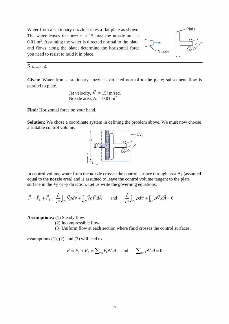
- 77 -
Water from a stationary nozzle strikes a flat plate as shown.
The water leaves the nozzle at 15 m/s; the nozzle area is
0.01 m2. Assuming the water is directed normal to the plate,
and flows along the plate, determine the horizontal force
you need to resist to hold it in place.
Solution 5-4
Given: Water from a stationary nozzle is directed normal to the plate; subsequent flow is
parallel to plate.
Jet velocity, V
= 15i m/sec.
Nozzle area, An = 0.01 m2
Find: Horizontal force on your hand.
Solution: We chose a coordinate system in defining the problem above. We must now choose
a suitable control volume.
In control volume water from the nozzle crosses the control surface through area A1 (assumed
equal to the nozzle area) and is assumed to leave the control volume tangent to the plate
surface in the +y or -y direction. Let us write the governing equations.
CSCVBS AdVVdV
tFFF
. and 0.
CSCV
AdVdt
Assumptions: (1) Steady flow.
(2) Incompressible flow.
(3) Uniform flow at each section where fluid crosses the control surfaces.
assumptions (1), (2), and (3) will lead to
CSBS AVVFFF
. and 0. CS
AV

- 78 -
The control volume has been selected so that the area of the
left surface is equal to the area of the right surface. Denote
this area by A. The control volume cuts through your hand.
We denote the components of the reaction force of your hand
on the control volume as Rx and Ry and assume both to be
positive. (The force of the control volume on your hand is
equal and opposite to Rx and Ry.)
Atmospheric pressure acts on all surfaces of the control
volume. Note that the pressure in a free jet is ambient, i.e., in
this case atmospheric. (The distributed force due to
atmospheric pressure has been shown on the vertical faces
only.)
The body force on the control volume is denoted as W. Since we are looking for the horizontal
force, we write the x component of the steady flow momentum equation
CSBxSx AVuFFF
.
There are no body forces in the x direction, so FBx = 0, and
CSSx AVuFF
.
To evaluate FSx , we must include all surface forces acting on the control volume
FSx= patmA
force due to atmospheric
pressure acts to right
(positive direction) on left
surface
- patmA
force due to atmospheric
pressure acts to left
(negative direction) on
right surface
+ Rx
force of your hand on
control volume (assumed
positive)
Consequently, xSx RF
and
1.. AVuAVuRFCSxSx
for top and bottom surfaces, 0u
111 AVuRF xSx
Since the angle between 1V
and 1A
is 180o
their scalar product will be (-)
mkg
sNm
s
m
m
kg
s
mRx
.
.01.01599915
22
3
kNRx 25.2 in which Rx acts opposite to positive direction assumed. Therefore, the
horizontal force acting on your hand is
kNRK xx 25.2

- 79 -
Question 5-5
Water flows steadily through the 90o reducing elbow shown
in the diagram. At the inlet to the elbow, the absolute
pressure is 220 kPa and the cross-sectional area is 0.01 m2.
At the outlet, the cross-sectional area is 0.0025 m2 and the
velocity is 16 m/s. The elbow discharges to the atmosphere.
Determine the force required to hold the elbow in place.
Solution 5-5
Given: Steady flow of water through 90o reducing elbow.
1P = 220 kPa (abs), A1 = 0.01 m2 2V
= -16j m/sec. A2 = 0.0025 m2
Find: Force required to hold the elbow in place.
Solution: We chose a coordinate system in defining the problem above. We must now choose
a suitable control volume.
Choose a fixed control volume as shown. Note that we have several surface force
computations: 1P on area A1 and atmP everywhere else. The exit at section 2 is to a free jet,
and so at ambient (i.e., atmospheric) pressure. We can use a simplification here: If we subtract
atmP from the entire surface (a null effect as far as forces are concerned) we can work in gage
pressures, as shown. Note that since the elbow is anchored to the supply line, in addition to
the reaction forces Rx and Ry (shown), there would also be a reaction moment (not shown).
Governing equation:
CSCVBS AdVVdV
tFFF
. (momentum equation)
0.
CSCV
AdVdt
(continuity equation)
Assumptions: (1) Steady flow (given).
(2) Incompressible flow.
(3) Uniform flow at each section.

- 80 -
(4) Atmospheric pressure, atmP =101 kPa (abs)
(5) Neglect weight of elbow and water in elbow
Once again (although we didn’t need to) we started with the most general form of the
governing equations. Writing the x component of the momentum equation results in
CSCVBxSx AdVudu
tFFF
.
where
0BxF
since there is no body force (weight) in x direction.
0
CV
dut
since the flow in the system is steady
Also the x- component of the velocity at section 2 does not exist,
Therefore;
1
..ACS
Sx AdVuAdVuF
1
11 .A
x AdVuRAP
1
11 .A
x AdVuAPR
Since the flow in the system is uniform than the integration part becomes summation of all the
forces:
11111 AVuAPRx
11111 AVuAPRx
Note that u1 is the x component of the velocity, so that u1=V1. To find V1, use the mass
conservation equation:
0...21
AACSAdVAdVAdV
02211 AVAV
and
401.0
0025.016
1
221
s
m
A
AVV m/sec.
We can now compute Rx
1
2
111 AVAPRx
mkg
Nsm
m
m
kgm
m
NRx
.01.0
sec1699901.01019.1
22
2
2
3
2
2
5
kNRx 35.1
Writing the y-component of the momentum equation gives

- 81 -
2
..ACS
BySy AdVvAdVvFFF
or
2
.A
Byy AdVvFR
222 .AVvFR Byy
Note that v2 is the y component of the velocity, so that v2=-V2 where V2, is the magnitude of
the exit velocity. Substituting known values:
222 .AVvFR Byy
222 AVvFR Byy
mkg
sNm
s
m
m
kgFR Byy
.
.0025.0)16(999
22
2
22
3
NFR Byy 639
Neglecting the weight of the system gives
NRy 639
Question 5-6
Water in an open channel is held in by a
sluice gate. Compare the horizontal force of
the water on the gate (a) when the gate is
closed and (b) when it is open (assuming
steady flow, as shown). Assume the flow at
sections 1 and 2 is incompressible and
uniform, and that (because the streamlines
are straight there) the pressure distributions
are hydrostatic.
Solution 5-6
Given: Flow under sluice gate. Width = w
Find: Horizontal force (per unit withd) on the closed and open gate

- 82 -
Solution: Choose a control volume as shown for the open gate. Note that it is much simpler to
work in gate pressures, as we learned in previous example.
The forces acting on the control volume include:
Force of gravity, W.
Friction force Ff.
Components Rx and Ry of reaction force from gate.
Hydrostatic pressure distribution on vertical surfaces.
Pressure distribution Pp(x) along bottom surface (not shown).
Apply the x component of the momentum equation.
Governing equation:
CSCVBxSx AdVudu
tFFF
.
0BxF
since there is no body force (weight) in x direction.
0
CV
dut
since the flow in the system is steady
Assumptions: (1) Steady flow.
(2) Incompressible flow (given).
(3) Uniform flow at each section.
(4) Ff negligible (neglect friction on channel bottom)
(5) Hydrostatic pressure distributions at section 1 and 2 are given
(6) 0BxF
Then,
22211121 wDVuwDVuRFFFF xRRSx
The surface forces acting on the CV are due to the pressure distributions and the unknown
force Rx. From assumption (6), we can integrate the gage pressure distributions on each side
to compute the hydrostatic forces FR1 and FR2 ,
2
1
1
0
21
0
1
0
112
1
2gwD
ygwgydywdAPF
DDD
R

- 83 -
where y is measured downward from the free surface of location 1 , and
2
2
2
0
22
0
2
0
222
1
2gwD
ygwgydywdAPF
DDD
R
where y is measured downward from the free surface of location 2. (Note that we could have
used the hydrostatic force equation, directly to obtain these forces.)
Evaluating FSx gives
2
2
2
12
DDgw
RF xSX
Substituting into the momentum equation, with u1=V1 and u2=V2, gives
2
2
21
2
1
2
2
2
12
wDVwDVDDgw
Rx
or
2
2
2
11
2
12
2
22
DDgw
DVDVwRx
The second term on the right is the net hydrostatic force on the gate; the first term “corrects”
this (and leads to a smaller net force) for the case when the gate is open. What is the nature of
this “correction”? The pressure in the fluid far away from the gate in either direction is indeed
hydrostatic, but consider the flow close to the gate: Because we have significant velocity
variations here (in magnitude and direction), the pressure distributions deviate significantly
from hydrostatic—for example, as the fluid accelerates under the gate there will be a
significant pressure drop on the lower left side of the gate. Deriving this pressure field would
be a difficult task, but by careful choice of our CV we have avoided having to do so!
We can now compute the horizontal force per unit width,
2
2
2
11
2
12
2
22
DDg
DVDVw
Rx
mkg
sNm
s
m
m
kg
w
Rx
.
.31429.07999
2
2
222
3
mkg
sNm
s
m
m
kg
w
Rx
.
.429.0381.9999
2
1 2222
23
mkNmkNw
Rx /2.43/0.18
mkNw
Rx /2.25
Rx is the external force acting on the control volume, applied to the CV by the gate. Therefore,
the force of the water on the gate is Kx, where Kx=-Rx. Thus,
mkNw
R
w
K xx /2.25
This force can be compared to the force on the closed gate of 44.1 kN (obtained from the
second term on the right in the equation above, evaluated with D2 set to zero because for the

- 84 -
closed gate there is no fluid on the right of the gate)—the force on the open gate is
significantly less as the water accelerates out under the gate.
5.3 Conservation of Energy
The first law of thermodynamics is a statement of conservation of energy. Recall that
the system formulation of the first law was
systemdt
dEWQ
Where the total energy of the system is given by
)()( systemsystemMsystem deedmE
and
gzV
ue 2
2
Q is the rate of heat transfer and is positive when heat is added to the system from the
surroundings. The rate of work, W , is positive when work is done by the system on its
surroundings. To derive the control volume formulation of the first law of thermodynamics,
we can set
EN and e
In which we obtain
CSCV
system
AdVedetdt
dE . (5.21)
Which can be simplified into
CSCVAdVede
tWQ
.
Integrating the above equation under the steady flow conditions results in the following
equation
gzVdP
2
2
constant (along a streamline) (5.22)
In the case of incompressible flow, the first terms also becomes an exact differential, and its
integration gives:
Steady, incompressible flow: gzVP
2
2
constant (along a streamline)
This is the famous Bernoulli Equation, which is commonly used in fluid mechanics for
steady, incompressible flow along a streamline in inviscid regions of flow. The value of the

- 85 -
constant can be evaluated at any point on the streamline where the pressure, density, velocity
and elevation are known. The Bernoulli equation can also be written between any two points
on the same streamline as
2
2
221
2
11
22gz
VPgz
VP
(5.23)
The Bernoulli equation is obtained from the conservation of momentum for a fluid particle
moving along a streamline. We recognize V2/2 as kinetic energy gz as potential energy and
P/ρ as flow energy, all per unit mass. Therefore, the Bernoulli equation can be viewed as an
expression of mechanical energy balance and can be stated as follows:
The sum of the kinetic, potential and flow energies of a fluid particle is constant along a
streamline during steady flow when the compressibility and frictional effects are negligible.
The kinetic, potential, and flow energies are the mechanical forms of energy. The Bernoulli
equation can be viewed as the “conservation of mechanical energy principle.” This is
equivalent to the general conservation of energy principle for systems that do not involve any
consversiton of mechanical energy and thermal energy to each other, and thus the mechanical
energy and thermal energy are conserved separately. The Bernoulli equation states that during
steady, incompressible flow with negligible friction, the various forms of mechanical energy
are converted to each other, but their sum remains constant. In other words, there is no
dissipation of mechanical energy during such flows since there is no friction that converts
mechanical energy to sensible thermal energy. Recall that energy is transferred to a system as
work when a force is applied to a stytem through a distance. In the light of Newton’s second
law of motion, the Bernoulli equation is commonly used in practice since a variety of
practical fluid flow problems can be analysed to reasonable accuracy with it. This is because
many flows of practical engineering interest are steady (or at least steady in the mean),
compressibility effects are relatively small, and net frictional forces are negligible in regions
of interest in the flow.
Static, Dynamic and Stagnation Pressures
The Bernoulli equation states that the sum of the flow kinetic, and potential energies of a fluid
particle along a streamline is constant. Therefore, the kinetic and potential energies of the
fluid can be converted to flow energy (and vice versa) during flow, causing the pressure to
change. This phenomenon can be made more visible by multiplying the Bernoulli equation by
the density ρ.
gzV
P 2
2
constant (along a streamline) (5.24)
Each term here represents pressure units, and thus each term represents some kind of pressure.
P is the static pressure (it does not incorporate any dynamic effects); it represents the actual
thermodynamic pressure of the fluid.

- 86 -
2
2V is the dynamic pressure, it represents the pressure rise when the fluid in motion is
brought to a stop.
gz is the hydrostatic pressure, which is not a pressure in a real sense since its value depends
on the reference level selected; it accounts for the elevation effects.
The sum of the static, dynamic and hydrostatic pressure is called the total pressure. Therefore,
the Bernoulli equation states that the total pressure along a streamline is constant. The sum of
the static and dynamic pressures is called the stagnation pressure, and it is expressed as:
2
2VPPstag (5.25)
The stagnation pressure represents the pressure at a point where the fluid is brought to a
complete stop isentropically. The static, dynamic, and stagnation pressures are shown in the
following figure. When static and stagnation pressures are measured at a specific location, the
fluid velocity at that location can be calculated from
PPV
stag
2 (5.26)

- 87 -
Question 5-7
Water is flowing from a hose attached to a water main at 400kPa
gage. A child places his thumb to cover most of the hose outlet,
causing a thin jet of high speed water to emerge. If the hose is held
upward, what is the maximum height that the jet could achieve?
Solution 5-7
Given: Flow pressure at hose is 400kPa and the density of water is 1000kg/m3
Find: The maximum height that the jet could achieve.
Assumptions: (1) Steady flow.
(2) Incompressible and irrotational flow.
(3) The friction between the water and air is negligible.
Then,
Solution: This problem involves the conversion of flow, kinetic and potential energies to each
other without involving any pumps, turbines and wasteful components with large frictional
losses, and thus it is suitable for the use of the Bernoulli equation. The water height will be
maximum under the stated assumptions. The velocity inside the hose is relatively low (V1=0)
and we take the hose outlet as the reference level (z1=0). At the top of the water trajectory
V2=0 and atmospheric pressure pertains. Then the Bernoulli equation simplifies to
2
2
221
2
11
22gz
VPgz
VP
022
2
2
2
1 VV
and 01 z atmPP 2
Therefore

- 88 -
21 gz
PP atm
Solving for z2 substituting,
g
P
g
Pz atm
1
2 = mN
mkg
kPa
mN
smmkg
kPakPa8.40
1
sec/1
1
/1000
81.91000
0400 22
23
Therefore, the water jet can rise as high as 40.8 m into the sky in this case. The result obtained
by the Bernoulli equation represents the upper limit and should be interpreted accordingly. It
tells us that the water cannot possibly rise more than 40.8m, and, in all likelihood, the rise will
be much less than 40.8 m due to irreversible losses that we neglected.
Question 5-8
A large tank open to the atmosphere is filled with water to a
height of 5 m from the outlet tap. A tap near the bottom of
the tank is now opened, and water flows out from the
smooth and rounded outlet. Determine the water velocity at
the outlet.
Solution 5-8
Given: The height of water is 5 meters.
Find: The exit velocity of water from the tank is to be determined.
Assumptions: (1) The water drains slowly enough that the flow can be approximated as
steady.
(2) Incompressible and irrotational flow.
Then,
Solution: This problem involves the conversion of flow, kinetic and potential energies to each
other without involving any pumps, turbines and wasteful components with large frictional
losses, and thus it is suitable for the use of the Bernoulli equation. We take point 1 to be at the
free surface of water so that atmPP 1 (open to the atmosphere), V1=0 (the tank is large
relative to the outlet), and z1=5 meters and z2= 0 meter. (We take the reference level at the
centre of the outlet.) Also, atmPP 2 (water discharges into the atmosphere). Then the
Bernoulli equation simplifies to

- 89 -
2
2
221
2
11
22gz
VPgz
VP
02
2
1 V
and 02 z atmPPP 12
Therefore
2
2
21
Vgz
Solving for V2 substituting,
sec/9.9581.922 12 mgzV
The relation gzV 2 is called the Toricelli Equation. Therefore, the water leaves the tank
with an initial velocity of 9.9 m/sec.
Question 5-9
A piezometer and a Pitot tube are tapped into a horizontal
water pipe, as shown in the figure to measure static and
stagnation (static and dynamic) pressures. For the
indicated water column heights, determine the velocity at
the centre of the pipe.
Solution 5-9
Given: The height of water at different levels.
Find: Find the velocity at the centre of the pipe.
Assumptions: (1) The flow is steady and incompressible
(2) Points 1 and 2 are close enough together that the energy loss between these
two points is negligible.
Solution: We take points 1 and 2 along the centreline of the pipe, with point 1 directly under
the piezometer and point 2 at the tip of the Pitot tube. This is a steady flow with straight and
parallel streamlines, and the gage pressure at points 1 and 2 can be expresses as
211 hhgP
3212 hhhgP
Noting that point 2 is a stagnation point and thus V2=0 and z1=z2, the application of the
Bernoulli equation between points 1 and 2 gives

- 90 -
2
2
221
2
11
22gz
VPgz
VP
which reduces into
g
PP
g
V
12
2
1
2
Substituting the P1 and P2 expressions gives
3
2132112
2
1
2h
g
hhghhhg
g
PP
g
V
Solving for V1 and substituting
sec/53.112.081.922 31 mgzV
Note that to determine the flow velocity, all we need is to measure the height of the excess
fluid column in the Pitot tube.
Question 5-10
A university laboratory that generates 15 m3/s of air flow at design condition wishes to
build a wind tunnel with variable speeds. It is proposed to build the tunnel with a sequence
of three circular test sections: section 1 will have a diameter of 1.5 m, section 2 a diameter
of 1 m, and section 3 a diameter such that the average speed is 75 m/s.
(a) What will be the speeds in sections 1 and 2?
(b) What must the diameter of section 3 be to attain the desired speed at design
condition?
Question 5-11
Consider steady, incompressible flow through
the device shown. Determine the magnitude and
direction of the volume flow rate through port 3.

- 91 -
Question 5-12
Water flows steadily through a pipe of length L and
radius R=75 mm. Calculate the uniform inlet velocity,
U, if the velocity distribution across the outlet is given
by
and umax=3 m/s.
Question 5-13
Water enters a two-dimensional, square channel of
constant width, h=75.5 mm, with uniform velocity, U.
The channel makes a 90o bend that distorts the flow to
produce the linear velocity profile shown at the exit, with
vmax=2vmin. Evaluate vmin, if U=7.5 m/s.
Question 5-14
Water flows steadily past a porous flat
plate. Constant suction is applied along the
porous section. The velocity profile at
section cd is
Evaluate the mass flow rate across section
bc.
Question 5-15
A 30o reducing elbow is shown. The fluid
is water. Evaluate the components of force
that must be provided by the adjacent
pipes to keep the elbow from moving.

- 92 -
Question 5-16
Find the force required to hold the plug in place at the
exit of the water pipe. The flow rate is 1.5 m3/s, and the
upstream pressure is 3.5 MPa.
Question 5-17
A gate is 1 m wide and 1.2 m tall and hinged at the
bottom. On one side the gate holds back a 1-m-deep body
of water. On the other side, a 5-cm diameter water jet hits
the gate at a height of 1 m. What jet speed V is required
to hold the gate vertical? What will the required speed be
if the body of water is lowered to 0.5 m? What will the
required speed be if the water level is lowered to 0.25 m?
Question 5-18
Water enters a wide, flat channel of height 2h with a
uniform velocity of 2.5 m/s. At the channel outlet the
velocity distribution is given by the equation given at right
where y is measured from the centerline of the channel.
(a)Determine the exit centerline velocity, umax. (b) Ratio of
the x-direction momentum flux at the channel outlet to that
at the inlet
Question 5-19
Water flows steadily through the nozzle shown,
discharging to atmosphere. Calculate the
horizontal component of force in the flanged
joint. Indicate whether the joint is in tension or
compression.

- 93 -
Question 5-20
A reducer in a piping system is shown. The
internal volume of the reducer is 0.2 m3 and its
mass is 25 kg. Evaluate the total force that must
be provided by the surrounding pipes to support
the reducer. The fluid is gasoline. The specific
gravity of gasoline is 0.72.
Question 5-21
The inner diameter of a nozzle, which is attached to an 8 cm diameter garden hose, is given as 3
cm.
a. Compute the energy at the end section of the nozzle, i.e. at the point where the water leaves the
system, for a given discharge of 50 l/s.
b. Compute the forces acting on the nozzle for both of
the following cases:
• The system is running and its discharge is equal to
50 l/s.
• The system is not running and the water is at rest in
the garden hose.
Question 5-22
The discharge of water through a 140º bend, shown in
Figure, is 30 litres/s. The bend is lying in the horizontal
plane and the diameters at the entrance and exit are
200mm and 100mm respectively. The pressure measured
at the entrance is 100 kN/m2, what is the magnitude and
direction of the force exerted by the water on the bend?

- 94 -
Question 5-23
The velocity of the flow in the pipe shown in the figure is
measured as 3 m/s at the section “A”. Compute the power
transmitted to the turbine propeller (mounted at the section
“C”) by taking into consideration the relative pressure values
at the sections “A” and “B” of the pipe, given as 10 N/cm²
and -0.1 N/cm², respectively.
Question 5-24
A venturimeter is placed vertically as shown in
the figure. Compute the discharge of water
passing through the system by neglecting
energy losses and by considering the
indications of the manometer. (γmercury=136
kN/m³).

- 95 -
6. DIMENSIONAL ANALYSIS
Fluid mechanics is more heavily involved with experimental testing than other disciplines
because the analytical tools currently available to solve the momentum and energy equations
are not capable of providing accurate results. This is particularly evident in turbulent,
separating flows. The solutions obtained by utilizing techniques from computational fluid
dynamics with the largest computers available yield only fair approximations for turbulent
flow problems—hence the need for experimental evaluation and verification. For analyzing
model studies and for correlating the results of experimental research, it is essential that
researchers employ dimensionless groups. To appreciate the advantages of using
dimensionless groups, consider the flow of water through the unusual orifice illustrated in
Figure 6.1.
Figure 6.1 Flow through inverted flow nozzle
Because of size and expense it is not always feasible to carry out tests on a full-scale
prototype. Thus engineers will test a subscale model and measure the pressure drop across the
model. The test procedure may involve testing several orifices, each with a different throat
diameter d0. For purposes of discussion, assume that three nozzles are to be tested. The
Bernoulli equation suggests that the pressure drop will depend on flow velocity and fluid
density. It may also depend on the fluid viscosity. The test program may be carried out with a
range of velocities and possibly with fluids of different density (and viscosity). The pressure
drop, P1-P2, is a function of the velocity V1, density ρ, and diameter d0. By carrying out
numerous measurements at different values of V1 and ρ for the three different nozzles, the
data could be plotted as shown in Figure 6.2 for tests using water. In addition, further tests
could be planned with different fluids at considerably more expense.
Figure 6.2 Relations for pressure, velocity, and diameter using dimensional variables and dimensionless groups.
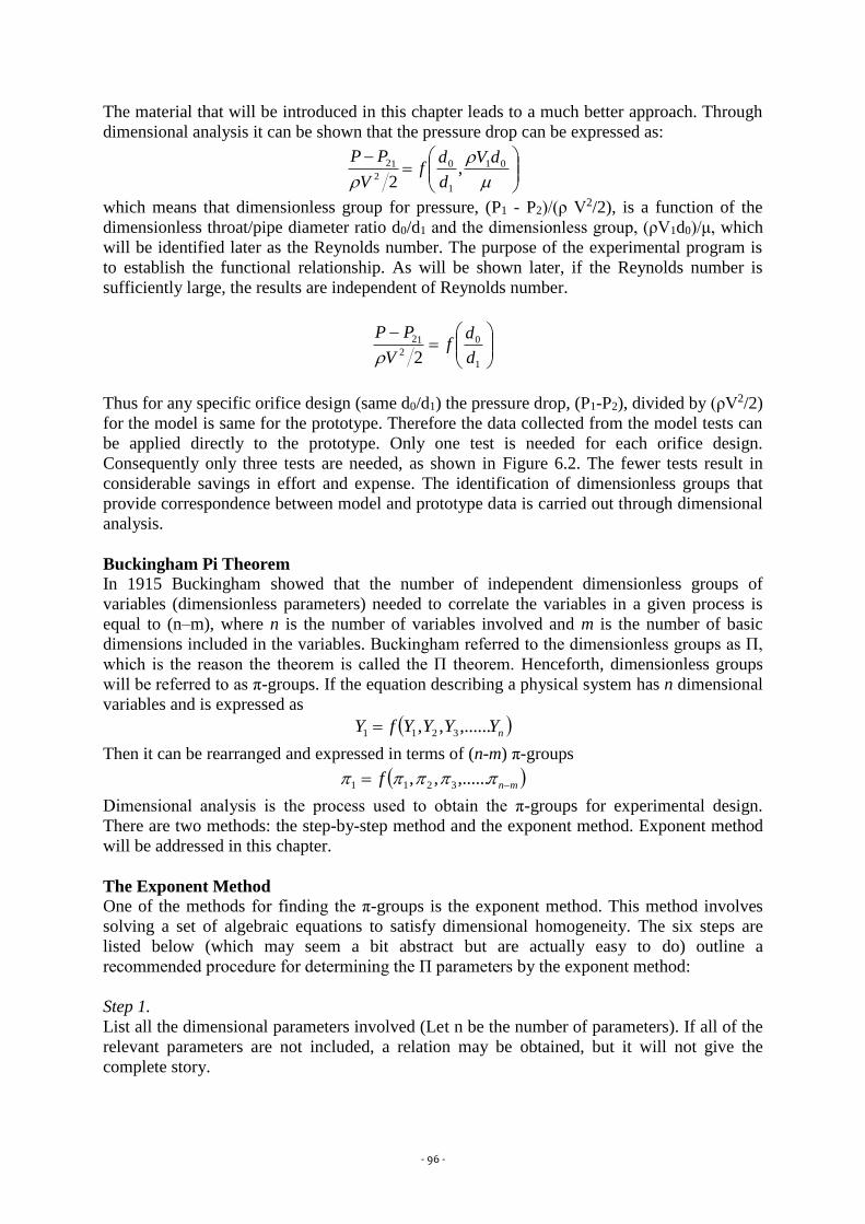
- 96 -
The material that will be introduced in this chapter leads to a much better approach. Through
dimensional analysis it can be shown that the pressure drop can be expressed as:
01
1
0
2
12 ,2
dV
d
df
V
PP
which means that dimensionless group for pressure, (P1 - P2)/(ρ V2/2), is a function of the
dimensionless throat/pipe diameter ratio d0/d1 and the dimensionless group, (ρV1d0)/μ, which
will be identified later as the Reynolds number. The purpose of the experimental program is
to establish the functional relationship. As will be shown later, if the Reynolds number is
sufficiently large, the results are independent of Reynolds number.
1
0
2
12
2 d
df
V
PP
Thus for any specific orifice design (same d0/d1) the pressure drop, (P1-P2), divided by (ρV2/2)
for the model is same for the prototype. Therefore the data collected from the model tests can
be applied directly to the prototype. Only one test is needed for each orifice design.
Consequently only three tests are needed, as shown in Figure 6.2. The fewer tests result in
considerable savings in effort and expense. The identification of dimensionless groups that
provide correspondence between model and prototype data is carried out through dimensional
analysis.
Buckingham Pi Theorem
In 1915 Buckingham showed that the number of independent dimensionless groups of
variables (dimensionless parameters) needed to correlate the variables in a given process is
equal to (n–m), where n is the number of variables involved and m is the number of basic
dimensions included in the variables. Buckingham referred to the dimensionless groups as Π,
which is the reason the theorem is called the Π theorem. Henceforth, dimensionless groups
will be referred to as π-groups. If the equation describing a physical system has n dimensional
variables and is expressed as
nYYYYfY ,......,, 3211
Then it can be rearranged and expressed in terms of (n-m) π-groups
mnf ,......,, 3211
Dimensional analysis is the process used to obtain the π-groups for experimental design.
There are two methods: the step-by-step method and the exponent method. Exponent method
will be addressed in this chapter.
The Exponent Method
One of the methods for finding the π-groups is the exponent method. This method involves
solving a set of algebraic equations to satisfy dimensional homogeneity. The six steps are
listed below (which may seem a bit abstract but are actually easy to do) outline a
recommended procedure for determining the Π parameters by the exponent method:
Step 1.
List all the dimensional parameters involved (Let n be the number of parameters). If all of the
relevant parameters are not included, a relation may be obtained, but it will not give the
complete story.

- 97 -
Step 2.
Select a set of fundamental (primary) dimensions, e.g., MLt or FLt. (Note that for heat
transfer problems you may also need T for temperature, and in electrical systems, q for
charge.)
Step 3.
List the dimensions of all parameters in terms of primary dimensions.
Step 4.
Select a set of r dimensional parameters that includes all the primary dimensions. These
parameters will all be combined with each of the remaining parameters, one of those at a time,
and so will be called repeating parameters. No repeating parameter should have dimensions
that are a power of the dimensions of another repeating parameter; for example, do not
include both an area (L2) and a second moment of area (L4) as repeating parameters. The
repeating parameters chosen may appear in all the dimensionless groups obtained;
consequently, do not include the dependent parameter among those selected in this step.
Step 5.
Set up dimensional equations, combining the parameters selected in Step 4 with each of the
other parameters in turn, to form dimensionless groups (There will be n-m equations). Solve
the dimensional equations to obtain the n-m dimensionless groups.
Step 6.
Check to see that each group obtained is dimensionless. If mass was initially selected as a
primary dimension, it is wise to check the groups using force as a primary dimension, or vice
versa. The functional relationship among the Π parameters must be determined
experimentally. The detailed procedure for determining the dimensionless Π parameters is
illustrated in Examples 6.1 and 6.2.
Question 6-1
The drag force, F, on a smooth sphere depends on the relative speed, V, the sphere
diameter, D, the fluid density, ρ, and the fluid viscosity, μ. Obtain a set of dimensionless
groups that can be used to correlate experimental data.
Solution 6-1
Given: ,,, DVfF for a smooth sphere.
Find: An appropriate set of dimensionless groups.
Solution: Follow the steps mentioned before
Step 1:
,,,, DVF n=5 dimensionless parameters
Step 2:
Select primary dimensions M,L, and T

- 98 -
Step 3:
F V D
2T
ML
3L
M
T
L L
LT
M
r=3 primary dimensions
Step 4:
Select repeating parameters while considering that combination of three repeating variables
should have at least each of these main primary dimensions, (MLT).
,V , D
3L
M
T
LL =
L
M
T
1 which possesses at least one L, one T and one M.
Step 5:
There are 5 dimensionless parameters and 3 of them are used as repeating variables.
Therefore, the number of resulting Π parameters will be 5-3=2.
FDV cba1 and 000
23TLM
T
MLL
T
L
L
M c
ba
cba DV 2 and 000
3TLM
LT
ML
T
L
L
M c
ba
Equating the exponents of M, L, and T of the first Π parameter will give:
:M 01a 1a
:L 013 cba 2c Therefore, 221
DV
F
:T 02 b 2b
Similarly for the second Π parameter
:M 01a 1a
:L 013 cba 1c Therefore, VD
2
:T 01b 1b
Step 6:
Check using F, L, T dimensions:
221DV
F
and 1
12
2
2
4
LL
T
FT
LF

- 99 -
VD
2 and 1
12
4
2
LL
T
FT
L
L
FT
The functional relationship is 21 f or,
VDf
DV
F
22
As noted before. The form of the function, f, must be determined experimentally
Question 6-2
The pressure drop, Δp, for steady, incompressible viscous flow through a straight
horizontal pipe depends on the pipe length, l, the average velocity, V, the fluid viscosity,
μ, the pipe diameter, D, the fluid density, ρ, and the average “roughness” height, e.
Determine a set of dimensionless groups that can be used to correlate data.
Solution 6-2
Given: elDVfP ,,,,, for a flow in a circular pipe.
Find: An appropriate set of dimensionless groups.
Solution: Follow the steps mentioned before
Step 1:
elDVP ,,,,,, n=7 dimensionless parameters
Step 2:
Select primary dimensions M,L, and T
Step 3:
P V D l e
2LT
M
3L
M
T
L L
LT
M L L
r=3 primary dimensions
Step 4:
Select repeating parameters while considering that combination of three repeating variables
should have at least each of these main primary dimensions, (MLT).
,V , D
3L
M
T
LL =
L
M
T
1 which possesses at least one L, one T and one M.

- 100 -
Step 5:
There are 7 dimensionless parameters and 3 of them are used as repeating variables.
Therefore, the number of resulting Π parameters will be 7-3=4.
PDV cba 1 and 000
23TLM
LT
ML
T
L
L
M c
ba
cba DV 2 and 000
3TLM
LT
ML
T
L
L
M c
ba
lDV cba3 and 000
3TLMLL
T
L
L
M c
ba
eDV cba4 and 000
3TLMLL
T
L
L
M c
ba
Equating the exponents of M, L, and T of Π1 :
:M 01a 1a
:L 013 cba 0c Therefore, 21
V
P
:T 02 b 2b
Similarly for the Π2 parameter
:M 01a 1a
:L 013 cba 1c Therefore, VD
2
:T 01b 1b
Similarly for the Π3 parameter
:M 0a 0a
:L 013 cba 1c Therefore, D
l 3
:T 0 b 0b
Similarly for the Π4 parameter
:M 0a 0a
:L 013 cba 1c Therefore, D
e 4
:T 0 b 0b

- 101 -
Step 6:
Check using F, L, T dimensions:
21V
P
and 1
2
2
4
2
L
T
FT
L
L
F
VD
2 and 1
12
4
2
LL
T
FT
L
L
FT
D
l 3 and 1
L
L
D
e 4 and 1
L
L
The functional relationship is 4321 ,, f or,
D
e
D
l
VDf
V
P,,
2
All the foregoing procedures deal with straightforward situations. However, some problems
do occur. In order to apply dimensional analysis one must first decide which variables are
significant. If the problem is not sufficiently well understood to make a good choice of the
significant variables, dimensional analysis seldom provides clarification. How does one know
if a variable is significant for a given problem? Probably the truest answer is by experience.
After working in the field of fluid mechanics for several years, one develops a feel for the
significance of variables to certain kinds of applications.
Common Pi-groups
The most common π-groups can be found by applying dimensional analysis to all the
variables that might be significant in a general flow situation, Variables that have significance
in a general flow field are the velocity V, the density ρ, the viscosity μ, and the acceleration
due to gravity g. In addition, if fluid compressibility were likely, then the bulk modulus of
elasticity, Ev, should be included. If there is a liquid-gas interface, the surface tension effects
may also be significant. Finally the flow field will be affected by a general length, l, such as
the width of a building or the diameter of a pipe. These variables will be regarded as the
independent variables. The primary dimensions of the significant independent variables are
vE V l g
2LT
M
3L
M
T
L
2T
M
LT
M L
2T
L
There are several other independent variables that could be identified for thermal effects, such
as temperature, specific heat, and thermal conductivity. Inclusion of these variables is beyond
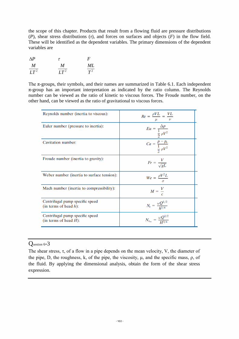
- 102 -
the scope of this chapter. Products that result from a flowing fluid are pressure distributions
(P), shear stress distributions (τ), and forces on surfaces and objects (F) in the flow field.
These will be identified as the dependent variables. The primary dimensions of the dependent
variables are
P F
2LT
M
2LT
M
2T
ML
The π-groups, their symbols, and their names are summarized in Table 6.1. Each independent
π-group has an important interpretation as indicated by the ratio column. The Reynolds
number can be viewed as the ratio of kinetic to viscous forces. The Froude number, on the
other hand, can be viewed as the ratio of gravitational to viscous forces.
Question 6-3
The shear stress, τ, of a flow in a pipe depends on the mean velocity, V, the diameter of
the pipe, D, the roughness, k, of the pipe, the viscosity, μ, and the specific mass, ρ, of
the fluid. By applying the dimensional analysis, obtain the form of the shear stress
expression.

- 103 -
Question 6-4
Power supplied to a pump, N, depends on the discharge, Q, the pump head, HP, and the
specific weight, γ, of the fluid. Find the expression for the power by dimensional
analysis.
Question 6-5
Discharge, Q, of the flow of an ideal fluid through an orifice depends on the specific
mass, ρ, of the fluid, the diameter, D, of the orifice and the pressure difference, ΔP. Find
the expression for the discharge by dimensional analysis.