1

Introduction to Financial Economics

Lecture Notes 3

Ch3- Lengwiler

2

Overview of the Course

Introduction- Finance and Economic theory- general

equilibrium and macroeconomic foundations.

Contingent Claim Economies - Commodity spaces,

preferences, general equilibrium, representative agents.

Asset Economies- financial assets, Radner economies,

Arrow-Debreu pricing, complete and incomplete markets.

Risky Decisions- expected utility paradigm.

Static Finance Economy- risk sharing, representative vNM

agent, sdf’s, equilibrium price of risk and time.

Dynamic Finance Economies- dynamic trading etc.

Taking Theory to the Data: An empirical application.

3

von NeumannMorgenstern

measures of riskaversion, HARA class

von NeumannMorgenstern

measures of riskaversion, HARA class

Finance economyRisk SharingSDF, CCAPM,

Take Theory tothe Data

EmpiricalTests

TheoreticalModifications

Arrow-Debreugeneral equilibrium,

welfare theorem,representative agent

Radner economiesreal/nominal assets,

market span,representative good

The Big Picture

4

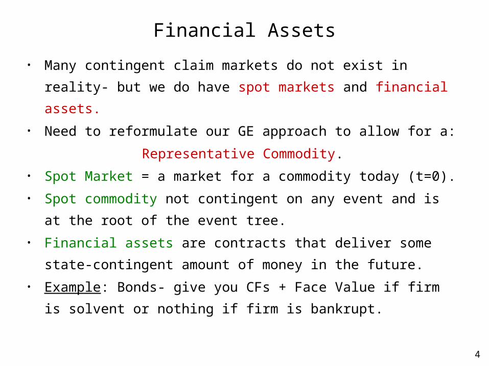
Financial Assets

• Many contingent claim markets do not exist in reality-

but we do have spot markets and financial assets.

• Need to reformulate our GE approach to allow for a:

Representative Commodity.

• Spot Market = a market for a commodity today (t=0).

• Spot commodity not contingent on any event and is at

the root of the event tree.

• Financial assets are contracts that deliver some state-

contingent amount of money in the future.

• Example: Bonds- give you CFs + Face Value if firm is

solvent or nothing if firm is bankrupt.

5

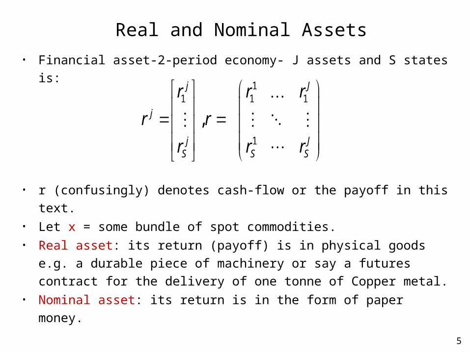
Real and Nominal Assets

• Financial asset-2-period economy- J assets and S states is:

• r (confusingly) denotes cash-flow or the payoff in this text.

• Let x = some bundle of spot commodities.• Real asset: its return (payoff) is in physical goods e.g. a

durable piece of machinery or say a futures contract for the delivery of one tonne of Copper metal.

• Nominal asset: its return is in the form of paper money.

11 1 1

1

,

j J

j

j JS S S

r r r

r r

r r r

6

Real and Nominal Assets (contd.)

• Let x = some bundle of spot commodities.

• Real asset: Cash flow is linear function of spot prices-

delivers the purchasing power necessary to buy some

specific commodity bundle x on tomorrow’s spot markets.

• Cash flows of some assets are independent of spot prices-

an example is a nominal bond.

• Bond delivers some specified (state-contingent) amount of

money.

• Nominal asset: delivers some specified amount of state-

contingent money- you cannot consume this money but

can spend it on buying some commodity but the

purchasing power is uncertain.

js sr p x

7

Arrow Securities

• Risk free asset is one that delivers a fixed amount of

money in all states. For a bond, lets fix this amount of

money to be = 1.• Arrow security - delivers one unit of purchasing power

conditional on an event s or zero otherwise.• Vector of state-contingent cash flows of a state s:

• Any financial asset can be represented by a portfolio

of Arrow securities.

1 0 0

0 1

0 0 1

0

1

0

,se e

8

Law of One Price

• Suppose there are no frictions – we also assume that the law of one price holds.

• LOP say that if two portfolios have the same payoffs they must cost the same or have the same price.

• Suppose the price of security j is qj and if two portfolios

have the same cash flows, they have the same price:

• We can write, the price of a security and a portfolio as:

• Risk free asset in Arrow world is:

r z r z q z q z

jjq r or q r

1 1 1

9

Aside on Real Vector Spaces• Consider a return matrix r and a vector of financial asset

prices q.

• Cost of a portfolio z= q.z, yields a cash flow =rs.z in state s

tomorrow.• Collecting all portfolios and tomorrow’s cash flows that

can be created in this way we get the market span:

(q) is a linear space of at most J dimensions- captures the choice set of agents. If two different return matrices and security price vectors give rise to the same market span they are equivalent- its only a change of basis.

-qspan

r

-q

r

q

z z

JR

M

10

Towards Radner Equilibrium

• In a contingent claim economy, demand equals supply for each

commodity in each state of equilibrium.

• What about an economy with financial assets? What does market

clearing mean for financial assets ?

• Every security bought by an investor must first be issued.

• If someone issues an asset he is short in this asset.

• Aggregating over all individuals the holdings must sum to zero-each

security bought by an individual must be sold by some one.

• Market clearing condition : Financial assets are in zero net supply.

• In partial equilibrium models you could have financial assets in

positive net supply.

• Example: Outstanding shares of a firm (in a model) can be taken as

given- if the firm is not an active player in the model, the short

position of the firm in its own shares is ignored and these shares are

in positive net supply for the rest of the economy.

11

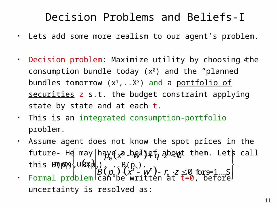
Decision Problems and Beliefs-I

• Lets add some more realism to our agent’s problem. • Decision problem: Maximize utility by choosing the

consumption bundle today (x0) and the “planned” bundles

tomorrow (x1,..XS) and a portfolio of securities z s.t. the

budget constraint applying state by state and at each t.• This is an integrated consumption-portfolio problem.• Assume agent does not know the spot prices in the future-

He may have a belief about them. Lets call this B(p1), B(p2),

..B(pS).

• Formal problem can be written at t=0, before uncertainty is

resolved as:

0 00

for s=1...,S

0max u x

0s ss s

p x w q z

B p x w r z

12

Decision Problems and Beliefs-II

• Combining the constraints in each period (and using the fact that

since the utility function monotonic the constraints bind with

equality- we can write the formal problem compactly at t=0, before

uncertainty is resolved as:

• Note that we ignore issues about the how people form

beliefs-we do above given some set of beliefs.• Later we will need to make an assumption about how beliefs

are formed.

max u x B p x q M

0 00

for s=1...,S

0max u x

0s ss s

p x w q z

B p x w r z

13

Plans, Prices and Price Expectations

• Prices = spot prices that can be observed today.• Plans = consumption bundles today and planned

consumption bundles in all states that will materialize

tomorrow.• Price Expectations = tomorrows prices where each agent

has some beliefs about these prices.• Here in addition to market clearing an equilibrium requires

that everyone has the same beliefs and that these beliefs

are correct or ps=Bi (ps) or “rational expectations”.

• A Radner equilibrium is a four-tuple:p=spot prices,

q=security prices, x(i) and z(i) collections of consumption

matrices and security portfolios for each I where: argmax u , 1ix i y B p y q i I M

14

Plans, Prices and Price Expectations• A Radner equilibrium is :

• Aggregate consumption equal aggregate endowment today and in each state tomorrow.

• Each security is in zero net supply:

• Everyone has perfect conditional foresight.

argmax u , 1ix i y B p y q i I M

1 1

, 0,1, , 1I I

s sm m

i i

x i i s S i I

1

0, 0,1,I

ji

z i j J

, 1... , 1.. ; 1..i m ms sB p p i I s S m M

15

Agent’s problem in Radner Economies-I

• In a Radner economy we can divide an agents decision problem into two: the consumption-composition problem and the financial problem.

• Here if we replace Bi{ps} with ps:

• Denoting with w the state-contingent value of the agent’s endowment, evaluated at spot prices:

• w0 is the agents income today and w1…ws , is his state-contingent future income.

max u x B p x q M

max u x p x q M

s=p 0,s sw s S

16

Agent’s problem in Radner Economies-II

• Define the indirect utility function v as:

• v(y) is the maximized utility if at most ys can be spent in state s. The choice of x is the choice about what commodities should be bought in each state.

• y=(y0,y1,…ys) is the distribution of incomes spent today and tomorrow in each state: summarizes the allocation of the financial means of the agent over time and across states. The choice of y is about savings and risk- the financial decision. The financial problem alone is :

v y =max u , 0,s ssx p x y for s S

max v y y w M q

17

Agent’s problem in Radner Economies-III

• Problem:• Requires the agent to maximize his indirect utility

function v over y subject to staying within the transfers that the market span allows or the same as

• The state-contingent budget constraints must be binding by the monotonicity of u and are thus satisfied by the equality.

max v y y w M q

max u x p x q M

max v y

max max u x

max u x

y w

p x y y w

p x

M q

M q

M q

18

Why are we doing all this work?

• Separation of the integrated consumption-portfolio problem

into a financial part and a consumption composition part can

be used to simplify the original economy (u,w,r).• Let (p,q,x,z) be an equilibrium of this economy.• Consider a new economy (v,w) where:

• This is a contingent claim economy with I agents but with

only one commodity- income or consumption – today and in

each of the future states.• Now again, as in the case of a representative agent, by using

a single representative good, we lose information; this time

on the composition of the consumption.

s=p 0,s sw s S

v y =max u , 0,s ssx p x y for s S

19

Complete Markets• Definition: We say that markets are complete if agents can

insure each state separately i.e. if they can trade assets in

such a way as to affect the payoff in one specific state without

affecting the payoff in other states.• When markets are complete the individual’s decision problem

in an asset economy is the same as in a contingent claim

economy.

Consequences of incompleteness• Arrow prices associated with equilibrium are not unique

(pricing of new assets that are not in the span of existing

assets is not well defined).• No unanimous production plan for firms (firms with dispersed

ownership lead to conflicts of objectives of owners).• The equilibrium allocation is not Pareto efficient- No locally

representative agent based on a SWF (aggregate models do

not exist).

20

Effects of Incomplete markets

• Complete markets financial markets are such that individual states can be insured.

• When markets are complete the individual’s decision problem in an asset economy is the same as in a contingent claim economy.

• Hence for every competitive equilibrium of an abstract exchange economy there is a corresponding economy with a Radner equilibrium.

• Equilibrium allocation same in contingent claim equilibrium and Radner equilibrium.

• Thus, welfare theorem holds also in an asset economy provide markets are complete.

• We can therefore construct the competitive SWF and the representative agent in the same way.

• But, can we construct the representative if market are incomplete?

21

Representative in an incomplete market?

• We cannot construct, in general, a representative if the market is incomplete? Why?

• Incomplete market return matrix is singular and the market space has less than S dimensions.

• Consequently some income transfers , from one state to another or one time period to another cannot be achieved independently of each other.

• This has profound effects for equilibrium- why?• FOC’s everyone’s marginal rates of state contingent

intertemporal substitution of wealth are given by Arrow prices.• But Arrow prices are not now defined uniquely in a Radner

equilibrium because there is an infinite combination of Arrow prices that are orthogonal to M(q).

• Different agents have different MRS’s and they would like to trade with each other because there are benefits from such trade.

22

Representative in an incomplete market?-II

• However they cannot perform this trade since the financial markets do not have the infrastructure to do so.

• Now there is no SWF that is maximized- hence the equilibrium allocation is not Pareto efficient.

• Lack of efficiency has grave implications for the equilibrium.

• Now no representative agent can be computed on the basis of a SWF.

• Does not affect – ideas like no arbitrage pricing but affects models like the SDF of the CCAPM etc. that we will develop.

• In an economy with production, people will not agree about production plans and shareholders will not agree about the best course of action for the firm or about delegation to management etc.

23

Effects of incomplete markets

• Arrow prices associated to an equilibrium are not unique.

• Typically, the equilibrium is not Pareto efficient.• Typically, there is no locally representative agent

based on a SWF.• Typically,there are no unanimous production plans

for firms.• Implying the following:• Prices of arbitrary new assets (not in the span of

the existing return matrix) are not well defined.• Aggregate models do not exist.• Multilateral ownership of a firm leads to conflict.

24

Quasi-complete markets

• An incomplete market economy could be accidentally

efficient!

• If the span of the incomplete market contains a Pareto-

efficient point-then this allocation is an equilibrium of

this economy which also happens to be efficient.

• Now all aggregations can be performed despite the

incompleteness-termed a quasi-complete market.

• Suppose x is a Pareto efficient allocation and a q s.t.

for each agent:

• Then we can say that the asset market r is quasi-complete

and then z such that (p,q,x,z) is Radner equilibrium.

• We can show now that goods and asset markets clear and

that everyone behaves optimally.

p x i i q M