1. Introduction Study of social systems using statistical ...sen/IJMPB-with-Alexandra-Battles.pdf · Study of social systems using statistical physics based approaches, or sociophysics,

April 24, 2017 15:15 IJMPB S0217979217420024 page 1

International Journal of Modern Physics BVol. 31, No. 10 (2017) 1742002 (14 pages)c� World Scientific Publishing CompanyDOI: 10.1142/S0217979217420024

Study of simple land battles using agent-based modeling:

Strategy and emergent phenomena

Alexandra Westley and Nicholas De Meglio

Department of Physics, SUNY Bu↵alo,Bu↵alo, New York, NY 14260–1500, USA

Rebecca Hager and Jorge Wu Mok

Department of Mathematics,SUNY Bu↵alo, Bu↵alo, New York, NY 14260-2900, USA

Linda Shanahan

Department of Physics, SUNY College at Bu↵alo,1300 Elmwood Avenue, Bu↵alo, New York, NY 14222, USA

Surajit Sen⇤

Department of Physics, SUNY at Bu↵alo,

Bu↵alo, New York, NY 14260–1500, USAsen@bu↵alo.edu

Received 16 October 2016Revised 28 November 2016Published 22 March 2017

In this paper, we expand upon our recent studies of an agent-based model of a battlebetween an intelligent army and an insurgent army to explore the role of modifyingstrategy according to the state of the battle (adaptive strategy) on battle outcomes. Thismodel leads to surprising complexity and rich possibilities in battle outcomes, especiallyin battles between two well-matched sides. We contend that the use of adaptive strategiesmay be e↵ective in winning battles.

Keywords: Cellular automata, battle, competition.

PACS numbers: 05.90.+m, 05.10.Gg, 89.75.Kd

1. Introduction

Study of social systems using statistical physics based approaches, or sociophysics,has been the subject of significant attention in recent years.1 The theoretical works

⇤Corresponding author.

1742002-1


A. Westley et al.

of Galam and collaborators on political events such as elections including the2016 election of Trump3,a have illustrated the predictive power of sociophysicalstudies. Studies of gang rivalries using statistical physics based approaches havealso emerged in recent years.2 Cellular automata4 or agent-based models5 and evenmolecular dynamics based studies6 have likewise proven to be a powerful tool tomodel the temporal evolution of various complex systems.7,8 While technically sim-ple to set up, these models often can reveal deep insights into the dynamics of com-plex systems such as those alluded to below, behaviors that may not be discernibleusing traditional di↵erential equation based models.7

Cellular automata have naturally found applications in modeling such diversephenomena as crowd behavior,9,10 emergent behavior of an organization under spe-cific conditions,11 market behavior,12 in capturing the success of competing brandsor products in the market,13 in successfully describing the spread and mitigationof epidemics such as bird flu in poultry,14,15 and in describing the struggle betweenanimal species for territory and resources.16 Here, we use an agent-based approachto examine simple land battles, and explore various e↵ects of initial conditions andstrategy on the evolution and the outcome of such battles.17,18 Our battle modelcurrently describes a conflict between two species, though it is possible to extendthis to multiple species (see e.g., Ref. 19).

We construct a simple physical model consisting of a two-dimensional squarelattice or matrix and simple deployment rules.17,18 The symbols we use in thisstudy are introduced in Table 1 so that the work is easier to follow. The latticerepresents the battlefield on which conflict takes place. Individual attackers anddefenders are assigned numeric strength values and initially placed in the reserves.The simulations involve deployment strategies which result in occupation of thearray sites by the combatants. Casualties result when opposing forces occupy thesame site. Combatants do not actually move on the battlefield, but rather occupytheir given sites, engage intruders, and provide field information which may be usedfor determining the positioning of troops or agents in future iterations. Battlescontinue until either the attackers or the defenders have exhausted their reserveforces, or alternatively until either the attackers or defenders have gained controlof the entire battlefield. If both sides have essentially deployed all forces to theconflict, the battle is a draw. While this win/loss definition is somewhat arbitrary,it allows for a general discussion of results. To measure a victory numerically, weuse a so-called win/loss ratio � as defined in Eq. (3).

2. Model Details

Let us begin by considering a simple battle on a square lattice of sides L = 5.At the start of the battle, each side is allotted an initial reserve of A

0

= D0

=

aIt is interesting to see how Galam correctly projected the strong possibility of Trump becomingthe President-elect of the US nearly ten months in advance when the US polls largely failed tomake the correct projection. See S. Galam, in this issue.

1742002-2


Study of simple land battles using agent-based modeling

Table 1. Description of notation used.

L is the length of each side of the square latticeA0, A initial/final attack reservesD0, D initial/final defense reserves⇢A, ⇢D attack/defense densitya, d attack (negative), defense (positive) force levelR sight range (number of cells)r sight range (percentage of battlefield size)� win–loss ratio

5000 which may represent weapons, resources, troops, or any other logistical factor(see Table 1). A and D, respectively, denote the numbers of “attackers” and the“defenders” at any given time other than at the initiation point; we distinguishthem by means of the strategy each uses. To initialize the battle, we randomlyplace the defender’s force on the battlefield. This is done by taking a fixed numberof agents from their initial reserve D

0

and placing them randomly upon the lattice(with a given density ⇢D which is the ratio of sites occupied by the defenders tothe total number of sites on the lattice). Assuming that the defenders have variousforms of weapons and ammunitions, the deployment is done such that there is amix of strength values of, say, d = +1 and d = +2.b After this step, each latticesite K(i, j) = 0, 1, or 2.

The battle then begins with the attackers deploying in random locations on thebattlefield with their own occupation density ⇢A, with strength values of a = �1and a = �2. We pause to note that this is what we will refer to as a “symmetric”battle, since the strength value distributions of the attackers and defenders areequal in magnitude.

Following this initial deployment, some fraction of the sites will now have nega-tive values, indicating they are now held by the attackers. On subsequent iterations,the attackers and defenders will continue to draw from their respective reserves ac-cording to di↵erent algorithms. One can envision that such reserves are pulled fromdistributed command/control centers where reserve forces await.

Figure 1 shows an example randomized lattice at the start of a battle on a5⇥5 lattice. For our first example, we will use a random strategy for defenders andan intelligent, aggressive strategy for the attackers. This is inspired by the recentconflicts in Iraq; we choose to study the case of an insurgent army with access acrossthe entire battlefield and formidable knowledge of the terrain (and therefore highlycapable of making unpredictable or random attacks), versus an “intelligent” armywhose decision-making is limited by information regarding the distributions of theattackers and the defenders.

bIt is interesting to observe that the values of d and a are roughly connected to nature of armsavailable in the battle. Thus, d = +1 or a = �1, etc. would mean relatively simple weapons whereasd = +2, etc. would correspond to the availability of weapons that can cause more casualties.

1742002-3


A. Westley et al.

(a) (b)

Fig. 1. (a) The initial randomized state of a battle on a square lattice of sides L = 5. (b) Thefinal state, after reserves have been depleted for the defenders.

The defenders will continue to deploy their reserves as in the first step through-out the battle, by randomly selecting lattice sites with probability ⇢D and placingrandomly d = +1 or d = +2 on that site on each iteration.

For the attackers, it is important to know where the greatest density of defend-ers are located on the lattice. This knowledge requires intelligence regarding thecurrent state of the battlefield and this intelligence turns out to be important indetermining whether the attackers can overpower their opponents. In our studiesdiscussed below, the attackers take an aggressive approach by always deploying re-sources in the direction with the greatest density of defenders though, as we shallsee later, the reverse (defensive) strategy of retreating from the regions of greatestdensity of defenders can also turn out to be an e↵ective strategy in some cases. Wedefine a neighbor list by an n⇥m matrix about each attack site, KA(i, j). The sizeof the neighbor list is dictated by the range variable R, the number of lattice cells inany direction for which information is available at site KA. For an L⇥L matrix, wemay also measure the range as a fraction of lattice size: |r| = R

L (100)%. The attack-ers receive information from a neighbor list with maximum size (2R+1)⇥ (2R+1).The occupation or resource values of all sites in each quadrant of the neighbor listat KA(i, j) are summed. If the computed sum is largest in, say, the first quadrant,then site in which the attackers will be deployed to is

K(i+ 1, j + 1) ! K(i+ 1, j + 1) + amax

, (1)

(if this site is still within the battlefield) and so on. If adjacent quadrants, forexample quadrants I and II, have equal values

K(i, j + 1) ! K(i, j + 1) + amax

. (2)

1742002-4



Observe here that a larger value of R implies averaged and hence less precise

information over a larger area of a quadrant. Further, if R is very small, thattoo would imply limited intelligence about the immediate battlefield environment.Hence very small Rs are typically not very meaningful for our purposes. Simplyput, larger R implies limited battlefield intelligence whereas small R would typicallyimply strong local battlefield intelligence.

If opposing quadrants (i.e., I and III, or II and IV) or if three or even all fourquadrants of the neighbor list have the same value, there is no new deploymentfrom that site during that particular iteration (however, this case seldom occurs).The rationale for using maximum strength values for the attackers is their strategicneed to maximize e↵ectiveness. The battlefield is not updated until all such decisionshave been made.

At each iteration, these deployments repeat until at least one of the initialreserves A

0

or D0

has been completely depleted; at this point the battle ends, andwe must decide who has won!

For convenience, we will measure the magnitude of a victory by means of thesingle number �, the win–loss ratio, defined as follows:

� =

8>>>><

>>>>:

�1, ⇢D = 0 ,

+1, ⇢A = 0 ,

D �A

D0

+A0

otherwise .

(3)

This definition serves to measure victory of two types: by total territory control,or by depletion of reserves. Furthermore, the more lopsided the victory toward oneside, the larger a value � will take. Figure 1 shows the initial and final latticedistributions of a simple battle of the type described above.

For the rest of this paper, all battles will take place upon a 50⇥50 lattice unlessotherwise noted; on a lattice as small as the one above, the intelligent strategyof the attackers is nearly irrelevant due to the neighbor list covering most of thelattice! We have also studied lattice sizes that are large as L = 2500 and found thatdealing with such large systems increases the computation times needed but has nomeasurable e↵ect on the battle outcomes.

3. Strategy

We use the term “strategy” very broadly; it represents the force composition andthe behavior of one side, as well as their set of reactions to enemy moves. Ouroverall objective with strategy adjustment is to find a way to optimize one side’schances of winning; that is, the best ways to use intelligence to win a symmetricbattle.

1742002-5


A. Westley et al.

3.1. Initial conditions

Let us begin by studying the simple battle described in the previous section withaggressive (as opposed to defensive), intelligent attackers, but placed in a largerlattice. Here we wish to study the initial conditions that lead to a high probabilityfor the attackers to win. We note that the simulation is susceptible to di↵erentvictory/loss outcomes from di↵erent seeds of the random number generator; forthis reason, whenever a battle with certain initial conditions is mentioned, we aredescribing an average result taken over seven battles with di↵erent seeds.

To do this numerically, we examine the decay of the attackers’ reserves (denotedby A

0

for initial and by A for instantaneous values including the final value when thesimulation ends) as a function of the parameters (i) sight range, (ii) initial attackdensity, and (iii) initial defense density. The battles we studied were with symmetricforce levels a, d = �1, +1; �2, +2; and �3, +3; and asymmetric battles with forcelevels a, d = �2, +5; �3, +5; and �4, +5 (e.g., for �2, +5, a = �2, �1 and d = +1,+2, +3, +4, +5 are possible deployment values). The symmetric battles representtwo armies with matched weapons, equipment, and reserves; the asymmetric battlesgive one side an advantage in terms of e↵ectiveness of the attacks.

After some trial and error, we ended up varying the following parameters (seeTable 1) through the following ranges:

0.2 ⇢A 0.85 ,

0.2 ⇢D 0.85 ,

1 R 20 ,

where ⇢D is held fixed at all times whereas ⇢A is fixed at t = 0 and allowed to evolve

based on the evolution of the battle. Henceforth, unless otherwise specified, by ⇢Awe mean ⇢A(t = 0).

These limits on the densities ⇢A and ⇢D of attackers or defenders on the latticeexclude uninteresting combinations of ⇢A, ⇢D and R. For instance, places where theattackers deploy so few troops that they lose the battle within one or two iterations.Since R is the sight range in number of cells, it must be an integer (for perspective,20 cells is 40% of the L = 50 lattice battlefield.)

Let us assume that the attackers take a small fraction of agents from the initialreserves for every deployment and keep repeating this process until the reservesare depleted. Let us further assume that A would depend on the range R withA depleting more rapidly as R grows. Pretending for now that R is a continuousvariable (and R ! 0 is feasible) it would be reasonable to assume dA/dR = �↵A,where ↵ is some constant that depends on ⇢A and ⇢D. Then one can write

Z A

A0

dA0

A0 = �↵

Z R

0

dR0

or A = A0

exp(�↵R) ,

(4)

1742002-6



Fig. 2. log(A) versus R, with several di↵erent values for the initial value of ⇢A.

where the primes in Eq. (4) denote dummy variables. The parameter ↵, then, tellsus how strongly the outcome of the battle is coupled to the sight range parameterfor the chosen attack density. Equation (4) suggests that when the sight range istoo high, the attackers su↵er very high losses. Figure 2 presents the results fromour simulations which show that the exponential decay above provides a reasonabledescription of how A decays as a function of R. Observe that ↵ would have a highermagnitude if ⇢A is smaller.

Let us look closely at the decay parameter ↵(⇢A, ⇢D) which controls how thereserves of the attackers get depleted. As ⇢D becomes large and ⇢A becomes small,A ⇡ A

0

, which means that attackers cannot deploy any troops. This occurs becausethe field is so concentrated with defenders that the attackers cannot find a place todeploy. In the opposite limit, ⇢D is small and ⇢A is large; A ⇡ 0. This is caused by alack of defenders in the field, which will make attacker’s territory occupancy quicklygrow — leading them to either win by capturing all territory, or lose by runningout of reserves too quickly. So, for fixed initial conditions, we can summarize whatthe outcome of the battle will be in terms of the single parameter ↵.

Our simulations show that ↵ itself undergoes an exponential decay as a functionof ⇢D

⇢kA

as (see Fig. 3)

ln |↵| = ��⇢D⇢Ak

+ � , (5)

|↵| = exp(�) exp

✓� �

⇢D⇢kA

◆. (6)

� and � are positive constants for a given symmetric force level, and k is approxi-mately 0.20, for all cases analyzed.

1742002-7


A. Westley et al.

Fig. 3. ↵, the decay parameter of Fig. 2, as a function of defense density ⇢D.

Combining Eqs. (4) and (6),

A = A0

exp

✓�Cr exp

✓��

⇢D⇢Ak

◆◆, (7)

where C ⌘ exp(�). Equation (7) summarizes how the attackers’ reserves will behaveas r, ⇢D, and ⇢A change.

We find therefore that the outcome of the battle for the aggressive attackersdepends greatly on moderation: one must have some local knowledge, but not toomuch! One must deploy enough troops from reserves, but not too many! We nextbriefly summarize our studies on the e↵ectiveness of the defensive strategy [seediscussion above Eq. (1)] before moving on to the strengths and weaknesses ofvarious mixed strategies.

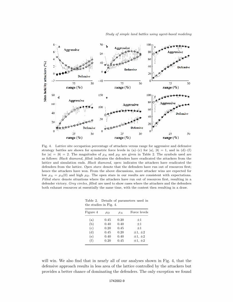
Figure 4 summarizes the results from a large number of studies determininghow much territory has been acquired by the attackers for varying r given di↵erent⇢A, ⇢D and strategies, i.e., whether aggressive or defensive. In Figs. 4(a)–4(c),|a| = |b| = 1, and in Figs. 4(d)–4(f), |a| = |b| = 2. Each point represents theaverage of three runs with associated error bars. In each panel, the percentage ofsites held by the attackers is shown versus r for fixed values of ⇢A(0) and ⇢D. Inpanels (a) and (d) we have used ⇢A = 0.2, ⇢D = 0.45, in (b) and (e) ⇢A = 0.40,⇢D = 0.40, and in (c) and (f) ⇢A = 0.45, ⇢D = 0.20. We summarize the results asfollows:

When |a| = |b| = 2, the conflict outcomes become more sensitive to the value of rand to whether an aggressive or defensive strategy is used. Our studies suggest thatwhen the defenders are highly exposed to attacks, but not so high as to exhaust thereserves too quickly, such as in Figs. 4(c) and 4(f), it is less likely that the attackers

1742002-8



Fig. 4. Lattice site occupation percentage of attackers versus range for aggressive and defensivestrategy battles are shown for symmetric force levels in (a)–(c) for |a|, |b| = 1, and in (d)–(f)for |a| = |b| = 2. The magnitudes of ⇢A and ⇢D are given in Table 2. The symbols used areas follows: Black diamond, filled: indicates the defenders have eradicated the attackers from thelattice and simulation ends. Black diamond, open: indicates the attackers have eradicated thedefenders from the lattice. Open stars: denote that the defenders have run out of resources first;hence the attackers have won. From the above discussions, more attacker wins are expected forlow ⇢A = ⇢A(0) and high ⇢D. The open stars in our results are consistent with expectations.Filled stars: denote situations where the attackers have run out of resources first, resulting in adefender victory. Grey circles, filled: are used to show cases where the attackers and the defendersboth exhaust resources at essentially the same time, with the contest then resulting in a draw.

Table 2. Details of parameters used inthe studies in Fig. 4.

Figure 4 ⇢D ⇢A Force levels

(a) 0.45 0.20 ±1(b) 0.40 0.40 ±1(c) 0.20 0.45 ±1(d) 0.45 0.20 ±1, ±2(e) 0.40 0.40 ±1, ±2(f) 0.20 0.45 ±1, ±2

will win. We also find that in nearly all of our analyses shown in Fig. 4, that thedefensive approach results in less area of the lattice controlled by the attackers butprovides a better chance of dominating the defenders. The only exception we found

1742002-9


A. Westley et al.

is when the attackers have low exposure and high local intelligence and the forcelevels are minimal, a defensive strategy works better in winning and in establishingterritorial dominance in favor of attackers. We note from the error bars that thee↵ects of randomness on the spatial and force outcomes increase with increasing⇢A and with increasing attack strength.

From here, we will seek to further optimize these battles by adjusting the at-tackers’ strategy — for example, is it possible to reduce that minimum deploymentdensity ⇢A in order to reduce losses? This and more will be discussed in the followingsection.

3.2. Mid-battle strategies

In a basic battle, the attackers’ strategy is very simple. Both sides initially deployrandomly; the defenders continue to do so for the duration, but the attackers deployreinforcements in the direction of high defender concentrations. This is what we hadcalled an aggressive strategy. A defensive strategy is the opposite; attackers deployin the opposite direction of enemy concentrations (i.e., they always retreat).

The aggressive strategy tends to be excellent for capturing territory, but takesheavy losses to do so. The defensive strategy has the opposite e↵ect; it cannotcapture territory well, but it minimizes losses. Our initial attempt using a mix ofstrategies was simply to vary the aggressiveness of the attackers during the courseof the simulation. For example, have the attackers flip a coin at each iteration todecide whether they will use an aggressive or defensive strategy. However, aftersome testing, we found that this is an ine↵ective strategy; it shows the weaknessesof both of the aggressive and defensive strategies, but does not adequately capturetheir strengths. The studies hence suggested that actions must be based on soundlogic aimed at neutralizing the enemy rather than taking chances with what couldbe ine↵ective moves.

To improve the adaptive strategy approach, we made it more active. We de-signed the strategy to hold site occupation between 20 and 80% of the battlefield;from previous work, this is a favorable region of the phase space for the attackers(see Figs. 9–11 in Ref. 20). The mechanics are simple: when site occupation is low,we increase the attackers’ force level and aggressiveness, as if they had broughtheavier weapons from a reserve. When site occupation is too high (i.e., they be-come overextended), we switch the attackers’ strategy to fully defensive. We haveobserved that this causes them to retreat into small (2⇥ 2 or 3⇥ 3) regions of hightroop density — fortified positions, in e↵ect.

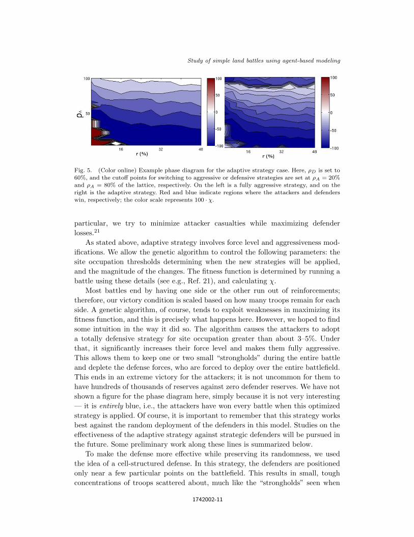
Unlike the much simpler mixed strategy, the adaptive strategy is very powerful;it results in attacker victories in many regions of the phase diagram where theywould normally have lost. See Fig. 5 for an example.

This strategy still is not quite optimized, however; at a defense density near40%, the attackers still nearly always lose despite their cleverness. We use a geneticalgorithm to quickly search through the space to find a winning strategy — in

1742002-10



Fig. 5. (Color online) Example phase diagram for the adaptive strategy case. Here, ⇢D is set to60%, and the cuto↵ points for switching to aggressive or defensive strategies are set at ⇢A = 20%and ⇢A = 80% of the lattice, respectively. On the left is a fully aggressive strategy, and on theright is the adaptive strategy. Red and blue indicate regions where the attackers and defenderswin, respectively; the color scale represents 100 · �.

particular, we try to minimize attacker casualties while maximizing defenderlosses.21

As stated above, adaptive strategy involves force level and aggressiveness mod-ifications. We allow the genetic algorithm to control the following parameters: thesite occupation thresholds determining when the new strategies will be applied,and the magnitude of the changes. The fitness function is determined by running abattle using these details (see e.g., Ref. 21), and calculating �.

Most battles end by having one side or the other run out of reinforcements;therefore, our victory condition is scaled based on how many troops remain for eachside. A genetic algorithm, of course, tends to exploit weaknesses in maximizing itsfitness function, and this is precisely what happens here. However, we hoped to findsome intuition in the way it did so. The algorithm causes the attackers to adopta totally defensive strategy for site occupation greater than about 3–5%. Underthat, it significantly increases their force level and makes them fully aggressive.This allows them to keep one or two small “strongholds” during the entire battleand deplete the defense forces, who are forced to deploy over the entire battlefield.This ends in an extreme victory for the attackers; it is not uncommon for them tohave hundreds of thousands of reserves against zero defender reserves. We have notshown a figure for the phase diagram here, simply because it is not very interesting— it is entirely blue, i.e., the attackers have won every battle when this optimizedstrategy is applied. Of course, it is important to remember that this strategy worksbest against the random deployment of the defenders in this model. Studies on thee↵ectiveness of the adaptive strategy against strategic defenders will be pursued inthe future. Some preliminary work along these lines is summarized below.

To make the defense more e↵ective while preserving its randomness, we usedthe idea of a cell-structured defense. In this strategy, the defenders are positionedonly near a few particular points on the battlefield. This results in small, toughconcentrations of troops scattered about, much like the “strongholds” seen when

1742002-11


A. Westley et al.

the attackers use an adaptive strategy. The di↵erence here is that a cell may bedefeated if its leader is killed; that is, if the attackers manage to penetrate to thecenter of the cell, defenders stop deploying there. Against any enemy short of thegenetic algorithm based optimization strategy, this leads to a victory for the defense.

To adjust for the cell defense, we used a strategy called “smart deployment” forthe attackers. This strategy assumes that the attackers have excellent intelligenceof the battlefield, and causes them to deploy only in regions where there is a heavyenemy presence. It completely countered the cell structure, returning our battlesto a contested state. The reason for this result is twofold: first, it was applied toan army that has local intelligence. This allows the attackers to quickly locate anddeploy near the main concentrations. Second, the battlefield is far emptier than ina basic battle; since the defenders only control the immediate area around theircells, the attackers can gain the benefit of not deploying in the empty areas.

The battle with cell-structured defense and smart-deploying attackers has manyinteresting behaviors. The attackers surround defense concentrations, cut throughlines, and push forward to the center of the cells. Figure 6 shows a snapshot takenfrom one of these battles.

Fig. 6. (Color online) An intelligent attacker using smart deployment against a cell-based defense.Black represents defenders, gray represents attackers, and white cells are neutral.

1742002-12



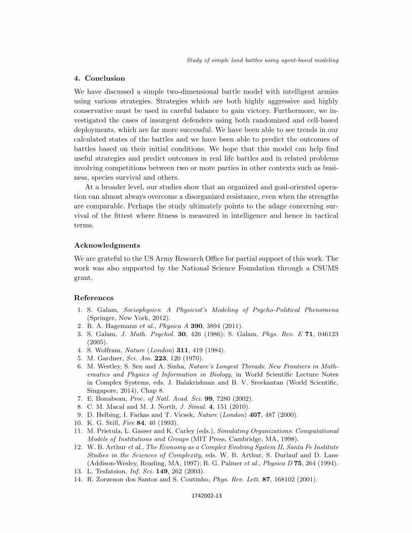
4. Conclusion

We have discussed a simple two-dimensional battle model with intelligent armiesusing various strategies. Strategies which are both highly aggressive and highlyconservative must be used in careful balance to gain victory. Furthermore, we in-vestigated the cases of insurgent defenders using both randomized and cell-baseddeployments, which are far more successful. We have been able to see trends in ourcalculated states of the battles and we have been able to predict the outcomes ofbattles based on their initial conditions. We hope that this model can help finduseful strategies and predict outcomes in real life battles and in related problemsinvolving competitions between two or more parties in other contexts such as busi-ness, species survival and others.

At a broader level, our studies show that an organized and goal-oriented opera-tion can almost always overcome a disorganized resistance, even when the strengthsare comparable. Perhaps the study ultimately points to the adage concerning sur-vival of the fittest where fitness is measured in intelligence and hence in tacticalterms.

Acknowledgments

We are grateful to the US Army Research O�ce for partial support of this work. Thework was also supported by the National Science Foundation through a CSUMSgrant.

References

1. S. Galam, Sociophysics: A Physicist’s Modeling of Psycho-Political Phenomena(Springer, New York, 2012).

2. R. A. Hagemann et al., Physica A 390, 3894 (2011).3. S. Galam, J. Math. Psychol. 30, 426 (1986); S. Galam, Phys. Rev. E 71, 046123

(2005).4. S. Wolfram, Nature (London) 311, 419 (1984).5. M. Gardner, Sci. Am. 223, 120 (1970).6. M. Westley, S. Sen and A. Sinha, Nature’s Longest Threads: New Frontiers in Math-

ematics and Physics of Information in Biology, in World Scientific Lecture Notesin Complex Systems, eds. J. Balakrishnan and B. V. Sreekantan (World Scientific,Singapore, 2014), Chap 8.

7. E. Bonabeau, Proc. of Natl. Acad. Sci. 99, 7280 (2002).8. C. M. Macal and M. J. North, J. Simul. 4, 151 (2010).9. D. Helbing, I. Farkas and T. Vicsek, Nature (London) 407, 487 (2000).

10. K. G. Still, Fire 84, 40 (1993).11. M. Prietula, L. Gasser and K. Carley (eds.), Simulating Organizations: Computational

Models of Institutions and Groups (MIT Press, Cambridge, MA, 1998).12. W. B. Arthur et al., The Economy as a Complex Evolving System II, Santa Fe Institute

Studies in the Sciences of Complexity, eds. W. B. Arthur, S. Durlauf and D. Lane(Addison-Wesley, Reading, MA, 1997); R. G. Palmer et al., Physica D 75, 264 (1994).

13. L. Tesfatsion, Inf. Sci. 149, 262 (2003).14. R. Zorzenon dos Santos and S. Coutinho, Phys. Rev. Lett. 87, 168102 (2001).

1742002-13


A. Westley et al.

15. T. Kim et al., Europhys. Lett. 86, 24002 (2009).16. R. Smith and M. Bedau, Evol. Comput. 8, 419 (2000).17. L. Shanahan and S. Sen, Int. J. Mod. Phys. E 17, 930 (2008).18. L. Shanahan and S. Sen, Mod. Phys. Lett. B 25, 2279 (2011).19. J. Epstein, Proc. Natl. Acad. Sci. USA 99, 7243 (2002).20. L. Shanahan, PhD Thesis, SUNY Bu↵alo (2011).21. T. Baker et al., Proc. of SPIE 5649, 574 (2005).

1742002-14

Documents

1. Introduction Study of social systems using statistical ...sen/IJMPB-with-Alexandra-Battles.pdf · Study of social systems using statistical physics based approaches, or sociophysics,