Embed Size (px)
Citation preview
Wei-Ta Chu
Introduction of Audio Signals1
2010/11/25
Multimedia Content Analysis, CSIE, CCU
Li and Drew, Fundamentals of Multimedia, Prentice Hall, 2004

Announcement2
� Project proposal: Dec. 9, 2010
� Each team can be formed by 1~3 persons
� Each team presents idea for about 15 minutes
� Discuss with me before you propose.
Multimedia Content Analysis, CSIE, CCU
� You can find me each afternoon. (Nov. 26~Dec.3, except for Dec. 1)

Sound3
� Sound is a wave phenomenon like light, but is macroscopic and involves molecules of air being compressed and expanded under the action of some physical device.
� Since sound is a pressure wave, it takes on continuous values, as opposed to digitized ones.
Multimedia Content Analysis, CSIE, CCU
as opposed to digitized ones.

Digitization4
� Digitization means conversion to a stream of numbers, and preferably these numbers should be integers for efficiency.
� Sampling and Quantization
Multimedia Content Analysis, CSIE, CCU
Sampling and Quantization

Digitization5
� The first kind of sampling, using measurements only at evenly spaced time intervals, is simply called, sampling. The rate at which it is performed is called the sampling frequency.
� For audio, typical sampling rates are from 8 kHz (8,000 samples per second) to 48 kHz. This range is determined by
Multimedia Content Analysis, CSIE, CCU
samples per second) to 48 kHz. This range is determined by Nyquist theorem discussed later.
� Typical uniform quantization rates are 8-bit and 16-bit. 8-bit quantization divides the vertical axis into 256 levels, and 16-bit divides it into 65536 levels.
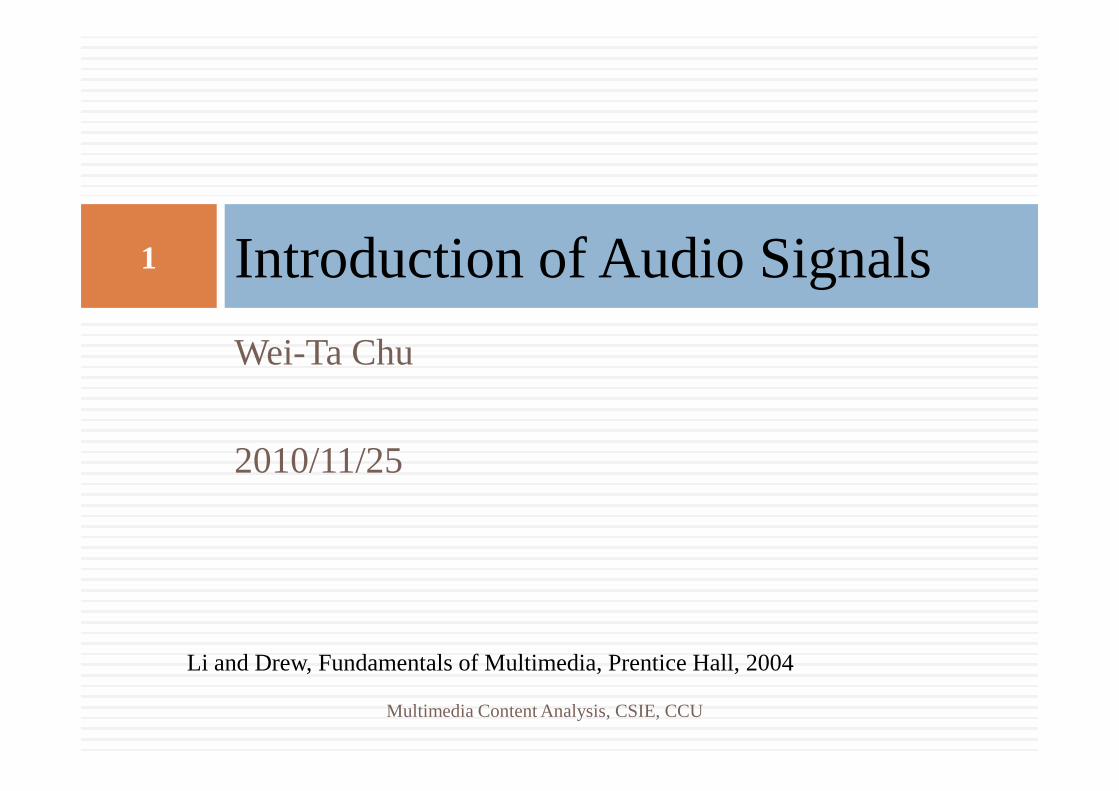
Sinusoids6
Multimedia Content Analysis, CSIE, CCU
Nyquist Theorem7
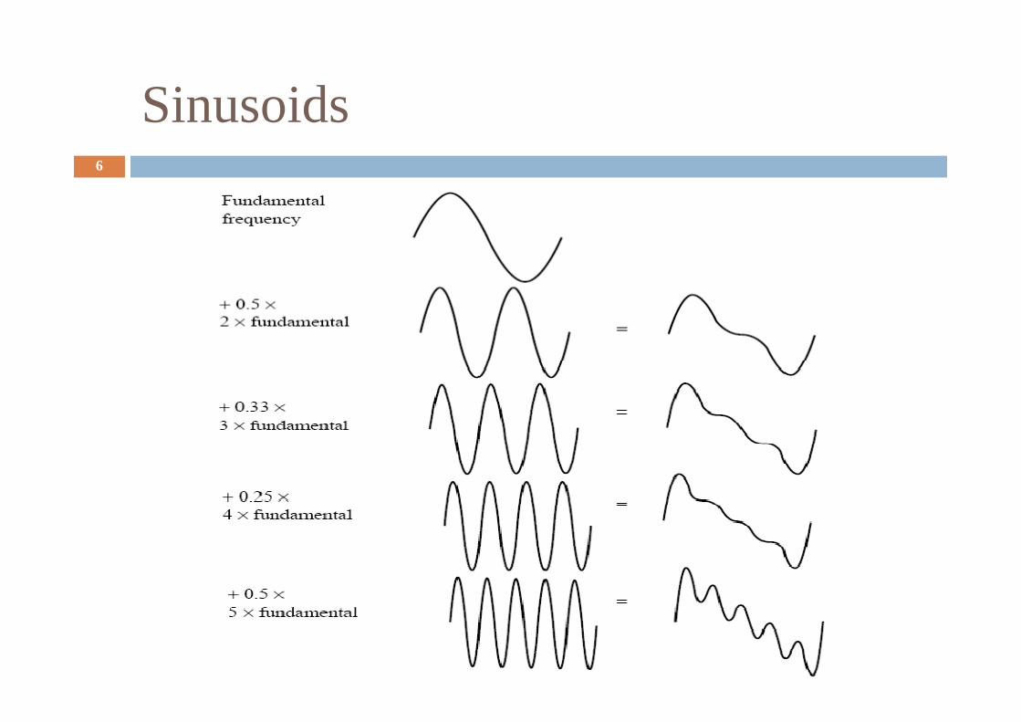
� The Nyquist theorem states how frequently we must sample in time to be able to recover the original sound.
� If sampling rate just equals the actual frequency, this figure shows that a false signal is detected: it is simply a constant, with zero frequency. with zero frequency.

Nyquist Theorem8
� If sample at 1.5 times the actual frequency, this figure shows that we obtain an incorrect (alias) frequency that is lower than the correct one.
� For correct sampling we must use a sampling rate equal to at least twice the maximum frequency content in the signal. This least twice the maximum frequency content in the signal. This rate is called the Nyquist rate.
Nyquist Theorem9
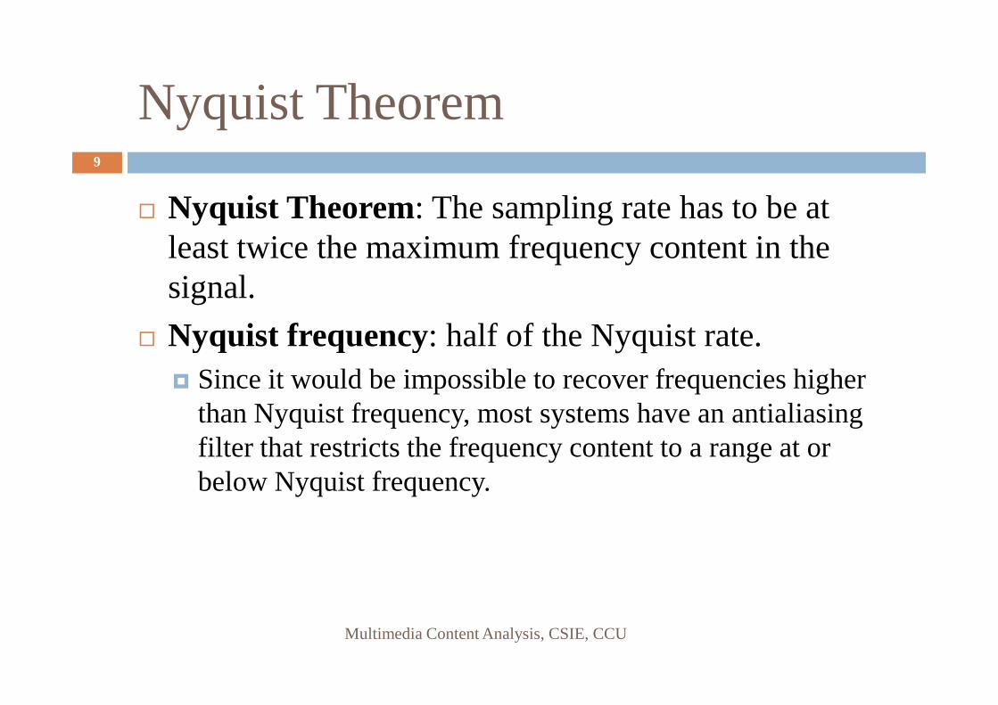
� Nyquist Theorem: The sampling rate has to be at least twice the maximum frequency content in the signal.
� Nyquist frequency: half of the Nyquistrate.
Multimedia Content Analysis, CSIE, CCU
Nyquist frequency: half of the Nyquistrate.� Since it would be impossible to recover frequencies higher
than Nyquist frequency, most systems have an antialiasingfilter that restricts the frequency content to a range at or below Nyquist frequency.

Signal-to-Noise Ratio (SNR)10
� The ratio of the power of the correct signal and the noise is called the signal to noise ratio (SNR) - a measure of the quality of the signal.
� The SNR is usually measured in decibels (dB), where 1 dB is a tenth of a bel. The SNR value, in units of dB, is defined in
Multimedia Content Analysis, CSIE, CCU
a tenth of a bel. The SNR value, in units of dB, is defined in terms of base-10 logarithms of squared voltages, as follows:
� If the signal voltage Vsignal is 10 times the noise, the SNR is
Signal-to-Quantization-Noise Ratio (SQNR)
11
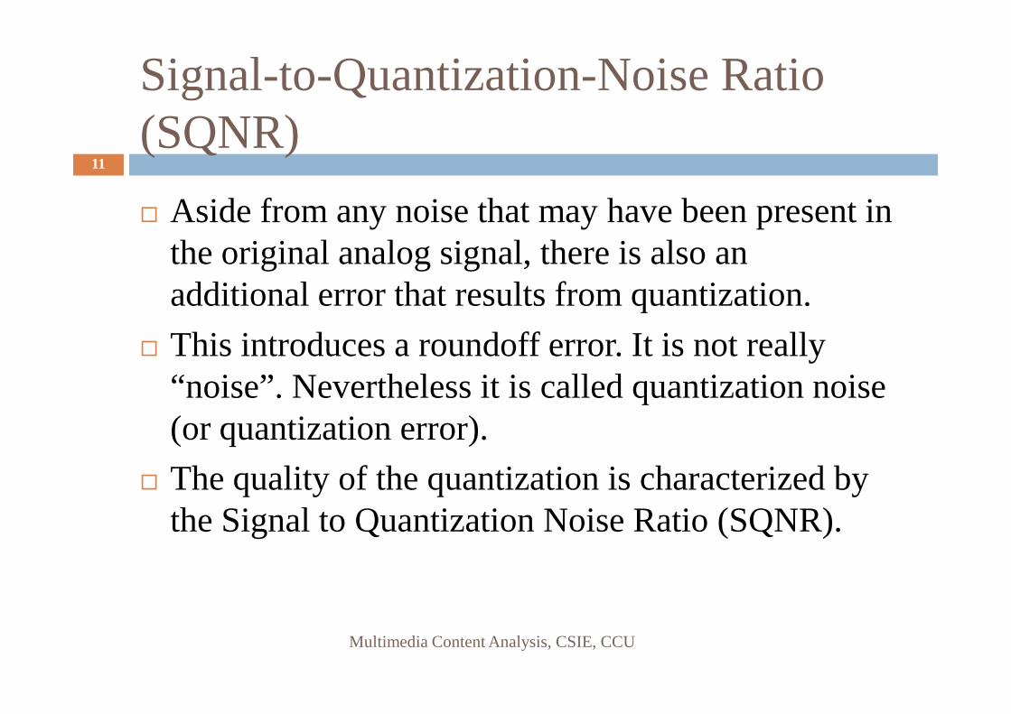
� Aside from any noise that may have been present in the original analog signal, there is also an additional error that results from quantization.
� This introduces a roundofferror. It is not really
Multimedia Content Analysis, CSIE, CCU
� This introduces a roundofferror. It is not really “noise”. Nevertheless it is called quantization noise (or quantization error).
� The quality of the quantization is characterized by the Signal to Quantization Noise Ratio (SQNR).

Signal-to-Quantization-Noise Ratio (SQNR)
12
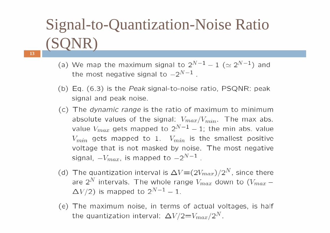
� For a quantization accuracy of N bits per sample, the range of the digital signal is -2N-1 to 2N-1-1.
� If the actual analog signal is in the range from –Vmaxto +Vmax, each quantization level represents a voltage of 2Vmax/2N, or Vmax/2N-1
Multimedia Content Analysis, CSIE, CCU
of 2Vmax/2N, or Vmax/2N-1
� Peak SQNR
Signal-to-Quantization-Noise Ratio (SQNR)
13
Multimedia Content Analysis, CSIE, CCU

Signal-to-Quantization-Noise Ratio (SQNR)
14
� 6.02N is the worst case. If the input signal is sinusoidal, the quantization error is statistically independent, and its magnitude is uniformly distributed between 0 and half of the interval, then it can be shown that the expression for the SQNR becomes
Multimedia Content Analysis, CSIE, CCU
SQNR becomes
� Typical digital audio sample precision is either 8 bits per sample, equivalent to about telephone quality, or 16 bits, for CD quality.
Linear and Nonlinear Quantization15
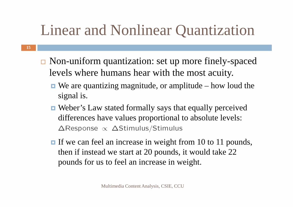
� Non-uniform quantization: set up more finely-spaced levels where humans hear with the most acuity. � We are quantizing magnitude, or amplitude – how loud the
signal is.
Weber’s Law stated formally says that equally perceived
Multimedia Content Analysis, CSIE, CCU
� Weber’s Law stated formally says that equally perceived differences have values proportional to absolute levels:
� If we can feel an increase in weight from 10 to 11 pounds, then if instead we start at 20 pounds, it would take 22 pounds for us to feel an increase in weight.

Linear and Nonlinear Quantization16
Multimedia Content Analysis, CSIE, CCU
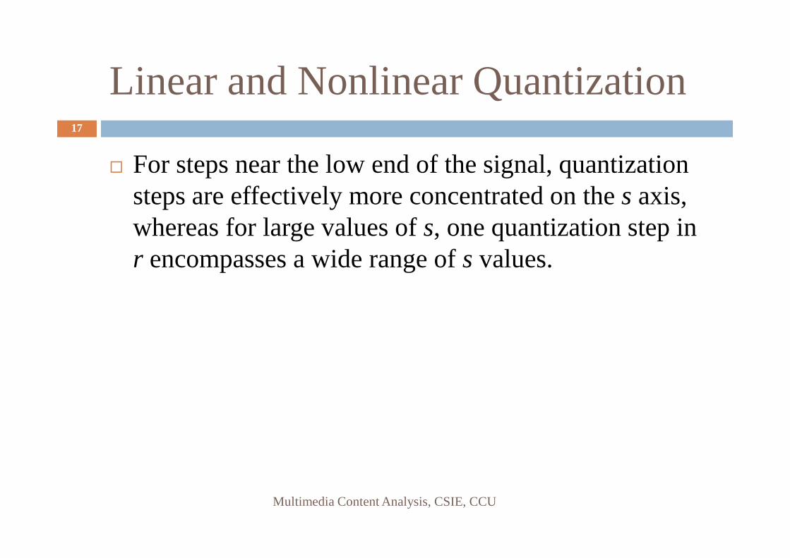
Linear and Nonlinear Quantization17
� For steps near the low end of the signal, quantization steps are effectively more concentrated on the s axis, whereas for large values of s, one quantization step in r encompasses a wide range of s values.
Multimedia Content Analysis, CSIE, CCU

Linear and Nonlinear Quantization18
Multimedia Content Analysis, CSIE, CCU
sp is the peak signal value and s is the current signal value

Linear and Nonlinear Quantization19
Multimedia Content Analysis, CSIE, CCU

Audio Filtering20
� Prior to sampling and analog-to-digital conversion, the audio signal is also usually filtered to remove unwanted frequencies.
� For speech, typically from 50Hz to 10kHz is retained, and other frequencies are blocked by the use of a band-pass filter that screens out lower and higher frequencies.
Multimedia Content Analysis, CSIE, CCU
that screens out lower and higher frequencies.
� An audio music signal will typically contain from about 20Hz up to 20kHz.
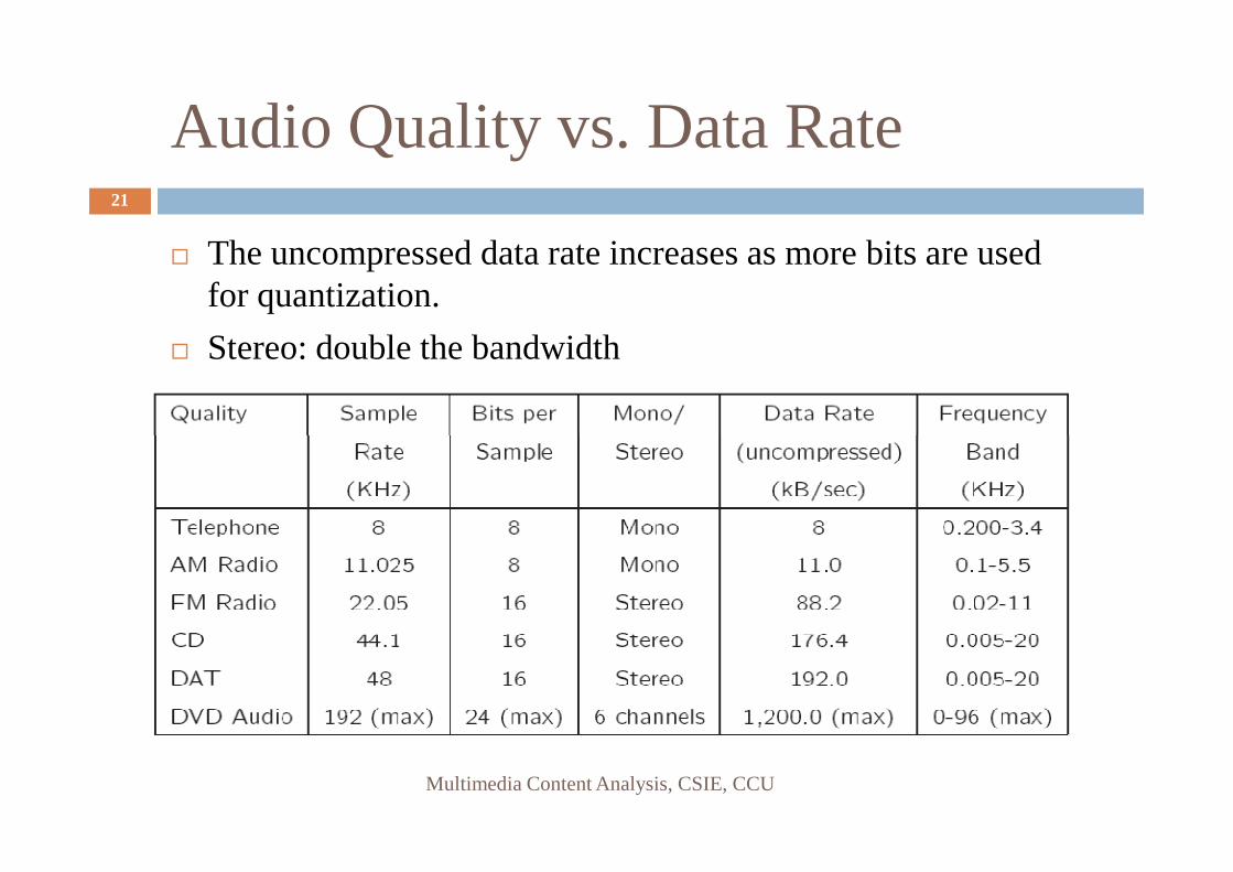
Audio Quality vs. Data Rate21
� The uncompressed data rate increases as more bits are used for quantization.
� Stereo: double the bandwidth
Multimedia Content Analysis, CSIE, CCU
Processing in Frequency Domain22
� It’s hard to infer much from the time-domain waveform.
� Human hearing is based on frequency analysis.
� Use of frequency analysis often facilitates
Multimedia Content Analysis, CSIE, CCU
� Use of frequency analysis often facilitates understanding.
Part of slides are from Prof. Hsu, NTUhttp://www.csie.ntu.edu.tw/~winston/courses/mm.ana.idx/index.html
Problems in Using Fourier Transform23
� Fourier transformation contains only frequency information
� No Time information is retained
� Works fine for stationary signals
Multimedia Content Analysis, CSIE, CCU
� Works fine for stationary signals
� Non-stationary or changing signals cause problems� Fourier transformation shows frequencies occurring at
all times instead of specific times

Short-Time Fourier Transform (STFT)24
� How can we still use FT, but handle nonstationarysignals?
� How can we include time?
� Idea: Break up the signal into discrete windows
Multimedia Content Analysis, CSIE, CCU
� Idea: Break up the signal into discrete windows
� Each signal within a window is a stationary signal
� Take FT over each part

STFT Example25
Multimedia Content Analysis, CSIE, CCU
Window function

Short-Time Fourier Analysis26
� Problem: Conventional Fourier analysis does not capture time-varying nature of audio signals
� Solution: Multiply signals by finite-duration
Multimedia Content Analysis, CSIE, CCU
� Solution: Multiply signals by finite-duration window function, then compute DTFT:
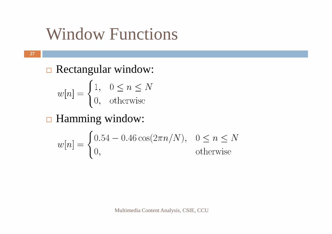
Window Functions27
� Rectangular window:
� Hamming window:
Multimedia Content Analysis, CSIE, CCU
� Hamming window:

Window Functions28
Multimedia Content Analysis, CSIE, CCU
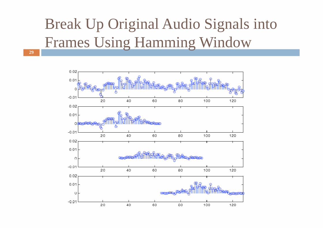
Break Up Original Audio Signals into Frames Using Hamming Window
29
Multimedia Content Analysis, CSIE, CCU
Wei-Ta Chu
Introduction of Audio Features30
2010/11/25
Multimedia Content Analysis, CSIE, CCU

Introduction of Audio Features31
� Short-term frame level vs. long-term clip level� A frame is defined as a group of neighboring samples which last about
10 to 40 ms� For audio clips with sampling frequency 16kHz, how many samples are in a
20ms audio frame?
Within an audio frame we can assume that the audio signal is stationary.
Multimedia Content Analysis, CSIE, CCU
� Within an audio frame we can assume that the audio signal is stationary.
� A clip consists of a sequence of frames, and clip-level features usually characterize how frame-level features change over a clip.
Y. Wang, Z. Liu, and J.-C. Huang, “Multimedia content analysis – using both audio and visual clues,” IEEE Signal Processing Magazine, Nov., 2000, pp. 12-36.

Frames and Clips32
� Fixed length clips (1 to 2 seconds) or vary-length clips
� Both frames and clips may overlap with their previous ones
Multimedia Content Analysis, CSIE, CCU

Frame-Level Features33
� Most of the frame-level features are inherited from speech signal processing.
� Time-domain features
� Frequency-domain features
Multimedia Content Analysis, CSIE, CCU
� Frequency-domain features
� We use N to denote the frame length, and sn(i) to denote the ith sample in the nth audio frame.
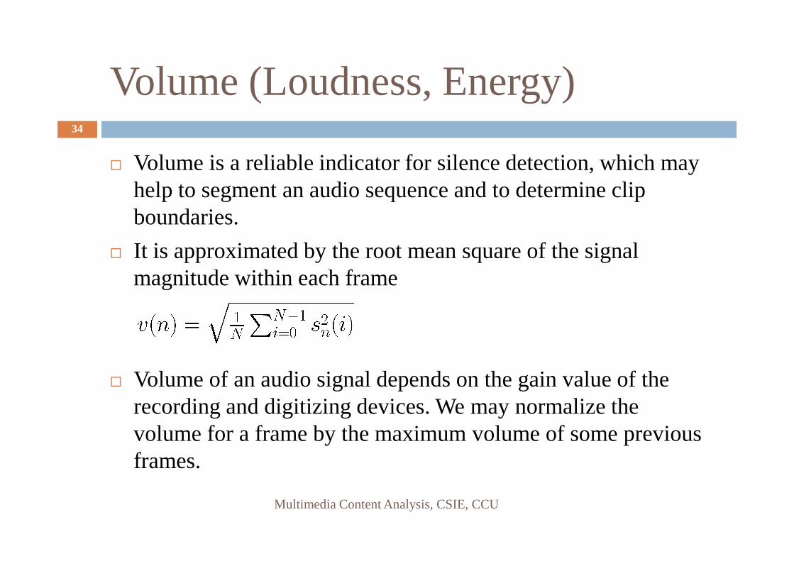
Volume (Loudness, Energy)34
� Volume is a reliable indicator for silence detection, which may help to segment an audio sequence and to determine clip boundaries.
� It is approximated by the root mean square of the signal magnitude within each frame
Multimedia Content Analysis, CSIE, CCU
magnitude within each frame
� Volume of an audio signal depends on the gain value of the recording and digitizing devices. We may normalize the volume for a frame by the maximum volume of some previous frames.

Zero Crossing Rate35
� Count the number of times that the audio waveform crosses the zero axis.
ZCR is one of the most indicative and robust measures to ZCR = the number of zero crossings per second
Multimedia Content Analysis, CSIE, CCU
� ZCR is one of the most indicative and robust measures to discern unvoiced speech. Typically, unvoiced speech has a low volume but a high ZCR.
� Using ZCR and volume together, one can prevent low energy unvoiced speech frames from being classified as silent.
Pitch36
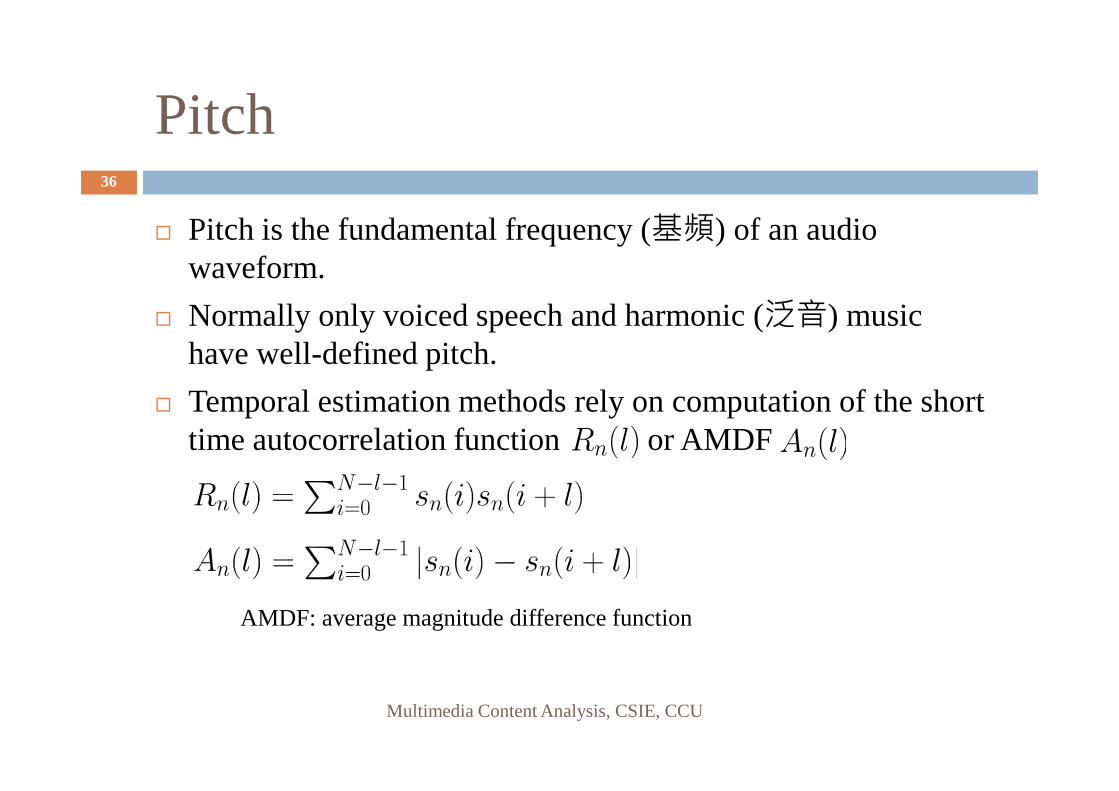
� Pitch is the fundamental frequency (基頻) of an audio waveform.
� Normally only voiced speech and harmonic (泛音) music have well-defined pitch.
� Temporal estimation methods rely on computation of the short
Multimedia Content Analysis, CSIE, CCU
� Temporal estimation methods rely on computation of the short time autocorrelation function or AMDF
AMDF: average magnitude difference function

Pitch37
� Valleys exist in voiced and music frames and vanish in noise and unvoiced frames.
Multimedia Content Analysis, CSIE, CCU
Spectral Features38
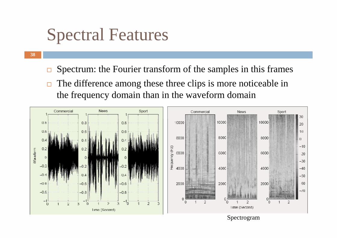
� Spectrum: the Fourier transform of the samples in this frames
� The difference among these three clips is more noticeable in the frequency domain than in the waveform domain
Spectrogram

Spectral Features39
� Let denote the power spectrum (i.e. magnitude square of the spectrum) of frame n.
� If we think of as a random variable and normalized by the total power as the probability density function of , we can define mean and standard deviation of .
Multimedia Content Analysis, CSIE, CCU
define mean and standard deviation of .
Frequency centroid, brightness
Bandwidth

SubbandEnergy Ratio40
� The ratio of the energy in a frequency subband to the total energy
� When the sampling rate is 22050 Hz, the frequency ranges for the four subbands are 0-630 Hz, 630-1720 Hz, 1720-4400 Hz, and 4400-11025 Hz.
Z. Liu, Y. Wang, and T. Chen, “Audio feature extraction and analysis for scene segmentation and classification,” Journal of VLSI Signal Processing, vol. 20, 1998, pp. 61-79.

Spectral Flux41
� Spectrum flux (SF) is defined as the average variation value of spectrum between the adjacent two frames.
� The SF values of speech are higher than those of music. The SF values of speech are higher than those of music.
� The environment sound is among the highest and changes more dramatically than the other two types of signal.
L. Lu, H.-J. Zhang, H. Jiang, “Content analysis for audio classification and segmentation,” IEEE Trans. on Speech and Audio Processing, vol. 10, no. 7, 2002, pp. 504-516.

Spectral Rolloff42
� The 95th percentile of the power spectral distribution.
� This measure distinguishes voiced from unvoiced speech. The value is higher for right-skewed distributions.
Multimedia Content Analysis, CSIE, CCU
distributions.� Unvoiced speech has a high proportion of energy contained
in the high-frequency range of the spectrum
� This is a measure of the “skewness” of the spectral shape
E. Scheirer and M. Slaney, “Construction and evaluation of a robust multifeatures speech/music discriminator,” Proc. of ICASSP, vol. 2, 1997, pp. 3741-3744.

MFCC (Mel-Frequency CepstralCoefficients)
43
� The most popular features in speech/audio/music processing.
� Segment incoming waveform into frames� Compute frequency response for each frame using
DFTs
Multimedia Content Analysis, CSIE, CCU
DFTs� Group magnitude of frequency response into 25-40
channels using triangular weighting functions� Compute log of weighted magnitudes for each channel� Take inverse DCT/DFT of weighted magnitudes for
each channel, producing ~14 cepstral coefficients for each frame
Par of slides are from Prof. Hsu, NTUhttp://www.csie.ntu.edu.tw/~winston/courses/mm.ana.idx/index.html
The Mel Weighting Functions44
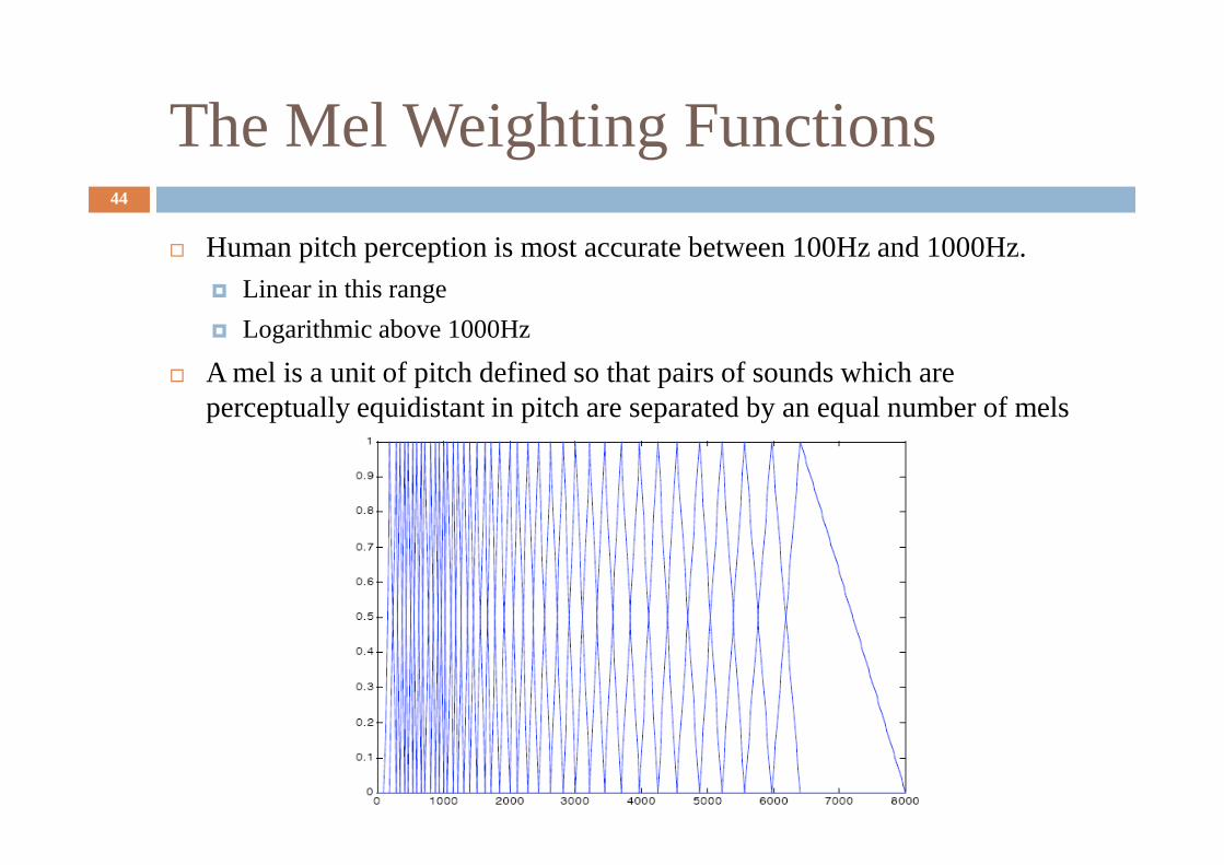
� Human pitch perception is most accurate between 100Hz and 1000Hz.
� Linear in this range
� Logarithmic above 1000Hz
� A mel is a unit of pitch defined so that pairs of sounds which are perceptually equidistant in pitch are separated by an equal number of mels
Multimedia Content Analysis, CSIE, CCU
Clip-Level Features45
� To extract the semantic content, we need to observe the temporal variation of frame features on a longer time scale.
� Volume-based features: � VSTD (volume standard deviation)
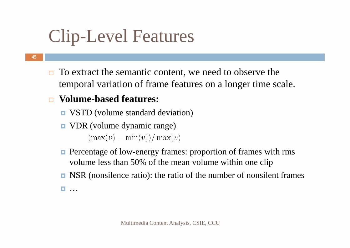
� VDR (volume dynamic range)
Multimedia Content Analysis, CSIE, CCU
� VDR (volume dynamic range)
� Percentage of low-energy frames: proportion of frames with rmsvolume less than 50% of the mean volume within one clip
� NSR (nonsilence ratio): the ratio of the number of nonsilent frames
� …

Clip-Level Features46
� ZCR-based features:� With a speech signal, low and high
ZCR periods interlaced. � ZSTD (standard deviation of ZCR)� Standard deviation of first order
differencedifference� Third central moment about the
mean� Total number of zero crossing
exceeding a threshold� Difference between the number of
zero crossings above and below the mean values
J. Saunders, “Real-time discrimination of broadcast speech/music,” Proc. of ICASSP, vol. 2, 1996, pp. 993-996.

Clip-Level Features47
� Pitch-based features: � PSTD (standard deviation of
pitch)� SPR (smooth pitch ratio): the
percentage of frames in a clip that have similar pitch as the that have similar pitch as the previous frames� Measure the percentage of
voiced or music frames within a clip
� NPR (nonpitch ratio): percentage of frames without pitch. � Measure how many frames are
unvoiced speech or noise within a clip
Wei-Ta Chu
Audio Segmentation and Classification48
2010/11/25
Multimedia Content Analysis, CSIE, CCU
T. Zhang and C.-C. J. Kuo, “Audio content analysis for online audiovisual data segmentation and classification,” IEEE Trans. on Speech and Audio Processing, vol. 9, no. 4, 2001, pp. 441-457.

Overview49
Multimedia Content Analysis, CSIE, CCU

Characteristics50
� 1. Taking into account hybrid types of sound which contain more than one kind of audio component.
� 2. Put more emphasis on the distinction of environmental sounds� Essential in many applications such as the post-processing of films
Multimedia Content Analysis, CSIE, CCU
� Essential in many applications such as the post-processing of films
� 3. Integrated features are exploited for audio classification
� 4. Low complexity
� 5. The proposed method is generic and model-free. � Used as the tool for segmentation and indexing of radio and TV
programs
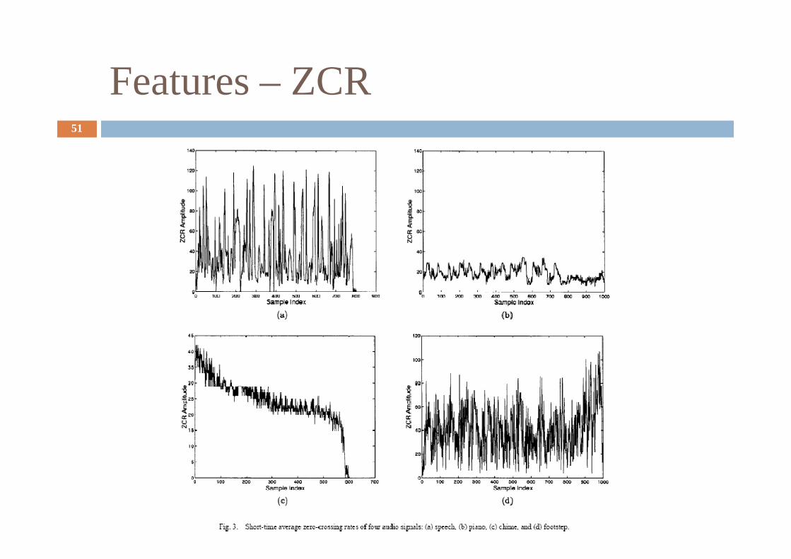
Features – ZCR 51
Multimedia Content Analysis, CSIE, CCU

Features – Fundamental Frequency52
� Distinguish between harmonic from nonharmonic sounds.
� Sounds from most musical instruments are harmonic.
� Speech signal is a harmonic and nonharmonic mixed sound.
� Most environmental sounds are nonharmonic.
Multimedia Content Analysis, CSIE, CCU

Features – Fundamental Frequency53
� All maxima in the spectrum are detected as potential harmonic peaks.
� Check among locations of peaks whether they have sharpness, amplitude, and width values satisfying certain criteria.
� If all conditions are met, the SFuF(short-time fundamental
Multimedia Content Analysis, CSIE, CCU
� If all conditions are met, the SFuF(short-time fundamental frequency) value is estimated as the frequency corresponding to the greatest common divider of locations of harmonic peaks; otherwise, SFuF is set to zero.

Features – Fundamental Frequency54
Multimedia Content Analysis, CSIE, CCU
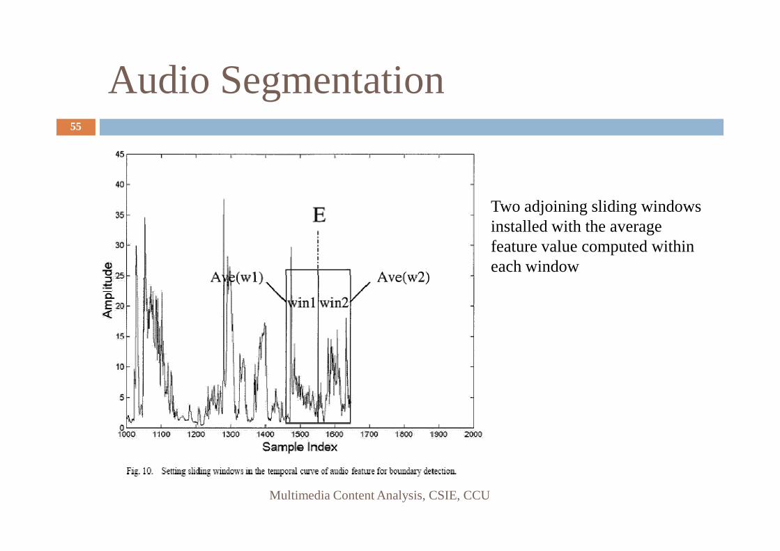
Audio Segmentation55
Two adjoining sliding windows installed with the average feature value computed within each window
Multimedia Content Analysis, CSIE, CCU
each window
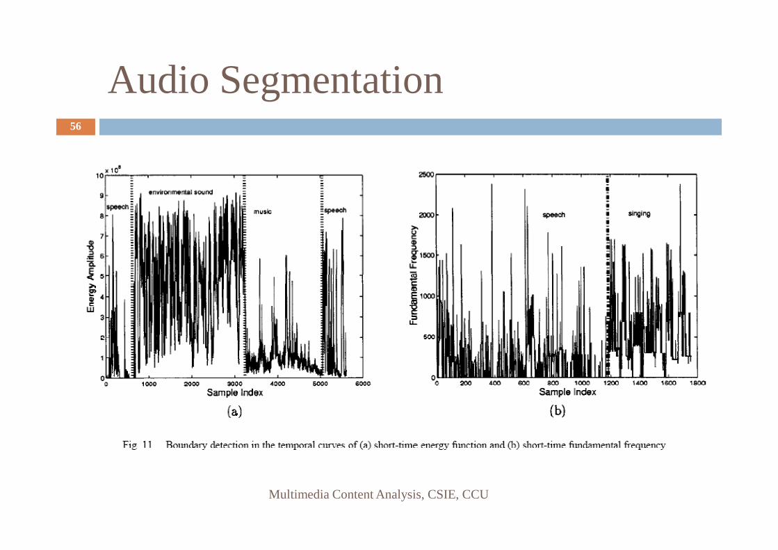
Audio Segmentation56
Multimedia Content Analysis, CSIE, CCU

Audio Classification57
� 1. Detecting silence: � If the short-time energy is continuously lower than a
threshold, or if most short-time average ZCR is lower than a threshold
2. Separating sounds with/without music components
Multimedia Content Analysis, CSIE, CCU
� 2. Separating sounds with/without music components� By detecting continuous and stable frequency peaks from
the power spectrum
� Based on a threshold for the zero ratio at about 0.7
� > 0.7: pure speech or nonharmonic environmental sound
� <0.7: otherwise
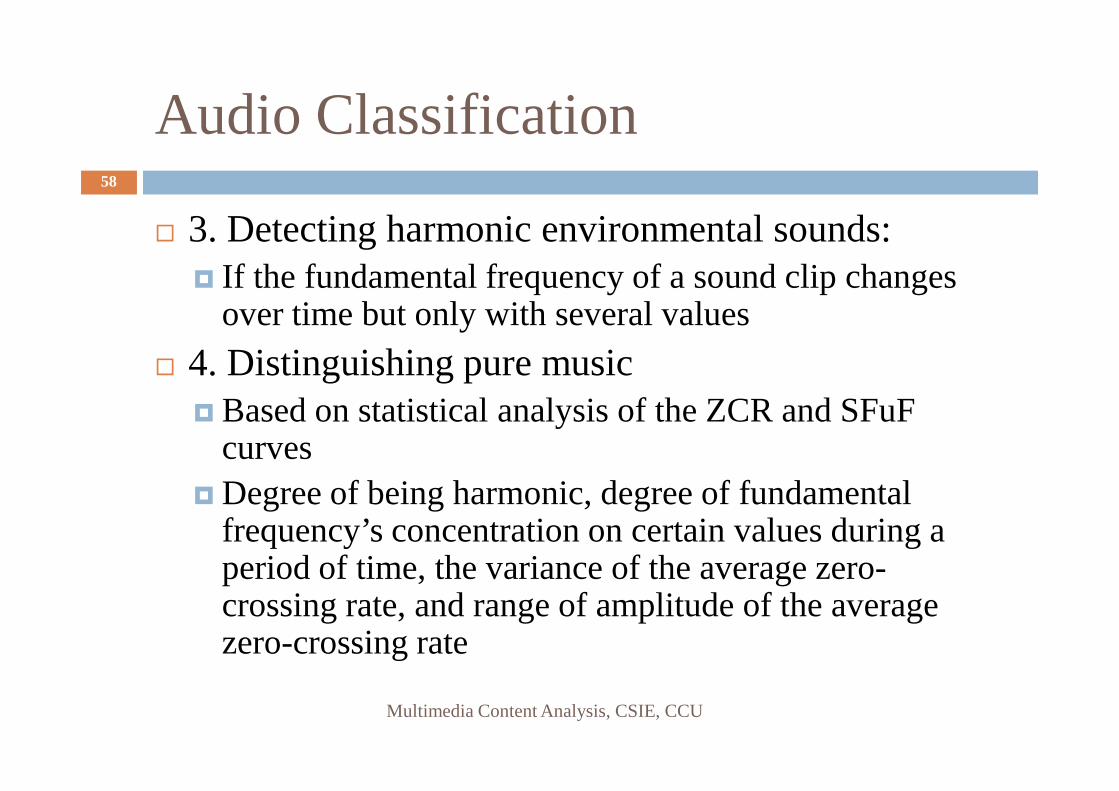
Audio Classification58
� 3. Detecting harmonic environmental sounds: � If the fundamental frequency of a sound clip changes
over time but only with several values
� 4. Distinguishing pure musicBased on statistical analysis of the ZCR and SFuF
Multimedia Content Analysis, CSIE, CCU
� Based on statistical analysis of the ZCR and SFuFcurves
� Degree of being harmonic, degree of fundamental frequency’s concentration on certain values during a period of time, the variance of the average zero-crossing rate, and range of amplitude of the average zero-crossing rate

Audio Classification59
� 5. Distinguishing songs
� 6. Separating speech/environmental sound with music background
� 7. Distinguish pure speech
Multimedia Content Analysis, CSIE, CCU
� 7. Distinguish pure speech
� 8. Classifying Nonharmonic environmental sounds
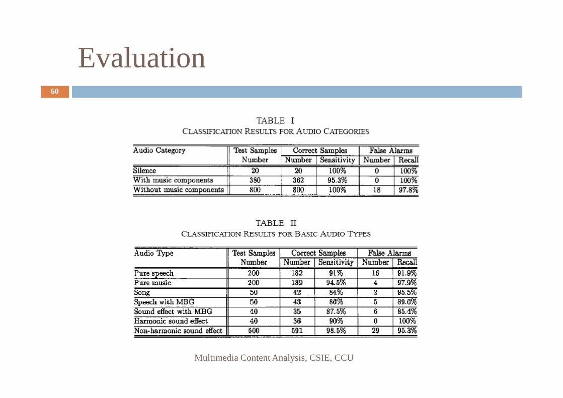
Evaluation60
Multimedia Content Analysis, CSIE, CCU
References61
� Y. Wang, Z. Liu, and J.-C. Huang, “Multimedia content analysis – using both audio and visual clues,” IEEE Signal Processing Magazine, Nov., 2000, pp. 12-36. (must read)
� Z. Liu, Y. Wang, and T. Chen, “Audio feature extraction and analysis for scene segmentation and classification,” Journal of
Multimedia Content Analysis, CSIE, CCU
analysis for scene segmentation and classification,” Journal of VLSI Signal Processing, vol. 20, 1998, pp. 61-79.
� T. Zhang and C.-C. J. Kuo, “Audio content analysis for online audiovisual data segmentation and classification,” IEEE Trans. on Speech and Audio Processing, vol. 9, no. 4, 2001, pp. 441-457.

![Welcome [] · 230 - 249 anglican high school catholic high school chij katong convent chung cheng high school (main) dunman sec school chung cheng high school (main) maris stella](https://img.pdfslide.us/doc/110x75/5e7761b1101d427ecf47fe4a/welcome-230-249-anglican-high-school-catholic-high-school-chij-katong-convent.jpg)