POLYMERSCesar Beleno, Kaven Yau

Computational Physics Project, Universitat Bonn, WS 10/11

ABSTRACT

In this report we present the results of the simulation of polymers in the athermal limit;

that is, the polymer chain is immersed in a good solvent. For that purpose static and

dynamic random walk generation methods were considered. Within the static methods

we implemented the simple and biased sampling; while among the dynamic methods, we

used reptation, kink-jump and pivot algorithm. For each case, the algorithm efficiency

was analyzed, the end-to-end distance was obtained, and a value for the fractal dimension

was obtained for each case. A description of each algorithm is also included.

1 Introduction

A polymer is a macromolecule composed of repeating structural units (monomers), typically connectedby covalent chemical bonds. It can be modeled as a very large chain of N monomers, with N being ofthe order of 103 - 105. Their typical length ranges from 10−5 to 10−2 cm, although they are not widerthan 10−7 cm. They can be found in a range of materials, from textile fibers, plastics, rubber, andcellulose, to the proteins in living organisms[1].

Although the chemical properties of the polymers can be described well by chemical formulas, theirphysical properties are strongly related to their geometry. A characteristic example is the distancebetween one end and the other end of the polymer, which characterizes the behavior of a polymersubmerged in a chemical solution. From the literature, it is known that for a diluted solution ofpolymer chains the dependence of this quantity to the number of monomers in the chain is given byeq.1:

〈R2N 〉 = aN2ν (1)

where the proportionality constant a depends on the structure and on the solvent used in the chemicalsolution. For two dimensions (2d) the value for the parameter ν is 3/4, for three dimensions (3d) it isapproximately 0.592 and for 4 dimensions (4d) it is 1/2 [2].

The numerical simulation in this study will focus on linear polymers in a liquid solvent. Sinceonly a small fraction of the space containing the solution is actually occupied by the polymer chain,the remaining space is assumed to be filled with the solvent molecules. The interactions present inthis kind of system can be classified as between monomers, between solvent molecules, and betweensolvent molecules and monomers. These interactions can be well described by the Lennard-Jonesinteraction, which is strongly repulsive at short distances and weakly attractive at longer distances.As the repulsive part dominates, there is a more simplified approach, known as excluded volumeinteraction, which basically states that two monomers cannot occupy the same spatial position[3].

2 Self-avoiding walks (SAW) and Polymer chains

Let’s consider a d-dimensional lattice. A self-avoiding walk (SAW) is a sequence of distinct points inthe lattice such that each point is a nearest neighbor of its predecessor. The SAW model is well-knownfor polymer molecules[7].

In a d-dimensional (hyper)cubic lattice subject to unitary steps constrain, there are 2d step choicesavailable for each site. By adding the constrain that each step remembers locally the former step, so itis not allowed to step backwards, one choice is removed. Therefore, at any given site, there are 2d− 1choices. The only exception is the first step, where all 2d choices are available1.

1Usually the first step can be chosen arbitrarily due to symmetry considerations. Therefore, this exception is irrelevant.

1

Generally, we are interested in the average of certain quantities such as the end-to-end distance.For a given walk size, the average, the standard deviation, and the relative error are computed usingstandard statistics. In the case of end-to-end distance quantity, the relative error approaches a constantand therefore it can be used as a test for randomness in the algorithm.

The partition function that provides information about the efficiency of generation of chains oflength N can be written as:

〈Z(N)〉ss =number of accepted walks

number of attempts(2)

If each walk has a different weight W , the weight has to be taken into account. For the standarddeviation, it is more convenient to use the following expression2:

σX =√〈X2〉 − 〈X〉2 (3)

And for the partition function[5]:

Zbs =

∑all walks Wwalk

number of attempts= 〈W 〉 (4)

In both the simple and biased sampling the partition function present the following form:

ZN = C exp(−λN)Nγ−1 (5)

where C is a normalization constant, λ is a model dependent constant called the attrition constant,and γ is a critical exponent that is independent of the model. Another quantity that accounts for thefluctuation of the end-to-end distance es the relative variance given by:

∆R2 =

√〈R4〉 − 〈R2〉2

〈R2〉(6)

This quantity tends to a constant due to the lack of self-averaging of the end-to-end distance [4].

3 Model and Algorithms

Among all the existing polymer models, we will restrict ourselves to d-dimensional (hyper)cubic lattices.From here on, we will use the word lattice to refer to a (hyper)cubic lattice.

In our analysis, a flexible polymer chain in a periodic lattice is replaced by a randomly generatedSAW. As there are many methods to randomly generate a SAW, the algorithms used in this study arelisted, explained, and discussed in this section.

3.1 Static methods

Static methods generate a sequence of statistically independent samples. In other words, each iterationis independent of former iterations[7]. The static methods used in this study are the simple samplingand the Rosenbluth method.

3.1.1 Simple Sampling

The simple sampling is, as the name indicates, a quite uncomplicated method. The steps are generatedrandomly, with the only constrain that each step remembers locally the former step, so it is not allowedto step backwards. For a d-dimensional lattice, the algorithm is the following[4]:

2The weighted average formula is omitted, but it can be found in most basic statistic books.

2

i. Set the origin of the polymer. In our study, we set it at the coordinate system’s origin.

ii. Generate the first step randomly or choose it arbitrarily.

iii. Choose randomly one of the 2d− 1 possible steps.

iv. If the step leads to self-intersection, reject the generated walk and start over again. This step isneeded to ensure randomness.

v. If the step leads to an available site, add the step to the walk.

vi. If the walk reaches the wanted length, accept the walk. Else, go to step iii and repeat until thewalk is either accepted or rejected.

vii. Repeat until the wanted walks amount is reached.

Advantages:

• It is easy to program in a computer.

• the method is intuitive.

• The algorithm has no bias and all possible configurations can be reached.

Disadvantages:

• The algorithm efficiency decreases very fast as the walk size increases. For very long polymerchains, the low efficiency becomes prohibitive.

3.2 Biased sampling

The biased sampling 3 is an improved simple sampling method. The main problem of the simplesampling is that at large walk sizes and small dimensions the rejection rate is very high. In order toreduce the rejection rate, the steps that lead to self-intersection are excluded in step iii [5].

To correct for the bias that is introduced by the exclusion of those steps, a weight W is assigned toeach walk, based on how many steps were excluded. The weight for a walk size N, in a n-dimensionallattice is given by:

W =N∏i=1

wi (7)

where wi are the partial weights for each step and are defined as:

w0 = 1 (8)

wi =li

2d− 1(9)

where li is the number of available steps from where the i-th step was chosen. Note that if there areno available steps, the weight becomes 0 and the walk is rejected. Summarizing, for a d-dimensionallattice, the Rosenbluth method algorithm can be implemented as follows [2]:

i. Set the origin of the polymer. In our study, we set it at the coordinate system’s origin.

ii. Generate the first step randomly or choose it arbitrarily.

3Also called Rosenbluth method

3

iii. Find all possible steps that do not lead to self-intersection.

iv. If no steps are available, set the weight to 0, reject the generated walk, and start over again. Else,add the step to the walk and compute the partial weight using equation (9).

v. If the walk reaches the wanted length, accept the walk and compute the total weight using equation(7). Else, go to step iii and repeat until the walk is either accepted or rejected.

vi. Repeat until the wanted walks amount is reached.

Advantages:

• It offers a significant improvement to the efficiency compared to the simple sampling.

• The method is still intuitive and relatively easy to program.

• The algorithm has no bias and all possible configurations can be reached.

Disadvantages:

• Although the efficiency is better than the simple sampling efficiency, it still decreases very fastas the walk size increases. For very long polymer chains, the low efficiency becomes prohibitive.

3.3 Dynamic methods

Dynamic methods generate a sequence of correlated samples. In other words, each iteration dependson at least the last iteration[7]. The dynamic methods we used are the reptation, kink-jump and pivotalgorithms. All these algorithms are Markov chains, that is, the new configuration depends only onthe last configuration[8].

3.3.1 Reptation algorithm

This is one of the most efficient generation techniques and is applicable to any linear polymer chainmodel. The algorithm can be stated as follows[2, 6] 4:

i. Generate or choose a n-steps SAW.

ii. Choose an end randomly and remove this site.

iii. Choose randomly one of the 2d− 1 possible steps on the other end.

iv. If the attempt leads to self-intersection, retain the previous configuration and count it as the newconfiguration.

v. If the attempt does not lead to self-intersection, count it as the new configuration.

vi. Go to step ii and repeat until the wanted walks amount is reached.

Advantages:

• The method is very efficient.

• Each iteration requires little computational work.

4Other algorithms for the reptation method exist

4

Disadvantages:

• The method is not intuitive.

• The algorithm is somewhat sensitive to the initial condition.

• The results are biased: There are some configurations that we will never obtain, such as doubleended ”cul-de-sac” configurations (figure). In this way, the reptation method includes a smallbias that can be neglected with sufficient statistics.

3.3.2 Kink-Jump algorithm

This model is used to simulate the dynamics of the collisions between the polymer chain and thesolvent molecules. For that purpose, the chain is assumed to be composed of beads connected bybonds, whose motion is restricted to a lattice. The algorithm can be described as follows[2]:

i. Generate or choose a n-steps SAW.

ii. Select a bead (occupied site) at random on the walk.

iii. If the bead is not the head or the tail, then the bead can move to only one site without breakingthe walk continuity. If this site is not occupied, move the selected bead there. Otherwise, keepthe current walk.

iv. If the selected bead is the head or the tail, move it to one of the two (maximum) possible unoccupiedsites so that the bond to which it is connected changes its orientation by ±90. If no sites areavailable, keep the current walk.

v. Count the walk.

vi. Go to step ii and repeat until the wanted walks amount is reached.

Advantages:

• Each iteration requires little computational work.

• It simulates the dynamics of the collisions between the polymer chain and molecules.

Disadvantages:

• The results are biased: there are some configurations that we will never obtain, such as doubleended ”cul-de-sac” configurations (figure).

• The algorithm is highly sensitive to the initial condition. This means that it requires manyiterations before given a configuration reaches an essentially new configuration.

• the algorithm is biased, favouring longer chains.

3.3.3 Pivot algorithm

The pivot algorithm generates SAWs from an initial SAW. At each iteration, the SAW from the lastiteration is modified by randomly choosing a pivot bead and randomly applying one lattice symmetryoperation on one of the two sub-walks. The new SAWs will always have the same number of steps asthe initial SAW. The algorithm can be sketched as follows[7]:

i. Generate or choose a n-steps SAW.

5

ii. Randomly choose a pivot from the beads on the walk. The walk can be then divided in twosub-walks joined by the pivot.

iii. Randomly choose one of the two sub-walks.

iv. Randomly choose a lattice symmetry operation and apply it to the chosen sub-walk.

v. If the attempt violates the self-intersection constraint, retain the previous configuration and countit as the new configuration.

vi. If the attempt does not break the self-intersection constrain, count it as the new configuration.

vii. Go to step ii and repeat until the wanted walks amount is reached.

Advantages:

• Fast convergence: after a few iterations, a configuration can be considered to have reached anessentially new configuration.

• The algorithm is unbiased and all possible configurations can be reached.

Disadvantages:

• Each iteration requires more computational work than the other two dynamical methods.

• Its implementation in a computer program is difficult for high dimensions: the number of sym-metries increases very fast and the symmetry operations are difficult to compute.

• For long polymer chains, the efficiency is very low. But this is compensated with a fast conver-gence.

4 Numerical Results and Analysis

4.1 Static Algorithms

4.1.1 Simple Sampling

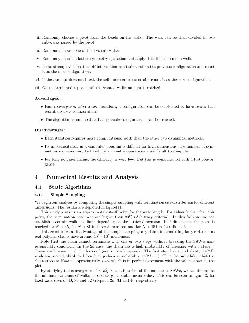
We begin our analysis by computing the simple sampling walk termination size distribution for differentdimensions. The results are depicted in figure(1).

This study gives us an approximate cut-off point for the walk length. For values higher than thispoint, the termination rate becomes higher than 99% (Arbitrary criteria). In this fashion, we canestablish a certain walk size limit depending on the lattice dimension. In 2 dimensions the point isreached for N > 45, for N > 81 in three dimensions and for N > 151 in four dimensions.

This constitutes a disadvantage of the simple sampling algorithm in simulating longer chains, asreal polymer chains have around 103 - 105 monomers.

Note that the chain cannot terminate with one or two steps without breaking the SAW’s non-reversibility condition. In the 2d case, the chain has a high probability of breaking with 3 steps 5.There are 8 ways in which this configuration could appear. The first step has a probability 1/(2d),while the second, third, and fourth steps have a probability 1/(2d− 1). Thus the probability that thechain stops at N=3 is approximately 7.4% which is in perfect agreement with the value shown in theplot.

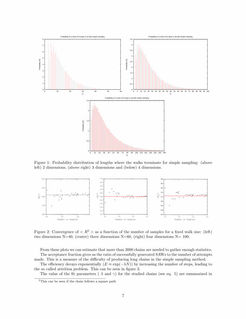
By studying the convergence of < R2N > as a function of the number of SAWs, we can determine

the minimum amount of walks needed to get a stable mean value. This can be seen in figure 2, forfixed walk sizes of 40, 80 and 120 steps in 2d, 3d and 4d respectively.

6

0

1

2

3

4

5

6

7

8

0 10 20 30 40 50 60

Pro

babi

lity

[%]

N

Probability of a chain of N steps in 2d with simple sampling

0

0.5

1

1.5

2

2.5

3

3.5

4

4.5

0 5 10 15 20 25 30 35 40 45 50 55 60 65 70 75 80 85 90 95 100

Pro

babi

lity

[%]

N

Probability of a chain of N steps in 3d with simple sampling

0

0.5

1

1.5

2

2.5

0 10 20 30 40 50 60 70 80 90 100 110 120 130 140 150 160

Pro

babi

lity

[%]

N

Probability of a chain of N steps in 4d with simple sampling

Figure 1: Probability distribution of lengths where the walks terminate for simple sampling: (aboveleft) 2 dimensions, (above right) 3 dimensions and (below) 4 dimensions.

102 103 104180

190

200

210

220

<RN2 >

Number of Samples

102 103 104 105120125130135140145150155160165170

<RN2 >

Number of Samples

102 103 104 105150

155

160

165

170

175

180

185

190

<RN2 >

Number of Samples

Figure 2: Convergence of < R2 > as a function of the number of samples for a fixed walk size: (left)two dimensions N=40, (center) three dimensions N=60, (right) four dimensions N= 100.

From these plots we can estimate that more than 2000 chains are needed to gather enough statistics.The acceptance fraction gives us the ratio of successfully generated SAWs to the number of attempts

made. This is a measure of the difficulty of producing long chains in the simple sampling method.The efficiency decays exponentially (E ≈ exp(−λN)) by increasing the number of steps, leading to

the so called attrition problem. This can be seen in figure 3.The value of the fit parameters ( λ and γ) for the studied chains (see eq. 5) are summarized in

5This can be seen if the chain follows a square path

7

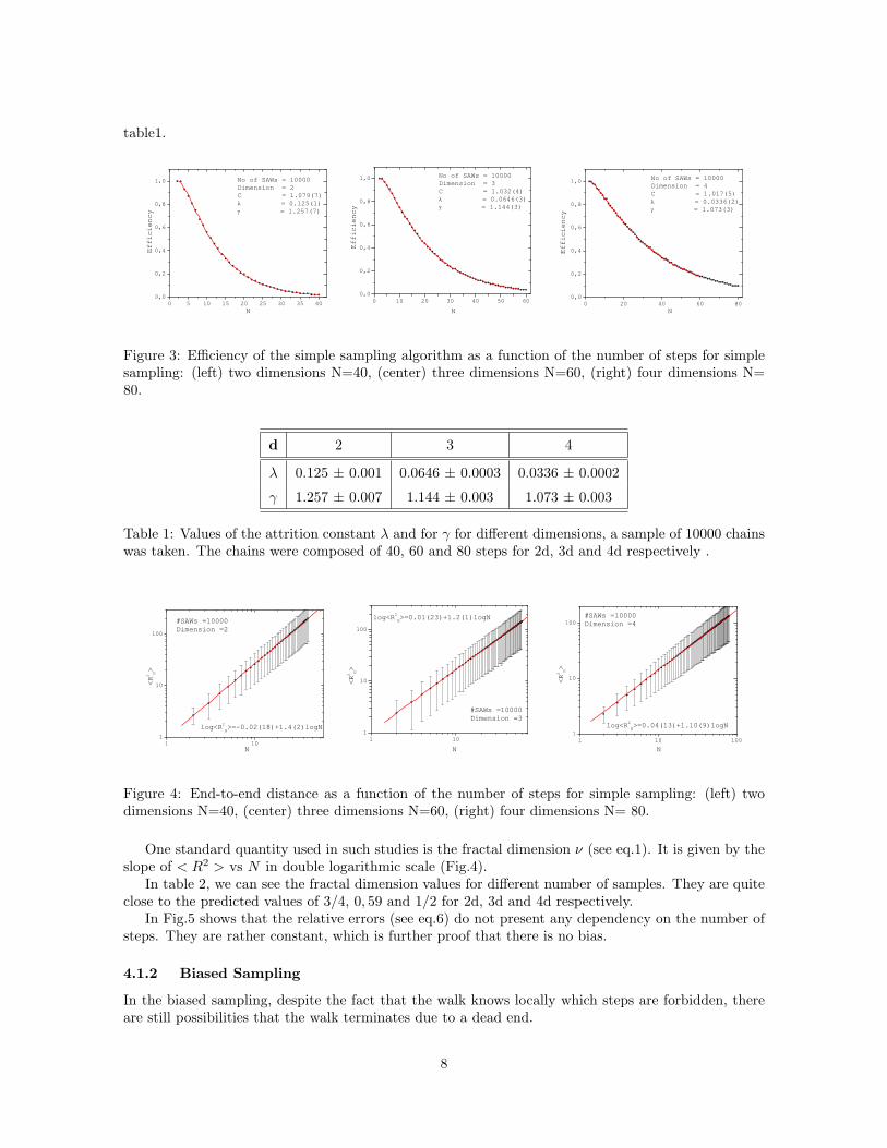
table1.

0 5 10 15 20 25 30 35 400,0

0,2

0,4

0,6

0,8

1,0 No of SAWs = 10000Dimension = 2C = 1.079(7) = 0.125(1) = 1.257(7)

N

Efficiency

0 10 20 30 40 50 600,0

0,2

0,4

0,6

0,8

1,0 No of SAWs = 10000Dimension = 3C = 1.032(4) = 0.0646(3) = 1.144(3)

N

Efficiency

0 20 40 60 800,0

0,2

0,4

0,6

0,8

1,0 No of SAWs = 10000Dimension = 4C = 1.017(5) = 0.0336(2) = 1.073(3)

Efficiency

N

Figure 3: Efficiency of the simple sampling algorithm as a function of the number of steps for simplesampling: (left) two dimensions N=40, (center) three dimensions N=60, (right) four dimensions N=80.

d 2 3 4

λ 0.125 ± 0.001 0.0646 ± 0.0003 0.0336 ± 0.0002

γ 1.257 ± 0.007 1.144 ± 0.003 1.073 ± 0.003

Table 1: Values of the attrition constant λ and for γ for different dimensions, a sample of 10000 chainswas taken. The chains were composed of 40, 60 and 80 steps for 2d, 3d and 4d respectively .

1 101

10

100

<R2 N>

log<R2N>=-0.02(18)+1.4(2)logN

#SAWs =10000Dimension =2

N

1 101

10

100log<R2

N>=0.01(23)+1.2(1)logN

#SAWs =10000Dimension =3

N

<R2 N>

1 10 1001

10

100

<R2 N>

N

log<R2N>=0.04(13)+1.10(9)logN

#SAWs =10000Dimension =4

Figure 4: End-to-end distance as a function of the number of steps for simple sampling: (left) twodimensions N=40, (center) three dimensions N=60, (right) four dimensions N= 80.

One standard quantity used in such studies is the fractal dimension ν (see eq.1). It is given by theslope of < R2 > vs N in double logarithmic scale (Fig.4).

In table 2, we can see the fractal dimension values for different number of samples. They are quiteclose to the predicted values of 3/4, 0, 59 and 1/2 for 2d, 3d and 4d respectively.

In Fig.5 shows that the relative errors (see eq.6) do not present any dependency on the number ofsteps. They are rather constant, which is further proof that there is no bias.

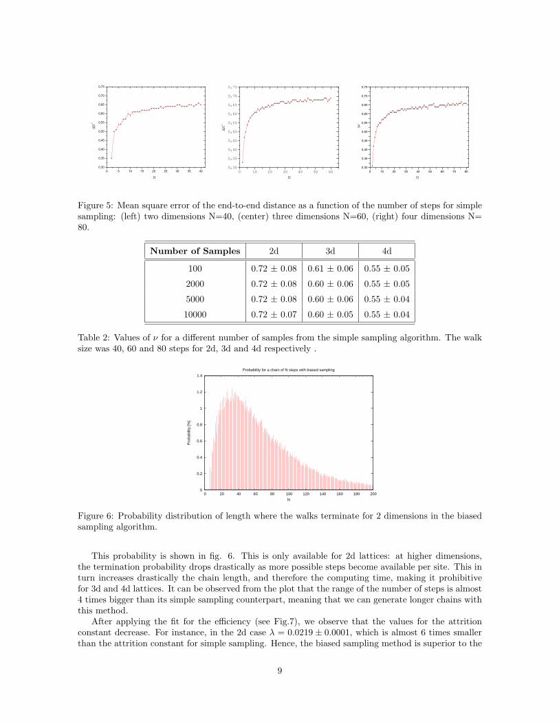
4.1.2 Biased Sampling

In the biased sampling, despite the fact that the walk knows locally which steps are forbidden, thereare still possibilities that the walk terminates due to a dead end.

8

0 5 10 15 20 25 30 35 400,30

0,35

0,40

0,45

0,50

0,55

0,60

0,65

0,70

0,75

N

R2

0 10 20 30 40 50 600,30

0,35

0,40

0,45

0,50

0,55

0,60

0,65

0,70

0,75

N

R2

0 10 20 30 40 50 60 70 800,30

0,35

0,40

0,45

0,50

0,55

0,60

0,65

0,70

0,75

R2

N

Figure 5: Mean square error of the end-to-end distance as a function of the number of steps for simplesampling: (left) two dimensions N=40, (center) three dimensions N=60, (right) four dimensions N=80.

Number of Samples 2d 3d 4d

100 0.72 ± 0.08 0.61 ± 0.06 0.55 ± 0.05

2000 0.72 ± 0.08 0.60 ± 0.06 0.55 ± 0.05

5000 0.72 ± 0.08 0.60 ± 0.06 0.55 ± 0.04

10000 0.72 ± 0.07 0.60 ± 0.05 0.55 ± 0.04

Table 2: Values of ν for a different number of samples from the simple sampling algorithm. The walksize was 40, 60 and 80 steps for 2d, 3d and 4d respectively .

0

0.2

0.4

0.6

0.8

1

1.2

1.4

0 20 40 60 80 100 120 140 160 180 200

Pro

babi

lity

[%]

N

Probability for a chain of N steps with biased sampling

Figure 6: Probability distribution of length where the walks terminate for 2 dimensions in the biasedsampling algorithm.

This probability is shown in fig. 6. This is only available for 2d lattices: at higher dimensions,the termination probability drops drastically as more possible steps become available per site. This inturn increases drastically the chain length, and therefore the computing time, making it prohibitivefor 3d and 4d lattices. It can be observed from the plot that the range of the number of steps is almost4 times bigger than its simple sampling counterpart, meaning that we can generate longer chains withthis method.

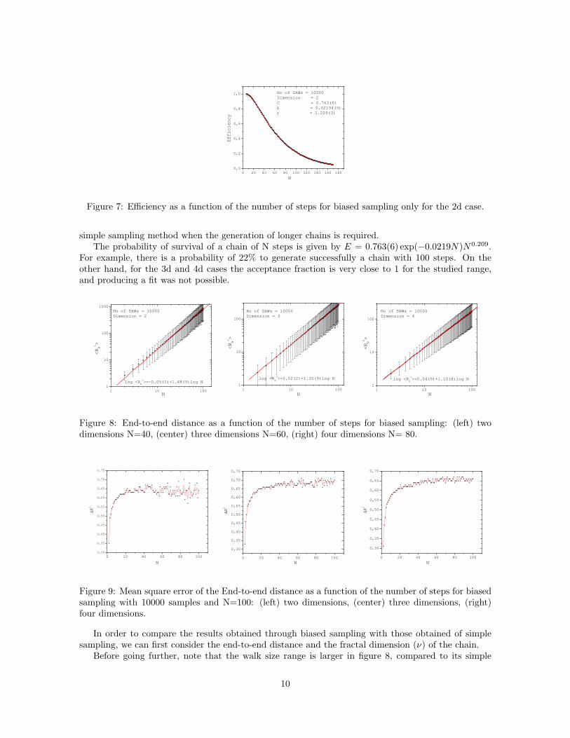
After applying the fit for the efficiency (see Fig.7), we observe that the values for the attritionconstant decrease. For instance, in the 2d case λ = 0.0219 ± 0.0001, which is almost 6 times smallerthan the attrition constant for simple sampling. Hence, the biased sampling method is superior to the

9

0 20 40 60 80 100 120 140 160 1800,0

0,2

0,4

0,6

0,8

1,0 No of SAWs = 10000Dimension = 2C = 0.763(6) = 0.02194(9) = 1.209(3)

N

Efficiency

Figure 7: Efficiency as a function of the number of steps for biased sampling only for the 2d case.

simple sampling method when the generation of longer chains is required.The probability of survival of a chain of N steps is given by E = 0.763(6) exp(−0.0219N)N0.209.

For example, there is a probability of 22% to generate successfully a chain with 100 steps. On theother hand, for the 3d and 4d cases the acceptance fraction is very close to 1 for the studied range,and producing a fit was not possible.

1 10 1001

10

100

1000

log <RN2>=-0.05(1)+1.48(9)log N

No of SAWs = 10000Dimension = 2

N

<RN2 >

1 10 1001

10

100

N

<RN2 >

No of SAWs = 10000Dimension = 3

log <RN2>=0.02(2)+1.20(9)log N

1 10 1001

10

100

log <RN2>=0.04(9)+1.10(8)log N

No of SAWs = 10000Dimension = 4

N

<RN2 >

Figure 8: End-to-end distance as a function of the number of steps for biased sampling: (left) twodimensions N=40, (center) three dimensions N=60, (right) four dimensions N= 80.

0 20 40 60 80 1000,30

0,35

0,40

0,45

0,50

0,55

0,60

0,65

0,70

0,75

N

R2

0 20 40 60 80 100

0,30

0,35

0,40

0,45

0,50

0,55

0,60

0,65

0,70

0,75

R2

N

0 20 40 60 80 100

0,30

0,35

0,40

0,45

0,50

0,55

0,60

0,65

0,70

N

R2

Figure 9: Mean square error of the End-to-end distance as a function of the number of steps for biasedsampling with 10000 samples and N=100: (left) two dimensions, (center) three dimensions, (right)four dimensions.

In order to compare the results obtained through biased sampling with those obtained of simplesampling, we can first consider the end-to-end distance and the fractal dimension (ν) of the chain.

Before going further, note that the walk size range is larger in figure 8, compared to its simple

10

sampling counterpart. Using the values for walk size and dimension used in the simple samplinganalysis. we fitted the value for ν. Additionally, we made the same analysis for 2d, 3d and 4d with awalk size of 100. The results of the fitting are arranged in table 3.

As observed, these results are in perfect agreement with the expected values. However, in the caseof the errors in the end-to-end distance, we can observe fluctuations around certain values (see Figure9).

Number of Samples 2d N=40 2d N=100 3d N=60 3d N=100 4d N=80 4d N=100

100 0.71 ± 0.07 0.73 ± 0.05 0.61 ± 0.06 0.60 ± 0.07 0.54 ± 0.05 0.54 ± 0.05

1000 0.72 ± 0.07 0.74 ± 0.05 0.60 ± 0.06 0.60 ± 0.05 0.54 ± 0.05 0.54 ± 0.04

10000 0.74 ± 0.04 0.74 ± 0.04 0.60 ± 0.05 0.60 ± 0.05 0.55 ± 0.04 0.55 ± 0.04

Table 3: Values of ν for different number of samples and walk size from the biased sampling algorithm.

4.2 Dynamic Algorithms

4.2.1 Reptation Method

0 20 40 60 80 100

0,70

0,75

0,80

0,85

0,90

0,95

1,00

Acceptance Fraction

N

No of SAWs = 50000Dimension = 2C = 0.96(1) = -0.0006(2) = 0.931(6)

0 20 40 60 80 1000,80

0,85

0,90

0,95

1,00 No of SAWs = 50000Dimension = 3C = 0.924(4) = -0.00038(3) = 0.976(1)

N

Acceptance Fraction

20 40 60 80 100

0,90

0,92

0,94

0,96

0,98

1,00

N

Acceptance Fraction

No of SAWs = 50000Dimension = 4C = 0.940(1) = -0.00020(2) = 0.9883(7)

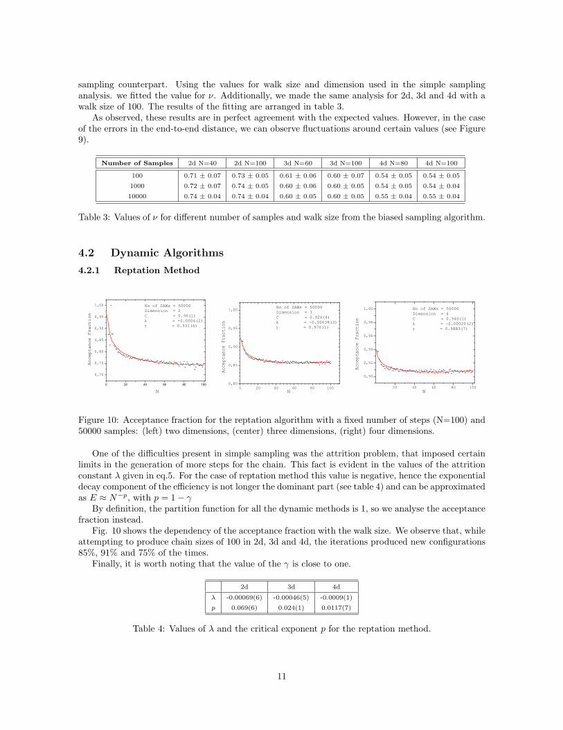
Figure 10: Acceptance fraction for the reptation algorithm with a fixed number of steps (N=100) and50000 samples: (left) two dimensions, (center) three dimensions, (right) four dimensions.

One of the difficulties present in simple sampling was the attrition problem, that imposed certainlimits in the generation of more steps for the chain. This fact is evident in the values of the attritionconstant λ given in eq.5. For the case of reptation method this value is negative, hence the exponentialdecay component of the efficiency is not longer the dominant part (see table 4) and can be approximatedas E ≈ N−p, with p = 1− γ

By definition, the partition function for all the dynamic methods is 1, so we analyse the acceptancefraction instead.

Fig. 10 shows the dependency of the acceptance fraction with the walk size. We observe that, whileattempting to produce chain sizes of 100 in 2d, 3d and 4d, the iterations produced new configurations85%, 91% and 75% of the times.

Finally, it is worth noting that the value of the γ is close to one.

2d 3d 4d

λ -0.00069(6) -0.00046(5) -0.0009(1)

p 0.069(6) 0.024(1) 0.0117(7)

Table 4: Values of λ and the critical exponent p for the reptation method.

11

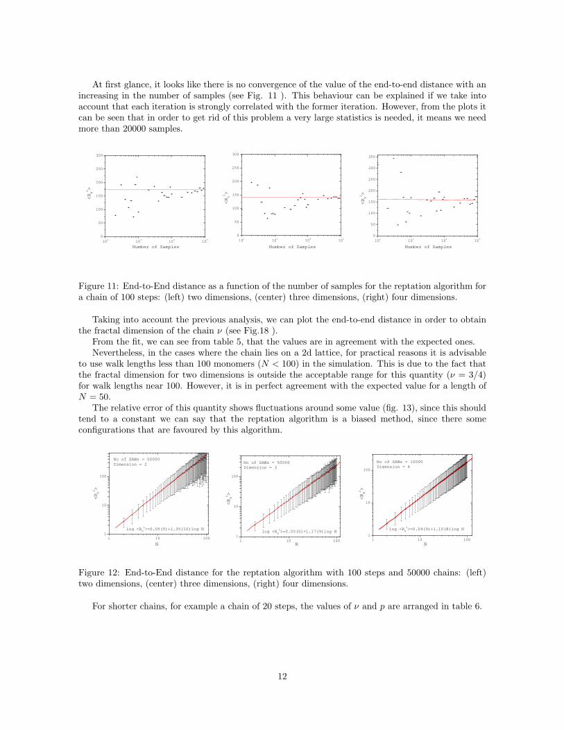
At first glance, it looks like there is no convergence of the value of the end-to-end distance with anincreasing in the number of samples (see Fig. 11 ). This behaviour can be explained if we take intoaccount that each iteration is strongly correlated with the former iteration. However, from the plots itcan be seen that in order to get rid of this problem a very large statistics is needed, it means we needmore than 20000 samples.

102 103 104 1050

50

100

150

200

250

300

Number of Samples

<RN2 >

102 103 104 1050

50

100

150

200

250

300

Number of Samples

<RN2 >

102 103 104 1050

50

100

150

200

250

300

350

Number of Samples

<RN2 >

Figure 11: End-to-End distance as a function of the number of samples for the reptation algorithm fora chain of 100 steps: (left) two dimensions, (center) three dimensions, (right) four dimensions.

Taking into account the previous analysis, we can plot the end-to-end distance in order to obtainthe fractal dimension of the chain ν (see Fig.18 ).

From the fit, we can see from table 5, that the values are in agreement with the expected ones.Nevertheless, in the cases where the chain lies on a 2d lattice, for practical reasons it is advisable

to use walk lengths less than 100 monomers (N < 100) in the simulation. This is due to the fact thatthe fractal dimension for two dimensions is outside the acceptable range for this quantity (ν = 3/4)for walk lengths near 100. However, it is in perfect agreement with the expected value for a length ofN = 50.

The relative error of this quantity shows fluctuations around some value (fig. 13), since this shouldtend to a constant we can say that the reptation algorithm is a biased method, since there someconfigurations that are favoured by this algorithm.

1 10 1001

10

100

log <RN2>=0.05(5)+1.35(10)log N

No of SAWs = 50000Dimension = 2

N

<RN2 >

1 10 1001

10

100

log <RN2>=0.05(5)+1.17(9)log N

N

No of SAWs = 50000Dimension = 3

<RN2 >

1 10 1001

10

100

log <RN2>=0.04(9)+1.10(8)log N

No of SAWs = 10000Dimension = 4

N

<RN2 >

Figure 12: End-to-End distance for the reptation algorithm with 100 steps and 50000 chains: (left)two dimensions, (center) three dimensions, (right) four dimensions.

For shorter chains, for example a chain of 20 steps, the values of ν and p are arranged in table 6.

12

0 20 40 60 80 1000,0

0,2

0,4

0,6

0,8

1,0

N

R2

0 20 40 60 80 100

0,0

0,2

0,4

0,6

0,8

R2

N

0 20 40 60 80 1000,0

0,1

0,2

0,3

0,4

0,5

0,6

0,7

0,8

R2

N

Figure 13: Mean square error of the end-to-end distance as a function of the number of steps forreptation algorithm with 100 steps and 50000 number of samples: (left) two dimensions, (center) threedimensions, (right) four dimensions.

N=100

Number of Samples 2d 3d 4d

50000 0.67 ± 0.05 0.58 ± 0.04 0.54 ± 0.04

10000 0.67 ± 0.05 0.58 ± 0.04 0.55 ± 0.04

1000 0.68 ± 0.04 0.62 ± 0.04 0.54 ± 0.03

Table 5: Values of ν for different number of samples and walk size from the biased sampling algorithm.

d 2 3 4

p 0.049 ± 0.004 0.025 ± 0.002 0.013 ± 0.002

ν 0.72 ± 0.12 0.61 ± 0.12 0.56 ± 0.10

Table 6: Values of the critical exponent p and of the fractal dimension for a chain of 2 steps in thereptation algorithm for different dimensions.

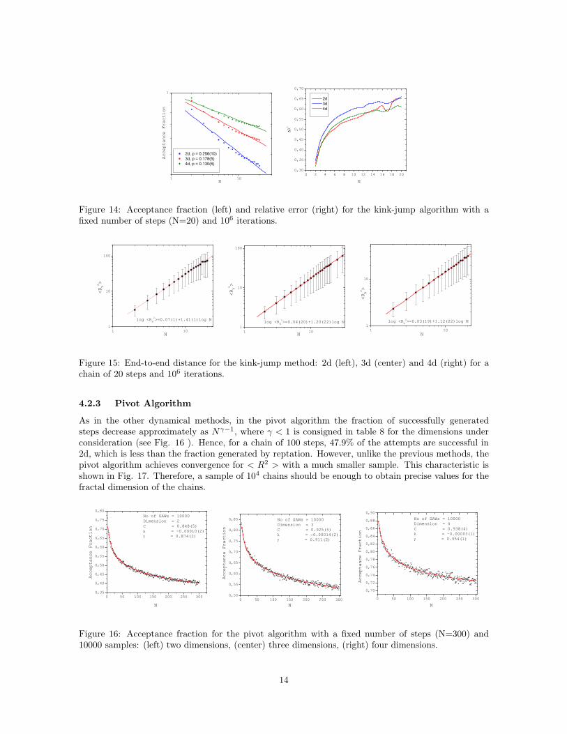
4.2.2 Kink-Jump Algorithm

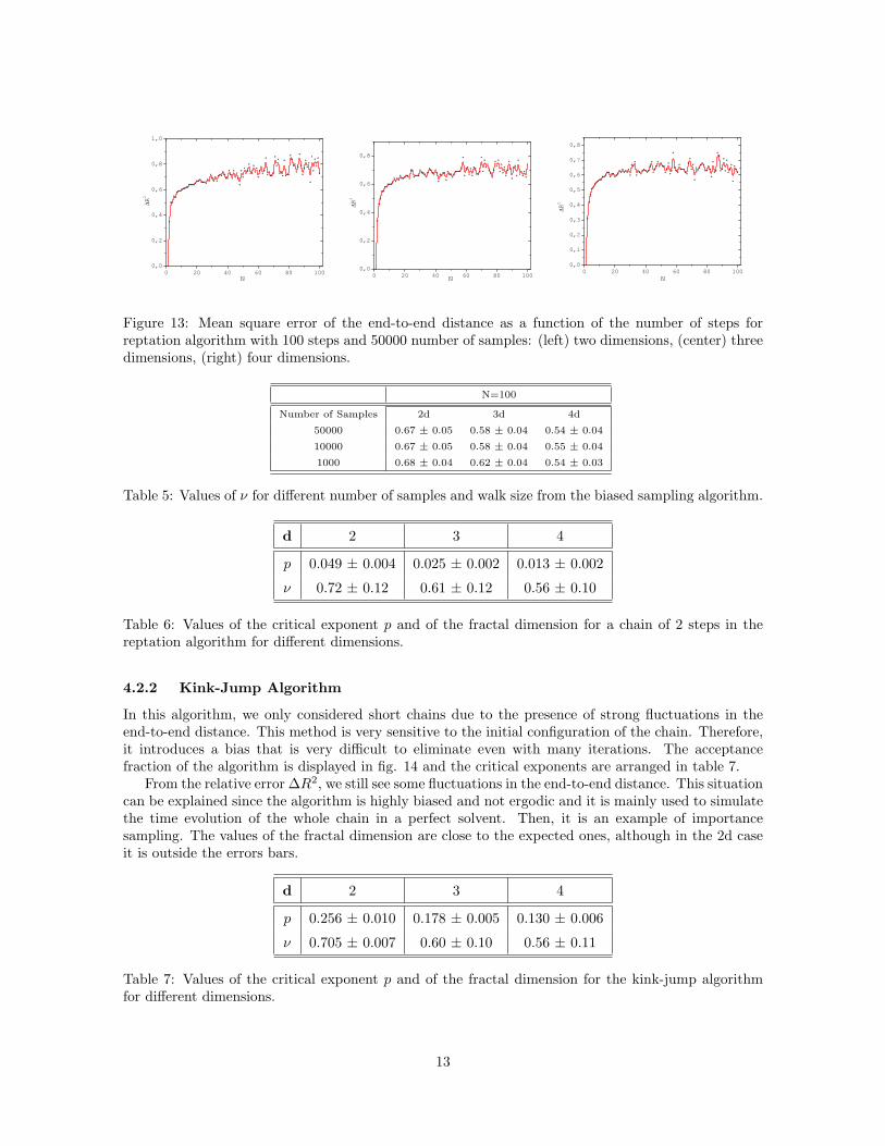
In this algorithm, we only considered short chains due to the presence of strong fluctuations in theend-to-end distance. This method is very sensitive to the initial configuration of the chain. Therefore,it introduces a bias that is very difficult to eliminate even with many iterations. The acceptancefraction of the algorithm is displayed in fig. 14 and the critical exponents are arranged in table 7.

From the relative error ∆R2, we still see some fluctuations in the end-to-end distance. This situationcan be explained since the algorithm is highly biased and not ergodic and it is mainly used to simulatethe time evolution of the whole chain in a perfect solvent. Then, it is an example of importancesampling. The values of the fractal dimension are close to the expected ones, although in the 2d caseit is outside the errors bars.

d 2 3 4

p 0.256 ± 0.010 0.178 ± 0.005 0.130 ± 0.006

ν 0.705 ± 0.007 0.60 ± 0.10 0.56 ± 0.11

Table 7: Values of the critical exponent p and of the fractal dimension for the kink-jump algorithmfor different dimensions.

13

1 10

1

N

Acceptance Fraction

2d, p = 0.256(10) 3d, p = 0.178(5) 4d, p = 0.130(6)

0 2 4 6 8 10 12 14 16 18 20

0,30

0,35

0,40

0,45

0,50

0,55

0,60

0,65

0,70

2d 3d 4d

N

R2

Figure 14: Acceptance fraction (left) and relative error (right) for the kink-jump algorithm with afixed number of steps (N=20) and 106 iterations.

1 101

10

100

log <RN2>=0.07(1)+1.41(1)log N

N

<RN2 >

1 101

10

100

N

<RN2 >

log <RN2>=0.04(20)+1.20(22)log N

1 101

10

N

<RN2 >

log <RN2>=0.03(19)+1.12(22)log N

Figure 15: End-to-end distance for the kink-jump method: 2d (left), 3d (center) and 4d (right) for achain of 20 steps and 106 iterations.

4.2.3 Pivot Algorithm

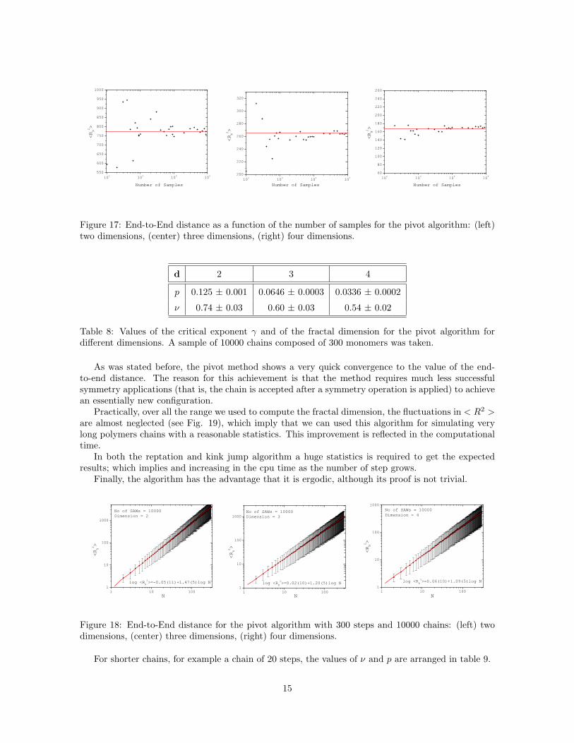
As in the other dynamical methods, in the pivot algorithm the fraction of successfully generatedsteps decrease approximately as Nγ−1, where γ < 1 is consigned in table 8 for the dimensions underconsideration (see Fig. 16 ). Hence, for a chain of 100 steps, 47.9% of the attempts are successful in2d, which is less than the fraction generated by reptation. However, unlike the previous methods, thepivot algorithm achieves convergence for < R2 > with a much smaller sample. This characteristic isshown in Fig. 17. Therefore, a sample of 104 chains should be enough to obtain precise values for thefractal dimension of the chains.

0 50 100 150 200 250 3000,35

0,40

0,45

0,50

0,55

0,60

0,65

0,70

0,75

0,80

N

Acceptance Fraction

No of SAWs = 10000Dimension = 2C = 0.848(5) = -0.00010(2) = 0.874(2)

0 50 100 150 200 250 3000,50

0,55

0,60

0,65

0,70

0,75

0,80

0,85

N

Acceptance Fraction

No of SAWs = 10000Dimension = 3C = 0.925(5) = -0.00014(2) = 0.911(2)

0 50 100 150 200 250 300

0,700,720,740,760,780,800,820,840,860,880,90

N

Acceptance Fraction

No of SAWs = 10000Dimension = 4C = 0.938(4) = -0.00003(1) = 0.954(1)

Figure 16: Acceptance fraction for the pivot algorithm with a fixed number of steps (N=300) and10000 samples: (left) two dimensions, (center) three dimensions, (right) four dimensions.

14

102 103 104 105550

600

650

700

750

800

850

900

950

1000

Number of Samples

<RN2 >

102 103 104 105200

220

240

260

280

300

320

Number of Samples

<RN2 >

102 103 104 1056080100120140160180200220240260

Number of Samples

<RN2 >

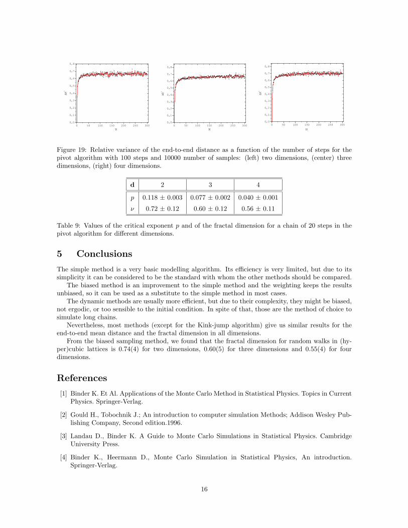
Figure 17: End-to-End distance as a function of the number of samples for the pivot algorithm: (left)two dimensions, (center) three dimensions, (right) four dimensions.

d 2 3 4

p 0.125 ± 0.001 0.0646 ± 0.0003 0.0336 ± 0.0002

ν 0.74 ± 0.03 0.60 ± 0.03 0.54 ± 0.02

Table 8: Values of the critical exponent γ and of the fractal dimension for the pivot algorithm fordifferent dimensions. A sample of 10000 chains composed of 300 monomers was taken.

As was stated before, the pivot method shows a very quick convergence to the value of the end-to-end distance. The reason for this achievement is that the method requires much less successfulsymmetry applications (that is, the chain is accepted after a symmetry operation is applied) to achievean essentially new configuration.

Practically, over all the range we used to compute the fractal dimension, the fluctuations in < R2 >are almost neglected (see Fig. 19), which imply that we can used this algorithm for simulating verylong polymers chains with a reasonable statistics. This improvement is reflected in the computationaltime.

In both the reptation and kink jump algorithm a huge statistics is required to get the expectedresults; which implies and increasing in the cpu time as the number of step grows.

Finally, the algorithm has the advantage that it is ergodic, although its proof is not trivial.

1 10 1001

10

100

1000

log <RN2>=-0.05(11)+1.47(5)log N

<RN2 >

N

No of SAWs = 10000Dimension = 2

1 10 1001

10

100

1000

log <RN2>=0.02(10)+1.20(5)log N

No of SAWs = 10000Dimension = 3

<RN2 >

N

1 10 1001

10

100

1000

<RN2 >

N

log <RN2>=0.06(10)+1.09(5)log N

No of SAWs = 10000Dimension = 4

Figure 18: End-to-End distance for the pivot algorithm with 300 steps and 10000 chains: (left) twodimensions, (center) three dimensions, (right) four dimensions.

For shorter chains, for example a chain of 20 steps, the values of ν and p are arranged in table 9.

15

0 50 100 150 200 250 3000,0

0,1

0,2

0,3

0,4

0,5

0,6

0,7

0,8

N

R2

0 50 100 150 200 250 3000,0

0,1

0,2

0,3

0,4

0,5

0,6

0,7

0,8

N

R2

0 50 100 150 200 250 3000,0

0,1

0,2

0,3

0,4

0,5

0,6

0,7

0,8

N

R2

Figure 19: Relative variance of the end-to-end distance as a function of the number of steps for thepivot algorithm with 100 steps and 10000 number of samples: (left) two dimensions, (center) threedimensions, (right) four dimensions.

d 2 3 4

p 0.118 ± 0.003 0.077 ± 0.002 0.040 ± 0.001

ν 0.72 ± 0.12 0.60 ± 0.12 0.56 ± 0.11

Table 9: Values of the critical exponent p and of the fractal dimension for a chain of 20 steps in thepivot algorithm for different dimensions.

5 Conclusions

The simple method is a very basic modelling algorithm. Its efficiency is very limited, but due to itssimplicity it can be considered to be the standard with whom the other methods should be compared.

The biased method is an improvement to the simple method and the weighting keeps the resultsunbiased, so it can be used as a substitute to the simple method in most cases.

The dynamic methods are usually more efficient, but due to their complexity, they might be biased,not ergodic, or too sensible to the initial condition. In spite of that, those are the method of choice tosimulate long chains.

Nevertheless, most methods (except for the Kink-jump algorithm) give us similar results for theend-to-end mean distance and the fractal dimension in all dimensions.

From the biased sampling method, we found that the fractal dimension for random walks in (hy-per)cubic lattices is 0.74(4) for two dimensions, 0.60(5) for three dimensions and 0.55(4) for fourdimensions.

References

[1] Binder K. Et Al. Applications of the Monte Carlo Method in Statistical Physics. Topics in CurrentPhysics. Springer-Verlag.

[2] Gould H., Tobochnik J.; An introduction to computer simulation Methods; Addison Wesley Pub-lishing Company, Second edition.1996.

[3] Landau D., Binder K. A Guide to Monte Carlo Simulations in Statistical Physics. CambridgeUniversity Press.

[4] Binder K., Heermann D., Monte Carlo Simulation in Statistical Physics, An introduction.Springer-Verlag.

16

[5] Batoulis J., Kremer K.; J.Phys.A: Math. Gen. 21 (1988) 127-146.

[6] Wall, F., Mandel, F.; J. Chem. Phys. 63, 4592 (1975).

[7] Madras, N., Sokal, A.D.; Journal of Statistical Physics Vol. 50, Nos. 1/2, 1988

[8] Haggstrom, Olle. Finite Markov Chains and Algorithmic Applications. Cambridge UniversityPress, 2002.

17