Embed Size (px)
Citation preview

New Method for Composite Optimal Control
of Singularly Perturbed Systems
Hua Xu, Hiroaki Mukaidani and Koichi Mizukami
Faculty of Integrated Arts and Sciences,
Hiroshima University, 1-7-1, Kagamiyama,
Higashi-Hiroshima, Japan 739
Abstract. In this paper, a new method based on a generalized algebraic Riccati equation
arising in descriptor systems is presented to solve the composite optimal control problem of
singularly perturbed systems. Di�erent from the existing method, the slow subsystem is viewed
as a special kind of descriptor systems. A new composite optimal controller is obtained which
is valid for both standard and nonstandard singularly perturbed systems. It is shown that the
composite optimal control can be obtained simply by only revising the solution of the slow
regulator problem. It is proven that the composite optimal control can achieve a performance
which is O("2) close to the optimal performance. Although this result is well-known for the
standard singularly perturbed systems, it is new in the nonstandard case. The equivalence
between the new composite optimal controller and the existing one is also established for the
standard singularly perturbed systems.
Faculty of Integrated Arts and Sciences
Hiroshima University, 1-7-1, Kagamiyama
Higashi-Hiroshima, Japan 739
Email: [email protected]
1
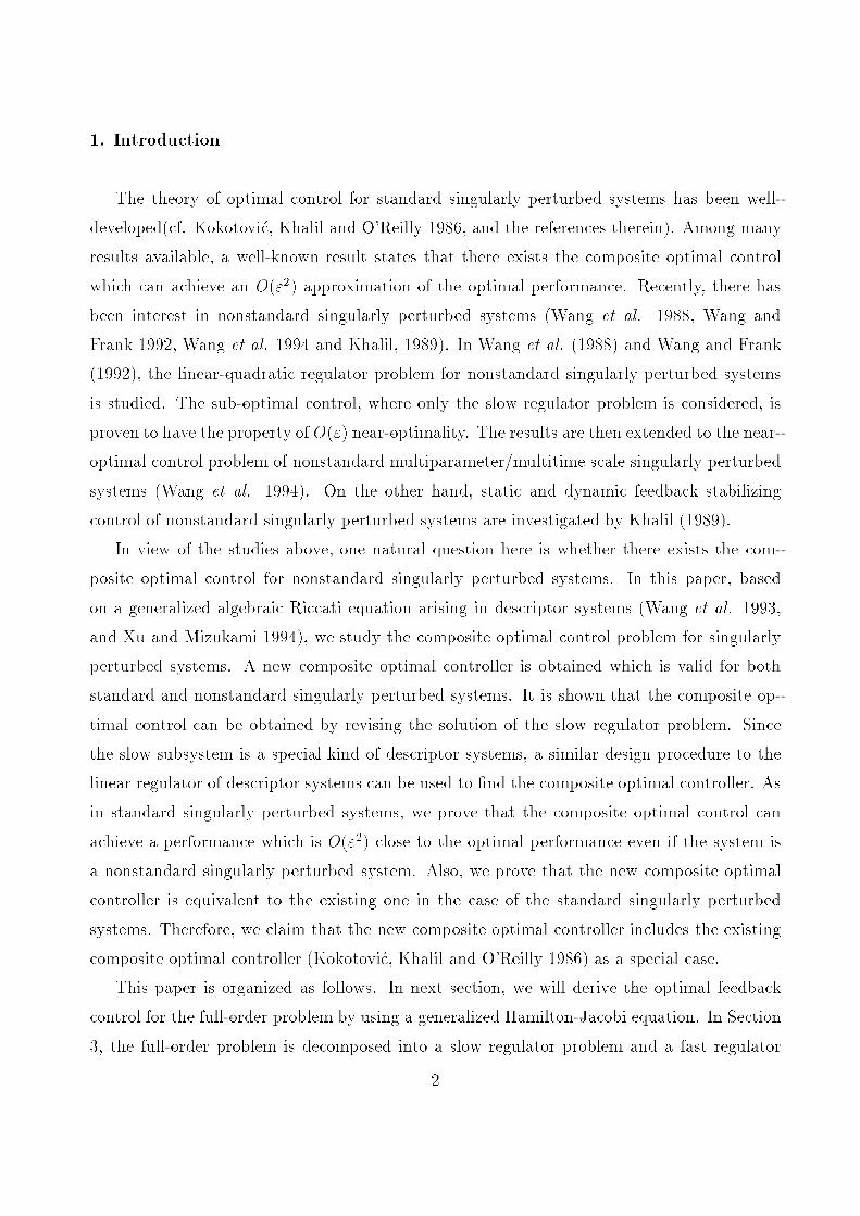
1. Introduction
The theory of optimal control for standard singularly perturbed systems has been well-
developed(cf. Kokotovi�c, Khalil and O'Reilly 1986, and the references therein). Among many
results available, a well-known result states that there exists the composite optimal control
which can achieve an O("2) approximation of the optimal performance. Recently, there has
been interest in nonstandard singularly perturbed systems (Wang et al. 1988, Wang and
Frank 1992, Wang et al. 1994 and Khalil, 1989). In Wang et al. (1988) and Wang and Frank
(1992), the linear-quadratic regulator problem for nonstandard singularly perturbed systems
is studied. The sub-optimal control, where only the slow regulator problem is considered, is
proven to have the property of O(") near-optimality. The results are then extended to the near-
optimal control problem of nonstandard multiparameter/multitime scale singularly perturbed
systems (Wang et al. 1994). On the other hand, static and dynamic feedback stabilizing
control of nonstandard singularly perturbed systems are investigated by Khalil (1989).
In view of the studies above, one natural question here is whether there exists the com-
posite optimal control for nonstandard singularly perturbed systems. In this paper, based
on a generalized algebraic Riccati equation arising in descriptor systems (Wang et al. 1993,
and Xu and Mizukami 1994), we study the composite optimal control problem for singularly
perturbed systems. A new composite optimal controller is obtained which is valid for both
standard and nonstandard singularly perturbed systems. It is shown that the composite op-
timal control can be obtained by revising the solution of the slow regulator problem. Since
the slow subsystem is a special kind of descriptor systems, a similar design procedure to the
linear regulator of descriptor systems can be used to �nd the composite optimal controller. As
in standard singularly perturbed systems, we prove that the composite optimal control can
achieve a performance which is O("2) close to the optimal performance even if the system is
a nonstandard singularly perturbed system. Also, we prove that the new composite optimal
controller is equivalent to the existing one in the case of the standard singularly perturbed
systems. Therefore, we claim that the new composite optimal controller includes the existing
composite optimal controller (Kokotovi�c, Khalil and O'Reilly 1986) as a special case.
This paper is organized as follows. In next section, we will derive the optimal feedback
control for the full-order problem by using a generalized Hamilton-Jacobi equation. In Section
3, the full-order problem is decomposed into a slow regulator problem and a fast regulator
2

problem. Their solutions are investigated. In Section 4, we will construct the new composite
optimal controller and discuss its near-optimality property. The equivalence between the new
composite optimal controller and the existing one is established for the standard singularly
perturbed systems. Section 5 is concerned with the design procedure of the composite optimal
controller. Finally, Section 6 discusses some conclusions.
2. Full-Order Regulator Problem
Consider the linear time-invariant singularly perturbed system
_x = A11x+ A12z +B1u; x(0) = x0; (1a)
" _z = A21x+ A22z +B2u; z(0) = z0; (1b)
with a performance index
J =1
2
Z1
0(
264 x
z
375T
Q
264 x
z
375+ uTRu)dt; (2)
which has to be minimized, where
Q =
264 Q11 Q12
QT12 Q22
375 =
264 CT
1 C1 CT1 C2
CT2 C1 CT
2 C2
375 ; R > 0; (3)
and " is a small positive parameter, x(t) 2 Rn and z(t) 2 Rm are states, and u(t) 2 Rr
is the control, and all matrices are of appropriate dimensions. The system (1) is called the
nonstandard singularly perturbed system if the matrix A22 is singular.
In order to compare the near-optimal performance with the optimal performance in Section
4, we must have an exact expression of the optimal performance. Di�erent from the existing
method (Kokotovi�c et al. 1986 and Chow and Kokotovi�c 1976), we derive the optimal feedback
control for the full-order problem by using a generalized Hamilton-Jacobi equation (Xu and
Mizukami 1993), and arrive at the optimal performance with the new form. Before doing
that, we make a temporary assumption that the �nal time of the performance (2) is �nite and
�xed for the convenience of presentation. Let the optimal performance index for the full-order
problem take the form
V�(E"y(t); t) = (1=2)yT (t)E"P (t)y(t);3
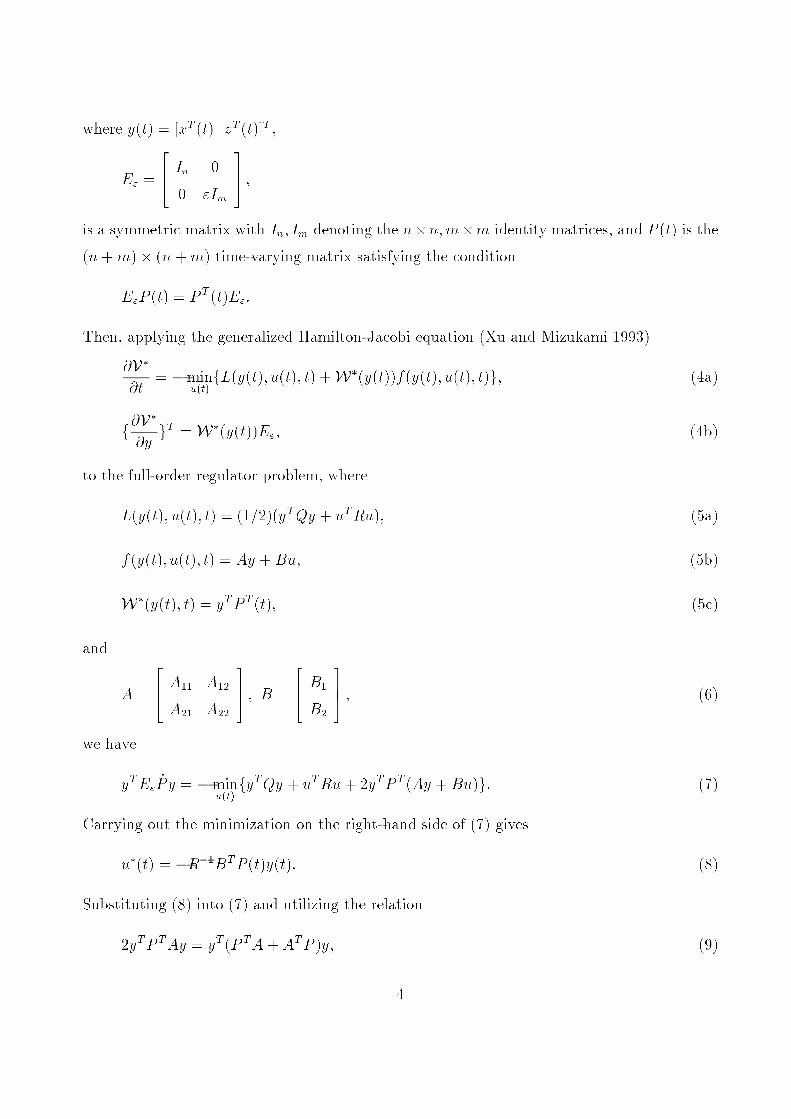
where y(t) = [xT (t) zT (t)]T ,
E" =
264 In 0
0 "Im
375 ;
is a symmetric matrix with In; Im denoting the n�n;m�m identity matrices, and P (t) is the
(n+m)� (n+m) time-varying matrix satisfying the condition
E"P (t) = P T (t)E":
Then, applying the generalized Hamilton-Jacobi equation (Xu and Mizukami 1993)
@V�@t
= �minu(t)fL(y(t); u(t); t) +W�(y(t))f(y(t); u(t); t)g; (4a)
f@V�
@ygT =W�(y(t))E"; (4b)
to the full-order regulator problem, where
L(y(t); u(t); t) = (1=2)(yTQy + uTRu); (5a)
f (y(t); u(t); t) = Ay +Bu; (5b)
W�(y(t); t) = yTP T (t); (5c)
and
A =
264 A11 A12
A21 A22
375 ; B =
264 B1
B2
375 ; (6)
we have
yTE"_Py = �min
u(t)fyTQy + uTRu+ 2yTP T (Ay +Bu)g: (7)
Carrying out the minimization on the right-hand side of (7) gives
u�(t) = �R�1BTP (t)y(t): (8)
Substituting (8) into (7) and utilizing the relation
2yTP TAy = yT (P TA+ ATP )y; (9)
4
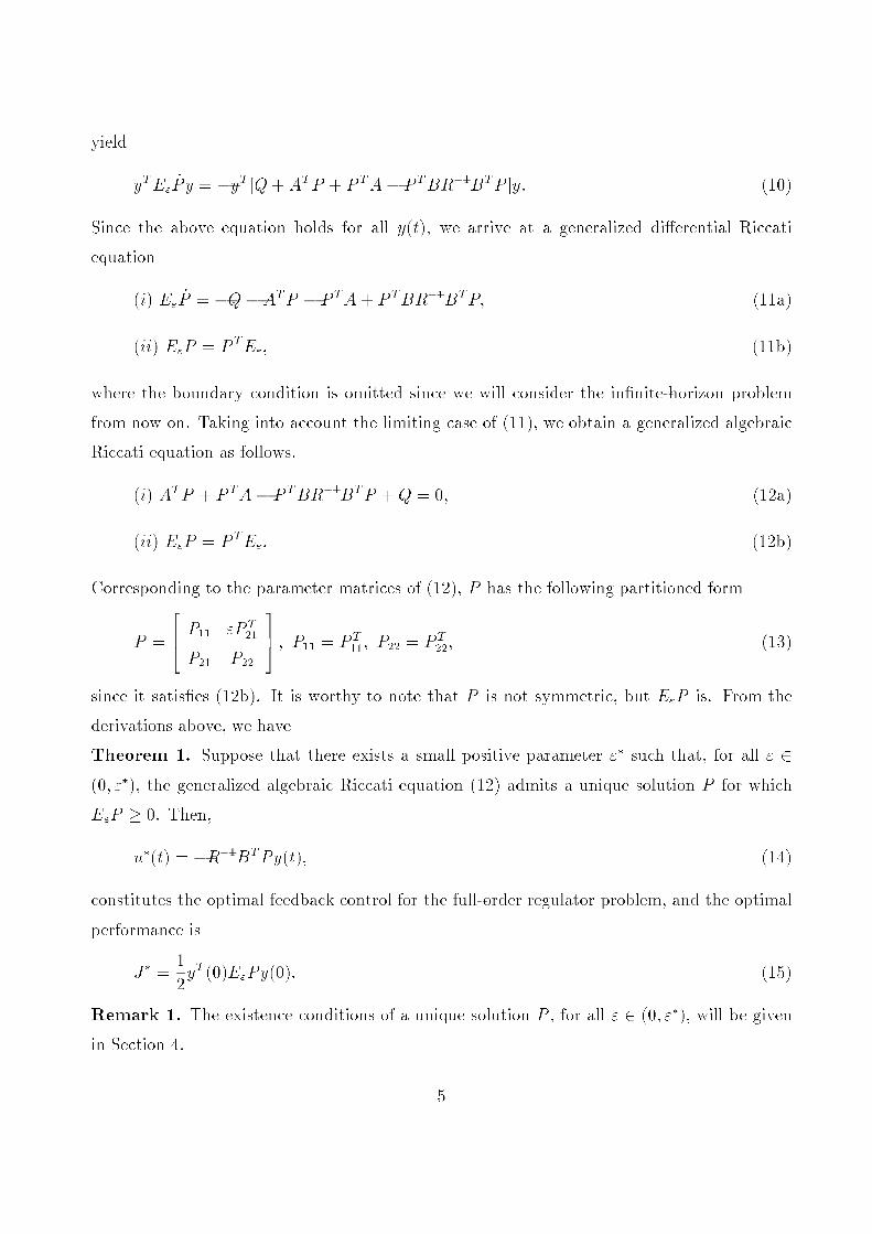
yield
yTE"_Py = �yT [Q+ ATP + P TA� P TBR�1BTP ]y: (10)
Since the above equation holds for all y(t), we arrive at a generalized di�erential Riccati
equation
(i) E"_P = �Q� ATP � P TA+ P TBR�1BTP; (11a)
(ii) E"P = P TE"; (11b)
where the boundary condition is omitted since we will consider the in�nite-horizon problem
from now on. Taking into account the limiting case of (11), we obtain a generalized algebraic
Riccati equation as follows.
(i) ATP + P TA� P TBR�1BTP +Q = 0; (12a)
(ii) E"P = P TE": (12b)
Corresponding to the parameter matrices of (12), P has the following partitioned form
P =
264 P11 "P T
21
P21 P22
375 ; P11 = P T
11; P22 = P T22; (13)
since it satis�es (12b). It is worthy to note that P is not symmetric, but E"P is. From the
derivations above, we have
Theorem 1. Suppose that there exists a small positive parameter "� such that, for all " 2(0; "�), the generalized algebraic Riccati equation (12) admits a unique solution P for which
E"P � 0. Then,
u�(t) = �R�1BTPy(t); (14)
constitutes the optimal feedback control for the full-order regulator problem, and the optimal
performance is
J� =1
2yT (0)E"Py(0): (15)
Remark 1. The existence conditions of a unique solution P , for all " 2 (0; "�), will be given
in Section 4.
5

3. Decomposition of Slow and Fast Regulator Problems
Similar to the standard singularly perturbed systems, we decompose the full-order regulator
problem into two subsystem regulator problems.
Slow regulator problem: Find us to minimize
Js =1
2
Z1
0(
264 xs
zs
375T
Q
264 xs
zs
375+ uTs Rus)dt; (16)
for the slow subsystem
E _ys = Ays +Bus; Eys(0) = Ey0; (17)
where ys(t) = [xTs (t) zTs (t)]T , E = E"j"=0, A, B are de�ned in (6), and Q in (3).
Remark 2. The slow subsystem (17) is formed by neglecting the fast mode, which is equivalent
to letting " = 0 in (1). Di�erent from the existing method to decompose the full-order system
into the slow and fast subsystems, we do not use the inverse of A22, which does not exist
in a nonstandard case, to eliminate zs in (16),(17). The slow subsystem (17) is viewed as a
descriptor system which may display an impulse phenomenon in the solution if A22 is singular.
It is clear that the descriptor system method permits us to study the standard and nonstandard
singularly perturbed system in a uni�ed way.
Fast regulator problem: Find uf to minimize
Jf =1
2
Z1
0(zTf C
T2 C2zf + uTfRuf )dt; (18)
for the fast subsystem
" _zf = A22zf +B2uf ; zf(0) = z0 � zs(0); (19)
where zf = z � zs, uf = u� us.
The fast subsystem (19) is derived by assuming that the slow variables are constant during
fast transients, that is, _zs = 0 and xs = a constant.
We now consider the solution of the slow and fast regulator problems under the following
assumptions.
Assumption 1. The slow subsystem (17) is stabilizable and detectable, that is, for all s with
Re[s] � 0,
Rank
264 sIn � A11 �A12 B1
�A21 �A22 B2
375 = n+m; (20a)
6

Rank
264 sIn � AT
11 �AT21 CT
1
�AT12 �AT
22 CT2
375 = n +m: (20b)
Assumption 2. The fast subsystem (19) is stabilizable and detectable.
Let us �rst consider the solution of the fast regulator problem.
Proposition 1. Under Assumption 2, the fast regulator problem admits a unique optimal
feedback control
u�f = �R�1B22P+22fzf ; (21)
where P+22f is a unique stabilizing positive semide�nite symmetric solution of the algebraic
Riccati equation
P22fA22 + AT22P22f � P22fB2R
�1BT2 P22f + Q22 = 0: (22)
The slow regulator problem is similar to the regulator problem of descriptor systems except
that di�erent assumptions on the system parameters are required in two problems. In other
words, for the existence of the fast regulator problem, Assumption 2 is reasonable in the study
of the slow regulator problem. However, this assumption is unnecessarily strong in the study
of the regulator problem for a general descriptor system. Instead of Assumption 2, we only
need to assume that the system (17) is impulsively controllable and observable if it is a general
descriptor system, that is,
Rank[A22 B2] = m; Rank[AT22 CT
2 ] = m: (23)
Obviously, Assumption 2 implies the conditions (23), but not vice versa.
In the following, we will consider the solution of the slow regulator problem. Before doing
that, we �rst introduce another generalized algebraic Riccati equation (Wang et al. 1993, and
Xu and Mizukami 1994),
(i) ATPs + P Ts A� P T
s BR�1BTPs +Q = 0; (24a)
(ii) ETPs = P Ts E: (24b)
where Q is the same as that in (12). The solution Ps of (24) has a lower-triangular block form
Ps =
264 P11s 0
P21s P22s
375 ; PT
11s = P11s; (25)
7

because of (24b). It is worthy to note that P22s may not be symmetric. The algebraic Riccati
equation (24) can be partitioned into
P11sA11 + P T21sA21 + AT
11P11s + AT21P21s � P11sS11P11s
�P T21sS
T12P11s � P11sS12P21s � P T
21sS22P21s +Q11 = 0; (26a)
P T22sA21 + AT
12P11s + AT22P21s � P T
22sST12P11s � P T
22sS22P21s +QT12 = 0; (26b)
P T22sA22 + AT
22P22s � P T22sS22P22s +Q22 = 0; (26c)
where
S11 = B1R�1BT
1 ; S12 = B1R�1BT
2 ; S22 = B2R�1BT
2 : (27)
The equation (26c) is an algebraic Riccati equation which admits at least a stabilizing positive
semide�nite symmetric solution under Assumption 2. Moreover, Assumption 2 ensures that
A22 � S22P22s is nonsingular (see proof of Lemma 1 below). Substituting the solution of (26c)
into (26b) yields
P21s = �NT2s +NT
1sP11s; (28)
where
NT2s = A�T22sQ
T12s; NT
1s = �A�T22sAT12s;
A12s = A12 � S12P22s; A22s = A22 � S22P22s;
Q12s = Q12 + AT21P22s:
Furthermore, substituting P21s into (26a) and making some lengthy calculations (the detail is
omitted for brevity), we get
P11sAs + ATs P11s � P11sSsP11s +Qs = 0; (29)
where
Qs = Q11 �N2sA21 � AT21N
T2s �N2sS22N
T2s; (30a)
As = A11 +N1sA21 + S12NT2s +N1sS22N
T2s; (30b)8

Ss = S11 +N1sST12 + S12N
T1s +N1sS22N
T1s: (30c)
Lemma 1. Under Assumptions 1,2, the following results hold.
(i) The algebraic Riccati equations (29) is decoupled to the algebraic Riccati equation
(26c).
(ii) There exist a n�r matrix Bs and a matrix Cs with the same dimension as C1 such that
Ss = BsR�1BT
s , Qs = CTs Cs. Moreover, the triple (As; Bs; Cs) is stabilizable and detectable.
Proof. see Appendix A. ■
Since the triple (As; Bs; Cs) is stabilizable and detectable, the algebraic Riccati equation
(29) admits a unique stabilizing positive semide�nite symmetric solution, denoted by P+11s, and
As � SsP+11s is Hurwitz.
Proposition 2. Under Assumptions 1, 2, the slow regulator problem admits a unique optimal
open-loop control, which can be implemented by a class of linear feedback controls given by
u�s = �R�1BTPsys; (31)
where
Ps =
264 P+
11s 0
P21s P22s
375 ; (32)
is the solution of the generalized algebraic Riccati equation (24).
Proof. First, we prove that the linear feedback controls (31) are strictly feedback stabilizing
and under which xs(t); zs(t) are impulse-free and xs(t) ! 0, zs(t) ! 0 as t ! 1 for all Ey0.
Substituting (31) into (17) yields264 In 0
0 0
375264 _xs
_zs
375 =
264 A11s A12s
A21s A22s
375264 xs
zs
375 ; (33)
where A12s, A22s are de�ned under the equation (28), and
A11s = A11 � S11P+11s � S12P21s; A21s = A21 � S21P
+11s � S22P21s:
Since A22s is nonsingular from the proof of Lemma 1, (33) can be further transformed to a
standard state space system and an algebraic equation
_xs = (A11s � A12sA�122sA21s)xs; (34a)
zs = �A�122sA21sxs: (34b)9
Moreover, xs(t), zs(t) are impulse free for the same reason. Now, if we can prove that the
system matrix of (34a) is As � SsP+11s, then we have xs(t) ! 0, as t ! 1. That also implies
zs(t) ! 0 as t ! 1. Substituting (28) into the system matrix of (34a) and making some
manipulations yield
A11s � A12sA�122sA21s = A11 � S11P
+11s � S12(N
T1sP
+11s �NT
2s)
+N1s[A21 � S21P+11s � S22(N
T1sP
+11s �NT
2s)]
= A11 +N1sA21 + S12NT2s +N1sS22N
T2s � (S11 +N1sS
T12 + S12N
T1s +N1sS22N
T1s)P
+11s
= As � SsP+11s: (35)
Therefore, (31) are the strictly feedback stabilizing controls.
Secondly, from the derivations before the proposition, we have known that Ps is a solution
of the generalized algebraic Riccati equation (24).
Finally, we will prove that (31) is really a optimal feedback control by using a \completion
of squares" method. Utilizing the algebraic Riccati equation (24) in (16), (17), we have
1
2yTs (T )E
TPsys(T ) � 1
2yT0 E
TPsy0 =1
2
Z T
0
d
dt[yTs E
TPsys]dt
=1
2
Z T
0yTs [�ATPs � P T
s A+ P Ts BR
�1BTPs �Q]ysdt
+1
2
Z T
0[ _yTs E
TPsys + yTs PTs E _ys]dt; (36)
Substituting E _ys(t) into (36) yields
1
2yTs (T )E
TPsys(T ) � 1
2yT0 E
TPsy0
=1
2
Z T
0[uTs B
TPsys + yTs PTs Bus � yTs Qys + yTs P
Ts BR
�1BTPsys]dt: (37)
Moving the left side of (37) to the right and adding Js(us;T ) to the both sides of it give
Js(us;T ) =1
2yT0 E
TPsy0 � 1
2yTs (T )E
TPsys(T )
+1
2
Z T
0f[us +R�1BTPsys]
TR[us +R�1BTPsys]gdt: (38)
10
Letting T !1 and noting ys(t)! 0 as t!1 for all admissible us, we have
Js(us;1) =1
2yT0 E
TPsy0 +1
2
Z1
0f[us +R�1BTPsys]
TR[us +R�1BTPsys]gdt: (39)
Since the �rst term above is independent of us and ETPs is unique (since P+11s is unique), it is
obvious that u�s given by (31) is the optimal feedback control. ■
Remark 2. The results of Proposition 2 can also be deduced from the corresponding results
of the regulator problem of descriptor systems (Wang et al. 1993 and Xu and Mizukami 1994).
However, the proof there is not so complete. Here, we have provided a di�erent, complete and
self-contained proof.
Remark 3. Similar to descriptor systems, an important feature of the slow regulator problem
is that the optimal feedback controls are not unique. This fact is easily seen by noting that any
solution of the algebraic Riccati equation (26c) can be used in the feedback gain of (31). But
ETPs = P Ts E � 0 is unique since only P+
11s � 0, the unique stabilizing positive semide�nite
symmetric solution of (29), is allowed in the feedback gain of (31).
4. Near-Optimality of Composite Optimal Control
In this section, we will construct the composite optimal control u�c = u�s+u�f as in standard
case (Kokotovi�c et al. 1986). It has been known that the optimal feedback control for the slow
regulator problem is not unique. However, the corresponding optimal feedback control for the
fast regulator problem is unique. We will select a particular optimal feedback control of the
slow regulator problem to construct the composite optimal control, that is,
u�+s = �R�1BTP+s ys; (40)
where
P+s =
264 P+
11s 0
P+21s P+
22s
375 ; (41)
P+22s is the unique stabilizing positive semide�nite symmetric solution of the algebraic Riccati
equation (26c), and P+21s is the corresponding one in (28) with P22s = P+
22s, P11s = P+11s.
Now, comparing (26c) with (22), we readily have an important relation P+22s = P+
22f . As
the result, we obtain
u�c = u�+s + u�f = �R�1[BT1 BT
2 ]
264 P+
11s 0
P+21s P+
22s
375264 xs
zs
375�R�1BT
2 P+22fzf
11

= �R�1[BT1 BT
2 ]
264 P+
11s 0
P+21s P+
22s
375264 x
z
375 ; (42)
where x(t) � xs(t) and z(t) � zs(t) + zf (t).
Remark 4. Let us compare (42) with (40). Then, we can �nd that u�+s is di�erent from u�c
only in P22s, P21s and ys. This fact implies that u�c(t) can be obtained very simply by solving
the slow regulator problem (the design procedure will be given in Section 5), and then revising
its solution. In other words, we can select P+22s as the solution of (26c), and change the slow
variable ys to the original variable y in (40) to obtain the composite optimal control u�c .
We now apply the composite optimal control u�c to the full-order system (1) and compare it
with the exact optimal control (14). In order to do that, we �rst study the existence conditions
of the unique solution P of the generalized algebraic Riccati equation (12).
Theorem 2. Under Assumptions 1, 2, there exists a small positive parameter "� such that,
for all " 2 [0; "�), the generalized algebraic Riccati equation (12) admits a unique stabilizing
solution P for which E"P � 0. Moreover, the solution P possesses a power series expansion
at " = 0, that is,
P =
264 P
(0)11 "P
(0)T21
P(0)21 P
(0)22
375+
1Xi=1
"i
i!
264 P
(i)11 "P
(i)T21
P(i)21 P
(i)22
375 : (43)
Proof. The algebraic Riccati equation (12) can be partitioned into
AT11P11 + P11A11 + AT
21P21 + P T21A21 � P11S11P11
�P T21S22P21 � P11S12P21 � P T
21ST12P11 +Q11 = 0; (44a)
"P21A11 + P22A21 + AT12P11 + AT
22P21 � "P21S11P11
�"P21ST12P21 � P22S
T12P11 � P22S22P21 +QT
12 = 0; (44b)
AT22P22 + P22A22 + "AT
12PT21 + "P21A12 � P22S22P22
�"P22ST12P
T21 � "P21S12P22 � "2P21S
T11P
T21 +Q22 = 0: (44c)
Let " = 0, then the zero-order equations in (44) reduce to
P(0)11 A11 + P
(0)T21 A21 + AT
11P(0)11 + AT
21P(0)21 � P
(0)11 S11P
(0)11
12

�P (0)T21 ST
12P(0)11 � P
(0)11 S12P
(0)21 � P
(0)T21 S22P
(0)21 +Q11 = 0; (45a)
P(0)22 A21 + AT
12P(0)11 + AT
22P(0)21 � P
(0)22 S
T12P
(0)11 � P
(0)22 S22P
(0)21 + QT
12 = 0; (45b)
P(0)22 A22 + AT
22P(0)22 � P
(0)22 S22P
(0)22 +Q22 = 0: (45c)
The zero-order equations in (45) are the same as those in (26) except that P (0)22 here is required
to be symmetric. Hence, (45) has a solution P(0)11 = P+
11s, P(0)22 = P+
22s and P(0)21 = P+
21s
under Assumptions 1 and 2. Furthermore, applying the implicit function theorem at the point
(" = 0; P11 = P(0)11 ; P21 = P
(0)21 ; P22 = P
(0)22 ) to the equations (44) yields the following Jacobian
matrix.
Jacobi =
266664J11 J12 J13
J21 J22 J23
J31 J32 J33
377775(0;P
(0)11 ;P
(0)21 ;P
(0)22 ):
(46)
Using the Kronecker product representation, we have
J31 = 0; J32 = 0; J33 = Im (A22 � S22P(0)22 ) + (A22 � S22P
(0)22 )
T Im; (47)
from (44c), and
J22 = (A22 � S22P(0)22 )
T In; (48)
from (44b). Furthermore, from (44b), we have
P21 = �NT2 +NT
1 P11 +O("); (49)
where
NT2 = A�T22 Q
T12; NT
1 = �A�T22 AT12;
A12 = A12 � S12P22; A22 = A22 � S22P22;
Q12 = Q12 + AT21P22:
Substituting (49) into (44a) and calculating its derivative with respect to P11 at the point
(" = 0; P11 = P(0)11 ; P21 = P
(0)21 ; P22 = P
(0)22 ) yield
J11 = In [A11 +N1sA21 + S12NT2s +N1sS22N
T2s
13
�(S11 +N1sST12 + S12N
T1s +N1sS22N
T1s)P
+11s]
+[A11 +N1sA21 + S12NT2s +N1sS22N
T2s
�(S11 +N1sST12 + S12N
T1s +N1sS22N
T1s)P
+11s]
T In
= In (As � SsP+11s) + (As � SsP
+11s)
T In; (50)
by noting P(0)11 = P+
11s, P(0)22 = P+
22s and P(0)21 = P+
21s. The exact expressions of J13, J21 and
J23 are not important in the analysis of the nonsingularity of Jacobian matrix Jacobi. Since
(A22 � S22P+22s) and (As � SsP
+11s) are all Hurwitz matrices, J11, J22 and J33 are nonsingular.
Therefore,
Jacobi =
266664J11 0 J13
J21 J22 J23
0 0 J33
377775 ; (51)
is nonsingular. Consequently, there exists a small positive parameter "� such that, for all
" 2 [0; "�), the generalized algebraic Riccati equation (12) admits a unique stabilizing solution
P for which E"P � 0. The property E"P � 0 follows from Q � 0 and R > 0. The uniqueness
of E"P � 0 follows from the fact that P (0)11 = P+
11s and P(0)22 = P+
22s, hence P(0)21 = P+
21s, are all
unique. Finally, the existence of the series (43) at " = 0 follows also from the implicit function
theorem (Dieudonn�e 1982). ■
Remark 5. Similar to the standard case (Kokotovi�c et al. 1986), the existence conditions for
the solution of the full-order regulator problem are also described in terms of stabilizability-
detectability conditions on the slow and fast regulator problems, which are "-independent
(Assumptions 1 and 2). Moreover, it has been proven that Assumption 1 is equivalent to the
assumption that (As; Bs; Cs) is stabilizable and detectable (Lemma 1), a lower-order system
condition.
Now, we can compare the composite optimal control u�c with the exact optimal control u�
and show the O("2) approximation of J�. Applying the composite optimal control u�c to the
full-order system (1), we have
J c =1
2yT (0)E"Pcy(0); (52)
where Pc is the solution of the generalized Lyapunov equation
(i) (A� SP+s )
TPc + P Tc (A� SP+
s ) = �P+Ts SP+
s �Q; (53a)14
(ii) E"Pc = P Tc E"; (53b)
with S = BR�1BT .
Theorem 3. Under the conditions of Theorem 2, the �rst two terms of the power series of J c
and J� at " = 0 are the same, that is,
J c = J� +O("2); (54)
and hence the composite optimal control (42) is an O("2) near-optimal solution to the full-order
regulator problem (1),(2).
Proof. Subtracting (12) from (53) and rearranging, we obtain a generalized Lyapunov equa-
tion for W = Pc � P :
(i) (A� SP+s )
TW +WT (A� SP+s ) = �(P � P+
s )TS(P � P+
s ); (55a)
(ii) E"W = W TE": (55b)
Also from the application of the implicit function theorem to (53), Pc possesses a power series
at " = 0. Thus W can also be extended as follows:
W =
264 W
(0)11 "W
(0)T21
W(0)21 W
(0)22
375+
1Xi=1
"i
i!
264 W
(i)11 "W
(i)T21
W(i)21 W
(i)22
375 : (56)
From (41), (42) and the result that P (0)11 = P+
11s and P(0)22 = P+
22s, we have
(P � P+s )
TS(P � P+s ) = O("2); (57)
and, since (A22 � S22P+22s) and (As � SsP
+11) are Hurwitz matrices, the substitution of (56)
into (55) yields W (0)11 = 0, W (0)
21 = 0, W (0)22 = 0, and W
(1)11 = 0, W (1)
21 = 0, W (1)22 = 0. Hence,
E"W = O("2); which proves (54). ■
We have therefore provided a complete theoretic analysis of the near-optimality of the
composite optimal control for both standard and nonstandard singularly perturbed systems.
To the end of this section, we will show that the composite optimal controller (42) is equivalent
to the existing composite optimal controller (Kokotovi�c et al. 1986) in the case of the standard
singularly perturbed systems. Let A22 of (1) be nonsingular, that is, the standard singularly
perturbed system. Then, the composite optimal controller is
u�c = �R�1�BT1 BT
2 ="
� 264 Ks 0
"KTm "Kf
375264 x
z
375
15

= �R�1�BT1 BT
2
� 264 Ks 0
KTm Kf
375264 x
z
375 : (58)
In the above, Ks is the unique stabilizing positive semide�nite symmetric solution of the
algebraic Riccati equation
0 = �Ks(A0 �B0R�10 NT
0 M0)� (A0 � B0R�10 NT
0 M0)TKs
+KsB0R�10 BT
0 Ks �MT0 (I �N0R
�10 NT
0 )M0; (59)
where
R0 = R+NT0 N0; (60a)
A0 = A11 � A12A�122 A21; B0 = �A12A
�122 B2 +B1; (60b)
M0 = C1 � C2A�122 A21; N0 = �C2A
�122 B2; (60c)
Kf is the unique stabilizing positive semide�nite solution of the algebraic Riccati equation
0 = �KfA22 � AT22Kf +KfB2R
�1BT2 Kf � CT
2 C2; (61)
and Km is
Km = [Ks(B1R�1BT
2 Kf � A12)� (AT21Kf + CT
1 C2)](A22 �B2R�1BT
2 Kf)�1: (62)
Theorem 4. Suppose that the system (1) is the standard singularly perturbed system and
Assumptions 1, 2 are satis�ed. Then, the following identities hold.
Kf = P+22s; KT
m = P+21s; Ks = P+
11s; (63)
and hence the composite optimal controller (58) is the same as the composite optimal controller
(42).
Proof. see Appendix B. ■
From Theorem 4, we claim that the new composite optimal controller includes the existing
composite optimal controller (Kokotovi�c, Khalil and O'Reilly 1986) as the special case.
5. Design Procedure and Example
16
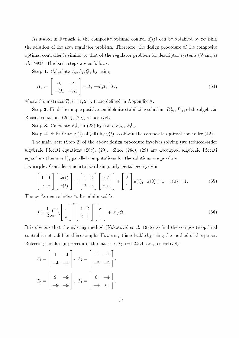
As stated in Remark 4, the composite optimal control u�c(t) can be obtained by revising
the solution of the slow regulator problem. Therefore, the design procedure of the composite
optimal controller is similar to that of the regulator problem for descriptor systems (Wang et
al. 1993). The basic steps are as follows.
Step 1. Calculate As; Ss; Qs by using
Hs :=
264 As �Ss
�Qs �As
375 = T1 � T2T
�14 T3; (64)
where the matrices Ti; i = 1; 2; 3; 4; are de�ned in Appendix A.
Step 2. Find the unique positive semide�nite stabilizing solutions P+22s, P
+11s of the algebraic
Riccati equations (26c), (29), respectively.
Step 3. Calculate P+21s in (28) by using P+
22s, P+11s.
Step 4. Substitute ys(t) of (40) by y(t) to obtain the composite optimal controller (42).
The main part (Step 2) of the above design procedure involves solving two reduced-order
algebraic Riccati equations (26c), (29). Since (26c), (29) are decoupled algebraic Riccati
equations (Lemma 1), parallel computations for the solutions are possible.
Example. Consider a nonstandard singularly perturbed system264 1 0
0 "
375264 _x(t)
_z(t)
375 =
264 1 2
2 0
375264 x(t)
z(t)
375+
264 2
1
375u(t); x(0) = 1; z(0) = 1: (65)
The performance index to be minimized is
J =1
2
Z1
0f264 x
z
375T 264 4 2
2 1
375264 x
z
375+ u2gdt: (66)
It is obvious that the existing method (Kokotovi�c et al. 1986) to �nd the composite optimal
control is not valid for this example. However, it is solvable by using the method of this paper.
Referring the design procedure, the matrices Ti, i=1,2,3,4, are, respectively,
T1 =
264 1 �4�4 �1
375 ; T2 =
264 2 �2�2 �2
375 ;
T3 =
264 2 �2�2 �2
375 ; T4 =
264 0 �1�1 0
375 :
17
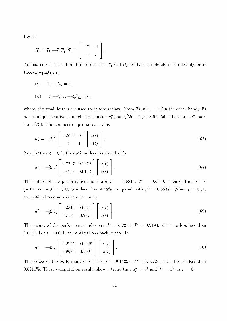
Hence
Hs = T1 � T2T�14 T3 =
264 �7 �4�4 7
375 :
Associated with the Hamiltonian matrices T4 and Hs are two completely decoupled algebraic
Riccati equations,
(i) 1 � p222s = 0;
(ii) 2 � 7p11s � 2p211s = 0;
where, the small letters are used to denote scalars. From (i), p+22s = 1. On the other hand, (ii)
has a unique positive semide�nite solution p+11s = (p65 � 7)=4 � 0:2656. Therefore, p+21s = 4
from (28). The composite optimal control is
u�c = �[2 1]
264 0:2656 0
4 1
375264 x(t)
z(t)
375 : (67)
Now, letting " = 0:1, the optimal feedback control is
u� = �[2 1]
264 0:7217 0:2472
2:4723 0:9158
375264 x(t)
z(t)
375 : (68)
The values of the performance index are J c = 0:6845, J� = 0:6539. Hence, the loss of
performance Jc = 0:6845 is less than 4:48% compared with J� = 0:6539. When " = 0:01,
the optimal feedback control becomes
u� = �[2 1]
264 0:3544 0:0371
3:714 0:997
375264 x(t)
z(t)
375 : (69)
The values of the performance index are J c = 0:2216, J� = 0:2193, with the loss less than
1:08%. For " = 0:001, the optimal feedback control is
u� = �[2 1]
264 0:2755 0:00397
3:9676 0:9997
375264 x(t)
z(t)
375 : (70)
The values of the performance index are J c = 0:14227, J� = 0:14224, with the loss less than
0:0211%. These computation results show a trend that u�c ! u� and Jc ! J� as "! 0.
18
6. Conclusions
In this paper, using the generalized algebraic Riccati equation arising in descriptor systems,
we have studied the composite optimal regulator problem for singularly perturbed systems.
The new composite optimal controller has been obtained which is valid for both standard and
nonstandard singularly perturbed systems. We show that the composite optimal control can
be obtained simply by a procedure of solving the slow regulator problem, and then revising its
solution. Moreover, the existence conditions for the solution of the full-order regulator problem
can also be described in terms of the stabilizability-detectability conditions of the slow and
fast regulator problems which are "-independent and lower-order. As in standard singularly
perturbed systems, we prove that the composite optimal control can achieve a performance
which is O("2) close to the optimal performance even if the system is a nonstandard singularly
perturbed system. Finally, we prove that the new composite optimal controller is equivalent to
the existing one in the case of the standard singularly perturbed systems. Therefore, we claim
that the new composite optimal controller includes the existing composite optimal controller
(Kokotovi�c, Khalil and O'Reilly 1986) as a special case.
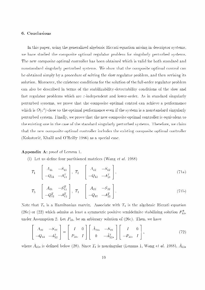
Appendix A: proof of Lemma 1.
(i) Let us de�ne four partitioned matrices (Wang et al. 1988)
T1 =
264 A11 �S11�Q11 �AT
11
375 ; T2 =
264 A12 �S12�Q12 �AT
21
375 ; (71a)
T3 =
264 A21 �ST
12
�QT12 �AT
12
375 ; T4 =
264 A22 �S22�Q22 �AT
22
375 : (71b)
Note that T4 is a Hamiltonian matrix. Associate with T4 is the algebraic Riccati equation
(26c) or (22) which admits at least a symmetric positive semide�nite stabilizing solution P+22s
under Assumption 2. Let P22s be an arbitrary solution of (26c). Then, we have264 A22 �S22�Q22 �AT
22
375 =
264 I 0
P22s I
375264 A22s �S22
0 �AT22s
375264 I 0
�P22s I
375 ; (72)
where A22s is de�ned below (28). Since T4 is nonsingular (Lemma 1, Wang et al. 1988), A22s
19

is also nonsingular. This means that T�14 can be expressed explicitly in terms of A�122s. Fur-
thermore, the algebraic Riccati equation (29) corresponds to the Hamiltonian matrix, namely,
Hs :=
264 As �Ss
�Qs �ATs
375 : (73)
Therefore, it su�ces the proof of (i) to show that Hs = T1 � T2T�14 T3. This can be done by a
lengthy, but direct algebraic manipulations, which are omitted here for brevity.
(ii) From (30c), it is seen that Bs = B1 + N1sB2. However, it seems di�cult to �nd Cs
from (30a). In order to do that, we introduce a dual algebraic Riccati equation of (26c), that
is,
A22K22s +K22sAT22 �K22sQ22K22s + S22 = 0; (74)
which admits at least a symmetric positive semide�nite solution K+22s under Assumption 2.
Similar to the analysis of (72), we have264 A22 �S22�Q22 �AT
22
375 =
264 I �K22s
0 I
375264
~A22s 0
�Q22 � ~AT22s
375264 I K22s
0 I
375 ; (75)
where ~A22s = AT22 � Q22K22s is nonsingular since T4 is nonsingular. After the calculation of
T1 � T2T�14 T3, we arrive at another set of expressions for As, Ss and Qs, that is,
Qs = Q11 +Q12MT2s +M2sQ
T12 +M2sQ22M
T2s; (76a)
As = A11 +M1sQT12 + A12M
T2s +M1sQ22M
T2s; (76b)
Ss = S11 � A12MT1s �M1sA
T12 �M1sQ22M
T1s; (76c)
M1s = ~S12s ~A�122s; M2s = � ~A21s
~A�122s; (76d)
~A21s = AT21 �Q12W22s; ~S12s = S12 + AT
12W22s: (76e)
Hence, it is easy to �nd Cs = C1 + C2MT2s from (76a).
Let us now prove the second part of (ii). Note the relation264 In �A12sA
�122s
0 �A�122s
375264 sIn � A11 �A12 B1
�A21 �A22 B2
375
20

�
266664
In 0 0
�A�122sA21 Im A�122sB2
�BT2 P22sA
�122sA21 BT
2 P22s Ir +BT2 P22sA
�122sB2
377775
=
264 sIn � (A11 + N1sA21) 0 Bs
0 Im 0
375 ; (77)
where the formulas under the equation (28) have been used in the above to simplify the
expressions. Hence,
rank
264 sIn � A11 �A12 B1
�A21 �A22 B2
375 = n+m; for all s with Re[s] � 0; (78)
if and only if rank[sIn� (A11+N1sA21) Bs] = n; for all s with Re[s] � 0. In other words,
the matrix pair (A11 +N1sA21; Bs) is stabilizable. Since
As = A11 +N1sA21 +BsR�1BT
2 NT2s;
and the feedback R�1BT2 N
T2s does not change the stabilizable property of (A11 + N1A21; Bs),
we arrive at the conclusion that the matrix pair (As; Bs) is also stabilizable. Similarly, we can
prove that (As; Cs) is detectable if and only if (20b) is satis�ed. In this case, the formulas in
(76) are used for the purpose. The detail is omitted for brevity. Thereby, we have �nished the
proof of Lemma 1. ■
Appendix B: proof of Theorem 4.
First, comparing (61) with (26c) yields Kf = P+22s directly.
Second, comparing (62) with (28) and noting that Kf = P+22s, we have the conclusion that
KTm = P+
21s if Ks = P+11s. Therefore, the remainder of the proof is to show that Ks = P+
11s. In
order to do that, we only need to show that the algebraic Riccati equations (29),(59) are the
same equations, that is,
A0 �B0R�10 NT
0 M0 = As; (79a)
B0R�10 BT
0 = Ss; (79b)
MT0 (I �N0R
�10 NT
0 )M0 = Qs: (79c)
21
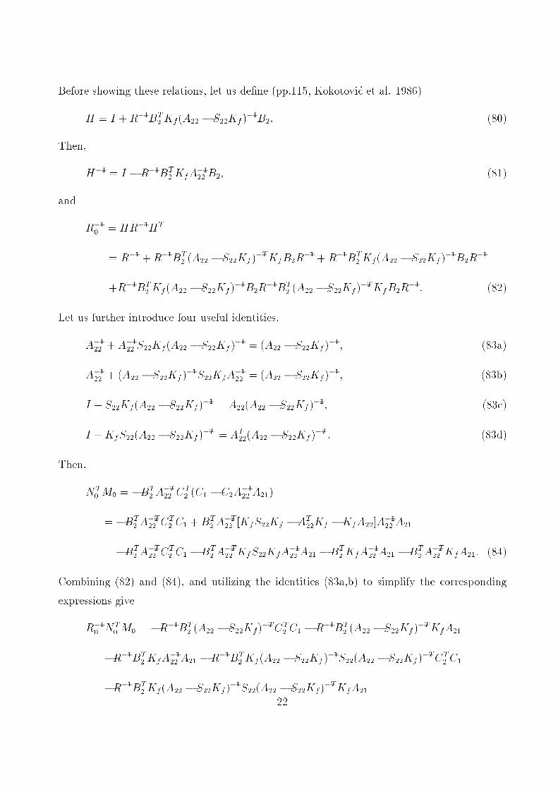
Before showing these relations, let us de�ne (pp.115, Kokotovi�c et al. 1986)
H = I +R�1BT2 Kf (A22 � S22Kf )
�1B2: (80)
Then,
H�1 = I �R�1BT2 KfA
�122 B2; (81)
and
R�10 = HR�1HT
= R�1 +R�1BT2 (A22 � S22Kf )
�TKfB2R�1 + R�1BT
2 Kf(A22 � S22Kf )�1B2R
�1
+R�1BT2 Kf (A22 � S22Kf)
�1B2R�1BT
2 (A22 � S22Kf)�TKfB2R
�1: (82)
Let us further introduce four useful identities.
A�122 + A�122 S22Kf(A22 � S22Kf )�1 = (A22 � S22Kf )
�1; (83a)
A�122 + (A22 � S22Kf )�1S22KfA
�122 = (A22 � S22Kf )
�1; (83b)
I + S22Kf(A22 � S22Kf )�1 = A22(A22 � S22Kf )
�1; (83c)
I +KfS22(A22 � S22Kf )�T = AT
22(A22 � S22Kf )�T : (83d)
Then,
NT0 M0 = �BT
2 A�T22 C
T2 (C1 � C2A
�122 A21)
= �BT2 A
�T22 C
T2 C1 +BT
2 A�T22 [KfS22Kf � AT
22Kf �KfA22]A�122 A21
= �BT2 A
�T22 C
T2 C1 �BT
2 A�T22 KfS22KfA
�122 A21 �BT
2 KfA�122 A21 �BT
2 A�T22 KfA21: (84)
Combining (82) and (84), and utilizing the identities (83a,b) to simplify the corresponding
expressions give
R�10 NT0 M0 = �R�1BT
2 (A22 � S22Kf)�TCT
2 C1 �R�1BT2 (A22 � S22Kf )
�TKfA21
�R�1BT2 KfA
�122 A21 �R�1BT
2 Kf (A22 � S22Kf )�1S22(A22 � S22Kf )
�TCT2 C1
�R�1BT2 Kf (A22 � S22Kf)
�1S22(A22 � S22Kf)�TKfA21
22
�R�1BT2 Kf (A22 � S22Kf)
�1S22KfA�122 A21: (85)
Hence,
A0 �B0R�10 NT
0 M0 = A11 � A12A�122 A21 � [B1 � A12A
�122 B2]�
[�R�1BT2 (A22 � S22Kf )
�TCT2 C1 �R�1BT
2 (A22 � S22Kf)�TKfA21
�R�1BT2 KfA
�122 A21 �R�1BT
2 Kf (A22 � S22Kf )�1S22(A22 � S22Kf )
�TCT2 C1
�R�1BT2 Kf (A22 � S22Kf)
�1S22(A22 � S22Kf)�TKfA21
�R�1BT2 Kf (A22 � S22Kf)
�1S22KfA�122 A21]
= A11 � A12(A22 � S22Kf)�1A21 + S12Kf (A22 � S22Kf)
�1A21
+S12(A22 � S22Kf )�TCT
2 C1 + S12(A22 � S22Kf)�TKfA21
+S12Kf (A22 � S22Kf)�1S22(A22 � S22Kf )
�TCT2 C1
+S12Kf (A22 � S22Kf)�1S22(A22 � S22Kf )
�TKfA21
�A12(A22 � S22Kf)�1S22(A22 � S22Kf)
�TCT2 C1
�A12(A22 � S22Kf)�1S22(A22 � S22Kf)
�TKfA21; (86)
where, the identities (83a,b) have also been used to simplify the expressions. After expanding
As of (30b), we arrive at the conclusion that As is the same as (86), which proves (79a). Now,
considering (79b), we have
B0H = (B1 � A12A�122 B2)[I +R�1BT
2 Kf (A22 � S22Kf)�1B2]
= B1 + S12Kf (A22 � S22Kf )�1B2 � A12[A
�122 + A�122 S22Kf(A22 � S22Kf )
�1]B2
= B1 + S12Kf (A22 � S22Kf )�1B2 � A12(A22 � S22Kf )
�1B2
= B1 � (A12 � S12Kf )(A22 � S22Kf)�1B2
= B1 +N1sB2: (87)
23
Therefore,
B0R�10 BT
0 = B0HR�1HTBT0
= (B1 +N1sB2)R�1(B1 +N1sB2)
T
= BsR�1BT
s = Ss; (88)
which proves (79b). Finally,
�MT0 N0R
�10 NT
0 M0 =
[�CT1 C2A
�122 B2 � AT
21KfA�122 B2 � AT
21A�T22 KfB2 + AT
21A�T22 KfS22KfA
�122 B2]
�[R�1BT2 (A22 � S22Kf )
�TCT2 C1 +R�1BT
2 (A22 � S22Kf )�TKfA21
+R�1BT2 KfA
�122 A21 +R�1BT
2 Kf (A22 � S22Kf)�1S22(A22 � S22Kf )
�TCT2 C1
+R�1BT2 Kf(A22 � S22Kf )
�1S22(A22 � S22Kf)�TKfA21
+R�1BT2 Kf(A22 � S22Kf )
�1S22KfA�122 A21]
= �CT1 C2A
�122 S22(A22 � S22Kf )
�TCT2 C1 � CT
1 C2A�122 S22(A22 � S22Kf)
�TKfA21
�CT1 C2A
�122 S22Kf (A22 � S22Kf)
�1S22(A22 � S22Kf )�TCT
2 C1
�CT1 C2A
�122 S22Kf (A22 � S22Kf)
�1S22(A22 � S22Kf )�TKfA21
�CT1 C2A
�122 S22KfA
�122 A21 � CT
1 C2A�122 S22Kf(A22 � S22Kf )
�1S22KfA�122 A21
�AT21KfA
�122 S22(A22 � S22Kf )
�TCT2 C1 � AT
21KfA�122 S22(A22 � S22Kf )
�TKfA21
�AT21KfA
�122 S22KfA
�122 A21
�AT21KfA
�122 S22Kf (A22 � S22Kf )
�1S22(A22 � S22Kf )�TCT
2 C1
�AT21KfA
�122 S22Kf (A22 � S22Kf )
�1S22(A22 � S22Kf )�TKfA21
�AT21KfA
�122 S22Kf (A22 � S22Kf )
�1S22KfA�122 A21
�AT21A
�T22 KfS22(A22 � S22Kf)
�TCT2 C1 � AT
21A�T22 KfS22(A22 � S22Kf)
�TKfA21
24

�AT21A
�T22 KfS22Kf(A22 � S22Kf )
�1S22(A22 � S22Kf)�TCT
2 C1
�AT21A
�T22 KfS22Kf(A22 � S22Kf )
�1S22(A22 � S22Kf)�TKfA21
�AT21A
�T22 KfS22KfA
�122 A21 � AT
21A�T22 KfS22Kf (A22 � S22Kf)
�1S22KfA�122 A21
+AT21A
�T22 KfS22KfA
�122 S22(A22 � S22Kf )
�TCT2 C1
+AT21A
�T22 KfS22KfA
�122 S22(A22 � S22Kf )
�TKfA21
+AT21A
�T22 KfS22KfA
�122 S22(A22 � S22Kf )
�TKfA21
+AT21A
�T22 KfS22KfA
�122 S22Kf (A22 � S22Kf )
�1S22(A22 � S22Kf )�TCT
2 C1
+AT21A
�T22 KfS22KfA
�122 S22Kf (A22 � S22Kf )
�1S22(A22 � S22Kf )�TKfA21
+AT21A
�T22 KfS22KfA
�122 S22Kf (A22 � S22Kf )
�1S22KfA�122 A21: (89)
Using the identities of (83), (89) reduces to
�MT0 N0R
�10 NT
0 M0 =
�CT1 C2(A22 � S22Kf )
�1S22(A22 � S22Kf )�TCT
2 C1
�CT1 C2(A22 � S22Kf )
�1S22(A22 � S22Kf )�TKfA21
�CT1 C2(A22 � S22Kf )
�1S22KfA�122 A21
�AT21Kf(A22 � S22Kf )
�1S22(A22 � S22Kf)�TCT
2 C1
�AT21Kf(A22 � S22Kf )
�1S22(A22 � S22Kf)�TKfA21
�AT21Kf(A22 � S22Kf )
�1S22KfA�122 A21
�AT21A
�T22 KfA22(A22 � S22Kf )
�1S22(A22 � S22Kf )�TCT
2 C1
�AT21A
�T22 KfA22(A22 � S22Kf )
�1S22(A22 � S22Kf )�TKfA21
�AT21A
�T22 KfA22(A22 � S22Kf )
�1S22KfA�122 A21
+AT21A
�T22 KfS22Kf (A22 � S22Kf )
�1S22(A22 � S22Kf )�TCT
2 C1
25

+AT21A
�T22 KfS22Kf (A22 � S22Kf )
�1S22(A22 � S22Kf )�TKfA21
+AT21A
�T22 KfS22Kf (A22 � S22Kf )
�1S22KfS22KfA�122 A21
= �CT1 C2(A22 � S22Kf )
�1S22(A22 � S22Kf )�TCT
2 C1
�CT1 C2(A22 � S22Kf )
�1S22(A22 � S22Kf )�TKfA21
�CT1 C2(A22 � S22Kf )
�1S22KfA�122 A21
�AT21Kf(A22 � S22Kf )
�1S22(A22 � S22Kf)�TCT
2 C1
�AT21Kf(A22 � S22Kf )
�1S22(A22 � S22Kf)�TKfA21
�AT21Kf(A22 � S22Kf )
�1S22KfA�122 A21
�AT21A
�T22 KfS22(A22 � S22Kf)
�TCT2 C1
�AT21A
�T22 KfS22(A22 � S22Kf)
�TKfA21
�AT21A
�T22 KfS22KfA
�122 A21: (90)
Therefore,
MT0 M0 �MT
0 N0R�10 NT
0 M0 =
CT1 C1 � AT
21A�T22 C
T2 C1 � CT
1 C2A�122 A21
+AT21A
�T22 [�KfA22 � AT
22Kf +KfS22Kf ]A�122 A21
�CT1 C2(A22 � S22Kf )
�1S22(A22 � S22Kf )�TCT
2 C1
�CT1 C2(A22 � S22Kf )
�1S22(A22 � S22Kf )�TKfA21
�CT1 C2(A22 � S22Kf )
�1S22KfA�122 A21
�AT21Kf(A22 � S22Kf )
�1S22(A22 � S22Kf)�TCT
2 C1
�AT21Kf(A22 � S22Kf )
�1S22(A22 � S22Kf)�TKfA21
�AT21Kf(A22 � S22Kf )
�1S22KfA�122 A21
26

�AT21A
�T22 KfS22(A22 � S22Kf)
�TCT2 C1
�AT21A
�T22 KfS22(A22 � S22Kf)
�TKfA21
�AT21A
�T22 KfS22KfA
�122 A21
= CT1 C1 � AT
21(A22 � S22Kf )�TCT
2 C1 � CT1 C2(A22 � S22Kf)
�1A21
�CT1 C2(A22 � S22Kf )
�1S22(A22 � S22Kf )�TCT
2 C1
�CT1 C2(A22 � S22Kf )
�1S22(A22 � S22Kf )�TKfA21
�AT21Kf(A22 � S22Kf )
�1S22(A22 � S22Kf)�TCT
2 C1
�AT21Kf(A22 � S22Kf )
�1S22(A22 � S22Kf)�TKfA21
�AT21Kf(A22 � S22Kf )
�1A21 � AT21(A22 � S22Kf )
�TKfA21: (91)
On the other hand, expanding Qs of (30a) and noting Kf = P+22s lead to the conclusion that Qs
is the same as (91), which proves (79c). In consequence, we have Ks = P+11s, hence, K
Tm = P+
21s.
The proof of Theorem 4 is completed. ■
References
Bender, D. J. and A.J. Laub (1987a). The linear-quadratic optimal regulator for descriptor
systems. IEEE Transactions on Automatic Control, AC-32, 672-688.
Bittanti, S., A.J. Laub, and J.C. Willems (1991). Eds. The Riccati Equation. Springer-
Verlag, New York.
Chow, J. H. and P. V. Kokotovic (1976). A decomposition of near-optimum regulators for
systems with slow and fast modes. IEEE Transactions on Automatic Control, AC-21,
701-705.
Dai, L. (1989). Singular Control Systems. Lecture Notes in Control and Information Sciences,
Edited by M.Thoma and A.Wyner, Springer-Verlag, Berlin.
27
Dieudonn�e, J. (1982). Treatise on Analysis, Vol.III. Academic Press, New York.
Gajic, Z. and X. Shen (1993). Parallel Algorithms for Optimal Control of Large Scale Linear
Systems. Springer-Verlag, London.
Khalil, H. K. (1989). Feedback control of nonstandard singularly perturbed systems. IEEE
Transactions on Automatic Control, AC-34, 1052-1060.
Kokotovic, P. V., H. K. Khalil, and J. O'Reilly (1986) Singular Perturbation Methods in
Control: Analysis and Design. Academic Press, New York.
Lancaster, P. and M. Tismenetsky (1985). The Theory of Matrices. Academic Press, New
York.
Pan, Z. and T. Ba�sar (1993). H1-optimal control for singularly perturbed systems. Part I:
Perfect state measurements. Automatica, 29, 401-423.
Wang, Y.Y., S.J. Shi and Z.J.Zhang (1988). A descriptor-system approach to singular pertur-
bation of linear regulators. IEEE Transactions on Automatic Control, AC-33, 370-373.
Wang, Y. Y. and P. M. Frank (1992). Complete decomposition of sub-optimal regulator for
singularly perturbed systems. International Journal of Control, 55, 49-60.
Wang, Y. Y., P. M. Frank and D. J. Clements (1993). The robustness properties of the linear
quadratic regulators for singular systems. IEEE Transactions on Automatic Control,
AC-38, 96-100.
Wang, Y. Y., P. M. Frank and N. E. Wu (1994). Near-optimal control of nonstandard
singularly perturbed systems. Automatica, 30, 277-292.
Xu, H. and K. Mizukami (1993). Hamilton-Jacobi equation for descriptor systems. System
& Control Letter, 21, 321-327.
Xu, H. and K. Mizukami (1994). The linear-quadratic optimal regulator for continuous-time
descriptor systems: a dynamic programming approach. International Journal of Systems
Sciences, 25, 1889-1998.
28