Path Loss Parameters in Wi-Fi Networks

Date: Dec 21st , 2007

Authors:

Marufur Rahman, <100666890>, <mrahman2080@hotmail.com>

1. Introduction:

1.1 Context/Background

Traditional network security is tough enough, but with wireless networks such as

Wi-Fi, the very nature of the medium is a hacker’s dream come true. The open

air around us carries the radio signals with few restrictions, and this peculiarity of

wireless networks makes them vulnerable to stealth attackers camouflaging their

location to avoid detection and retribution. But it’s possible to track down these

hackers by the clues they leave behind: the strength of their transmission signal

when it is received by other devices.

The first goal of this project was to conduct an outdoor experiment on campus to

examine the signal propagation characteristics of a mobile device. The data

collected from this experiment helped to determine if the mobile device’s location

could be pinpointed from the received signal strength.

The second goal was to correlate the experimental data using linear regression

techniques to determine the signal propagation path loss parameters

1.2 Definition of the problem

The first goal of this project was to conduct an outdoor experiment on campus to

examine the signal propagation characteristics of a mobile device. The data

collected from this experiment helped to determine if the mobile device’s location

could be pinpointed from the received signal strength.

The second goal was to correlate the experimental data using linear regression

techniques to determine the signal propagation path loss parameters.

1.3. Summary of the result

The result of this project presents a document explaining the graphs created

from the data sent by the broadcast utility and captured by wireshark.

1.4 Outline of the report

Detailed background information about the hardware and software required is

provided in Section 2. The development setup is reviewed in Section 3. The

results of this work are presented in Section 4. The results of the project

execution are presented in Section 5. The contributions of each team member in

this project are described in Section 6.

2. Detailed context/background information:

Wi-Fi

Wi-Fi, also unofficially known as Wireless Fidelity, is a wireless technology brand

owned by the Wi-Fi Alliance intended to improve the interoperability of wireless

local area network products based on the IEEE 802.11 standards.

Common applications for Wi-Fi include Internet and VoIP phone access, gaming,

and network connectivity for consumer electronics such as televisions, DVD

players, and digital cameras.

Path Loss

When a computer sends a packet it sends it with specific signal strength, but at

the receiver end the original signal strength is reduced to some lower signal

strength. This loosing of strength refers to path loss. The goal of this project is

to do an experiment to find a relation between path loss and position of the

computers sending the signal.

3. Development setup:

3.1 Required Equipments

For this project we used four desktop computers with special network cards

which can talk to wireshark software and a laptop computer.

3.2 WireShark

Wireshark (formerly known as Ethereal) is a free software protocol analyzer, or

"packet sniffer" application, used for network troubleshooting, analysis, software

and protocol development, and education. It has all of the standard features of a

protocol analyzer.

The functionality Wireshark provides is very similar to tcpdump, but it has a GUI

front-end, and many more information sorting and filtering options. It allows the

user to see all traffic being passed over the network (usually an Ethernet

network but support is being added for others) by putting the network card into

promiscuous mode.

Wireshark is a software that "understands" the structure of different network

protocols. Thus it's able to display encapsulation and single fields and interpret

their meaning. Wireshark uses pcap to capture packets, so it can only capture on

networks supported by pcap.

3.3 Simulation

The plan is to set those 5 machines in a common place where internet access is

available in school (The quad seemed perfect for that). Before we start we have

to make sure all the desktops has wireshark up and running. Then we have to

filter the capture packets only from our source (the Laptop). We have to then

place the desktops in four corners of the quad. Then one has to take the laptop

and stand somewhere in between those corners and we have to measure the

distances from the laptop to the desktops (as we need the distances to correlate

the data). Then we have to send packets (browse internet) from the laptop for

certain period (5 minutes) and change the position of the laptop and do the

same thing again. In the mean time we have to save those data in wireshark in a

dump file which will later be used to correlate. Once we get all those data from

5- 10 repetitions of the experiment we will process those dump files to some java

readable format, and using java we will make a graphics representation of linear

regression.

3.4 Broadcast Utility

From the laptop thousands of broadcast messages were sent using a utility

which uses UDP to do that. The simple C program opens a socket and sends

thousands of broadcast packets over UDP and closes the socket once it’s done

sending packets. The program is as follow.

#include <winsock.h>#include <stdio.h>

main()

{

WSADATA ws;WSAStartup(0x0101,&ws);int i;

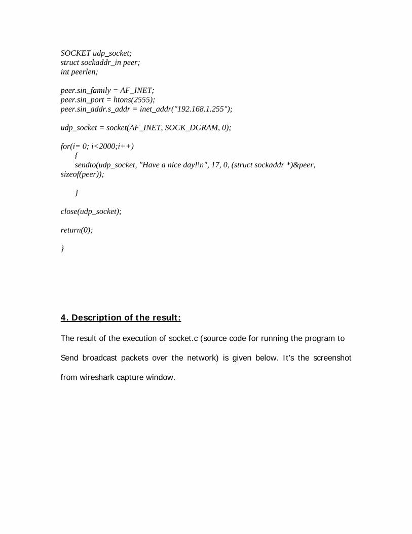
SOCKET udp_socket;struct sockaddr_in peer;int peerlen;

peer.sin_family = AF_INET;peer.sin_port = htons(2555);peer.sin_addr.s_addr = inet_addr("192.168.1.255");

udp_socket = socket(AF_INET, SOCK_DGRAM, 0);

for(i= 0; i<2000;i++) { sendto(udp_socket, "Have a nice day!\n", 17, 0, (struct sockaddr *)&peer, sizeof(peer)); }

close(udp_socket);

return(0);

}

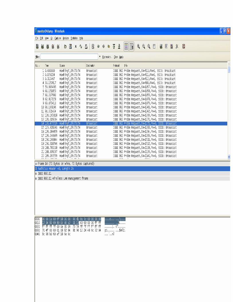
4. Description of the result:

The result of the execution of socket.c (source code for running the program to

Send broadcast packets over the network) is given below. It’s the screenshot

from wireshark capture window.

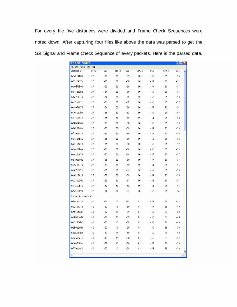
For every file five distances were divided and Frame Check Sequences were

noted down. After capturing four files like above the data was parsed to get the

SSI Signal and Frame Check Sequence of every packets. Here is the parsed data.

This data table shows the different distances and relevant SSI Signal strength of

every packets matched by the frame check sequence number of each packets.

4.1 Linear Regression

The captured data for every monitor was used to use linear regression technique

to find the best fit for n where

path loss = path loss at d0 + 10*n*log10(d/d0)

where d0 is our reference distance .001 Km(1m), and d = relevant distance.and

path loss at d0 in free space = 32.45 + 20*log10(f) + 20*log10(d0)

where f is the frequency expressed in MHz ,and for our wifi experiment it was

2.4 GHz= 2400 MHz. After putting the values for f and d0 we get

path loss at d0 in free space = 40.05.

After that all the theoretical pathlosses were drawn against the relevant

distances for each monitor separately and one with all the monitor’s pathloss was

drawn too. We considered n=1, 2, 3, 4, 5 as those values cover all the points in

the graph. Below is a sample of representation of the graphs which were drawn

from the data taken for every desktop separately. This graph represents the

distance and path loss (SSI Signal strength) co-relation while horizontal bar

represents log of each distances for a certain desktop and vertical bar represents

the path loss (17db- actual SSI Signal captured live).

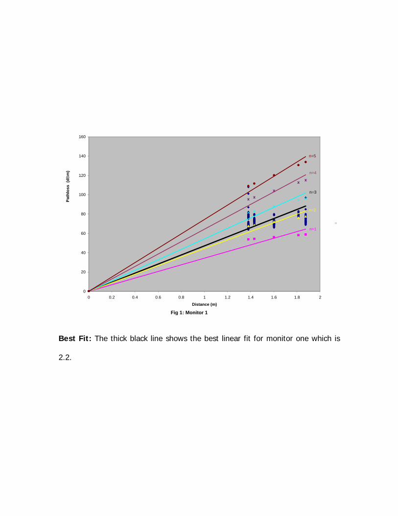
Fig 1: Monitor 1

n=1

n=2

n=3

n=4

n=5

0

20

40

60

80

100

120

140

160

0 0.2 0.4 0.6 0.8 1 1.2 1.4 1.6 1.8 2

Distance (m)

Pat

hlo

ss

(dB

m)

Best Fit: The thick black line shows the best linear fit for monitor one which is

2.2.

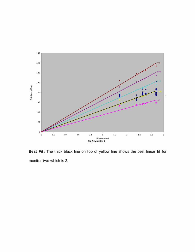
Fig2: Monitor 2

n=1

n=2

n=3

n=4

n=5

0

20

40

60

80

100

120

140

160

0 0.2 0.4 0.6 0.8 1 1.2 1.4 1.6 1.8 2

Distance (m)

Pat

hlo

ss (

dB

m)

Best Fit: The thick black line on top of yellow line shows the best linear fit for

monitor two which is 2.

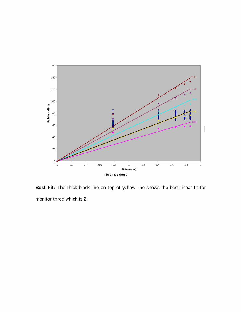
Fig 3 : Monitor 3

n=1

n=2

n=3

n=4

n=5

0

20

40

60

80

100

120

140

160

0 0.2 0.4 0.6 0.8 1 1.2 1.4 1.6 1.8 2

Distance (m)

Pat

hlo

ss (

dB

m)

Best Fit: The thick black line on top of yellow line shows the best linear fit for

monitor three which is 2.

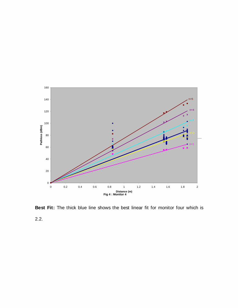
Fig 4 : Monitor 4

n=1

n=2

n=3

n=4

n=5

0

20

40

60

80

100

120

140

160

0 0.2 0.4 0.6 0.8 1 1.2 1.4 1.6 1.8 2

Distance (m)

Pat

hlo

ss

(d

Bm

)

Best Fit: The thick blue line shows the best linear fit for monitor four which is

2.2.

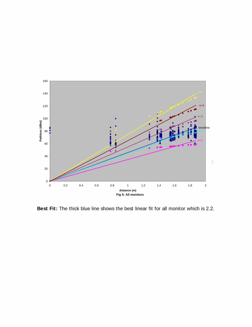
Fig 5: All monitors

trendline

n=1

n=5

n=2

n=3

n=4

0

20

40

60

80

100

120

140

160

0 0.2 0.4 0.6 0.8 1 1.2 1.4 1.6 1.8 2

distance (m)

Pa

thlo

ss (

dB

m)

Best Fit: The thick blue line shows the best linear fit for all monitor which is 2.2.

5. Evaluation of the result:

The graph drawn from the data captured suggests that there is a definite co-

relation between the distance and the signal strength of the transmission. The

thick black line in figure 5 shows the best linear regression fit to the data and

indicates that average wifi path loss increases as distance to the power 2.2. This

best fit was found by using least square method on the data captured for every

distance for every monitor. So we could conclude saying that it is possible to

track down a hacker’s location from the clue he leaves behind, SSI Signal

strength.

6. Contributions of team member:

Marufur Rahman wrote the broadcast utility, Set up all those desktops to capture

data sent by the utility, parsed the data and represented the graph.

7. Acknowledgement:

I would love to convey my sincere appreciation to Dr Michel Barbeau for inspiring

me to find this interesting open topic and providing all necessary assistance.

I thank Chirtine Laurendeau, a PhD In Carleton who was also the co-supervisor

of the project .I would also like to thank Chen Guang Lee (a Master’s student at

carleton university) and my intimate friends for giving me continuous supports

8. References:

[1] Wireshark Tutorial. http://www.wireshark.org, 2007.

[2] Wikipedia. http://www.wikipedia.org, 2007