TOPIC 5: CAPITAL STRUCTURE AND THE PRODUCT MARKET

1. Introduction

Traditionally, the strategy of the firm in the product market and its financial strategy were studied in

isolation: the industrial organization literature that studies the strategies of the firm in the product market,

has ignored the financial structure of the firm, while the corporate finance literature that studies the

financial strategies of the firm in the capital market has ignored the strategies of the firm in the product

market. Specifically, the maintained assumption in industrial organization literature is that firms are all-

equity, and the maintained assumption in the corporate finance literature is that the earnings of firms come

from a black-box and are represented by some prespecified distribution. Recently, a small but growing

literature has emerged which tries to bridge this gap and explore the interaction between these two

literatures. In this chapter we shall review the main contributions to this literature and we shall see that

this new literature has uncovered interesting and important linkages between financial strategies and

competitive strategies. This suggests that one cannot study the financial and "real" aspects of the firm’s

operations in isolation as this approach involves a serious loss of insights.

2. The interaction between debt and competition in the product market

One of the first papers to explore the linkage between capital structure and competition in the product

market, and probably the most important one in this area to date is "Oligopoly and Financial Structure:

The Limited Liability Effect" by Brander and Lewis (AER, 1986). This paper shows that issuing risky

debt induces firms to be more aggressive in the product market than they would otherwise be, and this

aggressive behavior may confer a strategic advantage on the firm in the product market. This effect of

risky debt can be thought of as a special form of asset substitution effect (in the asset substitution effect

2

the firm also adopts an aggressive investment behavior). But, since the firm in Brander and Lewis does

not choose the distribution of earnings as in Jensen and Meckling (which is the salient feature of the asset

substitution problem) it is probably better to think about this effect as a distinct one. Indeed, Brander and

Lewis refer to this effect of risky debt as "the limited liability effect."

The framework that Brander and Lewis adopt is the traditional Cournot model that is so familiar

from intermediate micro textbooks. In this model there are two firms that produce a homogenous good.

The firms choose simultaneously their respective output levels and given these quantities, the price of the

good is determined in the product market according to the demand curve. As is well-known, quantities

in the Cournot model are strategic substitutes: when firm 1 becomes more aggressive, firm 2 becomes

softer, and vice versa.1 This result is due to the fact that the reaction curves or best-response functions

of the two firms are downward sloping in the strategy space. This feature of the model implies that it is

beneficial for each firm to commit itself to an aggressive behavior in the product market by adopting a

strategy that will shift its reaction curve outward (i.e., commit the firm to produce a larger quantity for

each quantity produced by the rival). There is a vast literature in industrial organization (see the

references in Shapiro or in Tirole) that shows how firms can use different strategies to commit to an

aggressive behavior. Brander and Lewis show that issuing risky debt is another way to commit a firm

to an aggressive behavior in the product market.

To establish the limited liability effect, Brander and Lewis add to the traditional Cournot model

two features. First, they assume that there is some random shock that affects the operating profits of the

two firms either through the demand for the good or either through the cost function. Second, they

assume that each firm may issue debt before it decides how much it wants to produce, and that each firm

is run by equityholders who care only about their own payoff and ignore the payoff of debtholders. As

1 See for example Shapiro, C. "Theories of Oligopoly Behavior." In R. Schmalensee and R. Willig,eds., Handbook of Industrial Organization. New York: North Holland, (1989), or Chapter 7 in Tirole J.The Theory of Industrial Organization. Cambridge MA: M.I.T. Press (1988).

3

we shall see below, this is important since equityholders are protected by limited liability so in the event

of bankruptcy equityholders cannot be forced to pay more than the firm earns and their payoff is zero.

Having described the main features of the model, let’s examine now the details and let’s introduce

notations. As usual, there are two periods: in period 1, the two firms choose how much debt they wish

to issue. Debt becomes due at the end of period 2. Let Di be the face value of debt issued by firm i.

In period 2, the two firms simultaneously choose their respective output levels, q1 and q2. Given a pair

of output levels and the realization of a random shock, z, the operating profits (i.e., revenues minus costs)

of the two firms are determined, R1(q1,q2,z) and R2(q1,q2,z).2 Assume without a loss of generality, that

the random shock, z, is distributed on the interval [0, 1] according to a cumulative distribution function

F(z) and density f(z). Moreover, assume that higher levels of z are associated with better states of nature

in that Rzi(.) > 0, i = 1,2, where subscripts denote partial derivatives. That is, the higher is the value of

z, the higher are the operating profits of the two firms. Finally, the operating profit is distributed to

securityholders according to their respective claims. In the event that the firm’s operating profit fall short

of the debt obligation, the firm declares bankruptcy, and equityholders, who are protected by limited

liability, receive a zero payoff, while debtholders become the residual claimants.

To solve the model, let’s assume first that the firm is all-equity. Then the firm chooses in period

2 an output level, qi, to maximize its value given by

taking the output level of its rival, qj, as given. Using subscripts to denote partial derivatives, the first

(1)

order condition for firm i’s maximization problem is:

2 Here we assume that z is a common shock but we could also assume that the two firms facepotentially different shocks, z1 and z2. This assumption however does not add anything to the analysisso we can economize on notations by assuming a common shock.

4

Equation (2) defines qi as an implicit function of qj: that is, equation (2) defines the best-response of firm

(2)

i against the strategy of firm j (recall that a strategy in the product market is a choice of quantity, so firm

j’s strategy is qj). Solving the system of two best-response functions (one for firms 1 and one for firm

2) yields a Nash equilibrium (q1*, q2*). This equilibrium is the same as the Nash equilibrium in any

traditional Cournot model except that here the best-response of firm i against the strategy of firm j is not

determined by the marginal operating profit, Rii(.), but rather by the expectation of Ri

i(.) which is taken

over all possible states of nature. In a model without a random shock, the firm produces up to the point

where its marginal operating profit is zero. Assuming that Ri(.) is concave (this assumption ensures that

the maximization problem is nicely behaved), Rii(.) is downward sloping. Thus for small qi’s, Ri

i(.) is

positive, so the firm benefits from increasing its output level. This continues until Rii(.) = 0. From that

point on, Rii(.) becomes negative so the firm does not wish to increase its output further. The same logic

applies when the firm’s operating profits are subject to a random shock but now the firm chooses an

optimal quantity by equating the expected value of Rii(.) to zero.

Now consider the case where the firm has issued debt in period 1. Given Di, there exists a critical

states of nature, zi such that the firm is just able to return its debt. Since by assumption Rzi(.) > 0, i = 1,

2, it is clear that for values of z less than zi, the firm goes bankrupt, while for value of z above zi, the firm

remains solvent. zi is defined implicitly by

and is illustrated in Figure 1. We assume here that Di always exceeds Ri(q1, q2, 0) (i.e., the operating

(3)

profit of the firm in the worst state of nature) otherwise the firm can repay it with probability 1 so debt

is riskless.

Figure 1: Determining the critical state of nature below which the firm goes bankrupt

Di

z

Ri(q1,q2,z)

zi 1

5

The objective of the firm is to maximize the value to equityholders. The market value of equity

is given by:

The right side of equation (4) represents the expected operating profits, net of debt payments, over states

(4)

of nature in which the firm remains solvent and its equityholders are the residual claimants.

To compute the best-response of firm i, note that qi affects Ei both directly through its effect on

the function Ri(.) but also indirectly because it affects zi and hence the likelihood that the firm goes

bankrupt. Differentiating Ri(.) with respect to qi, the first condition for qi is given by

The first term on the right side of equation (5) represents the effect of increased quantity on the likelihood

(5)

that the firm goes bankrupt: a small increase in output raises zi by ∂zi/∂qi and the change in equityholders

payoff in this case -[Ri(q1,q2,zi) - Di]. But, definition (3), this term vanishes implying that the indirect

effect of qi on Ei is negligible. The second term is the expected marginal operating profits over all states

of nature in which the firm remains solvent. This effect is not negligible.

Having derived the best-response of firm i it remains to show that firm i becomes more aggressive

when Di increases. To this end, note that equation (5) defines qi as an implicit function of Di. Totally

differentiating this equation yields:

where Eiii is the second derivative of Ei with respect to qi and EiDi

i is the cross-partial derivative of Ei with

(6)

respect to qi and Di. Since the second order condition for maximization requires that Eiii < 0, it is clear

6

that whether qi increases or decreases with Di depends on the sign of EiDii. If EiDi

i > 0, the marginal payoff

of equityholders increases when the firm is more leveraged, and as a result, the firm expands its

production for every level of qj and hence becomes more aggressive. If EiDii < 0, the marginal payoff of

equityholders decreases when the firm is more leveraged, so now debt induces the firm to cut its

production and become a softer competitor in the market. To determine the sign of EiDii we need to

differentiate equation (5) with respect to Di. Noting that Di affects this equation only indirectly through

its effect zi, we get:

From Figure 1 it is clear that ∂zi/∂Di > 0 since more debt means that the firm goes bankrupt in more states

(7)

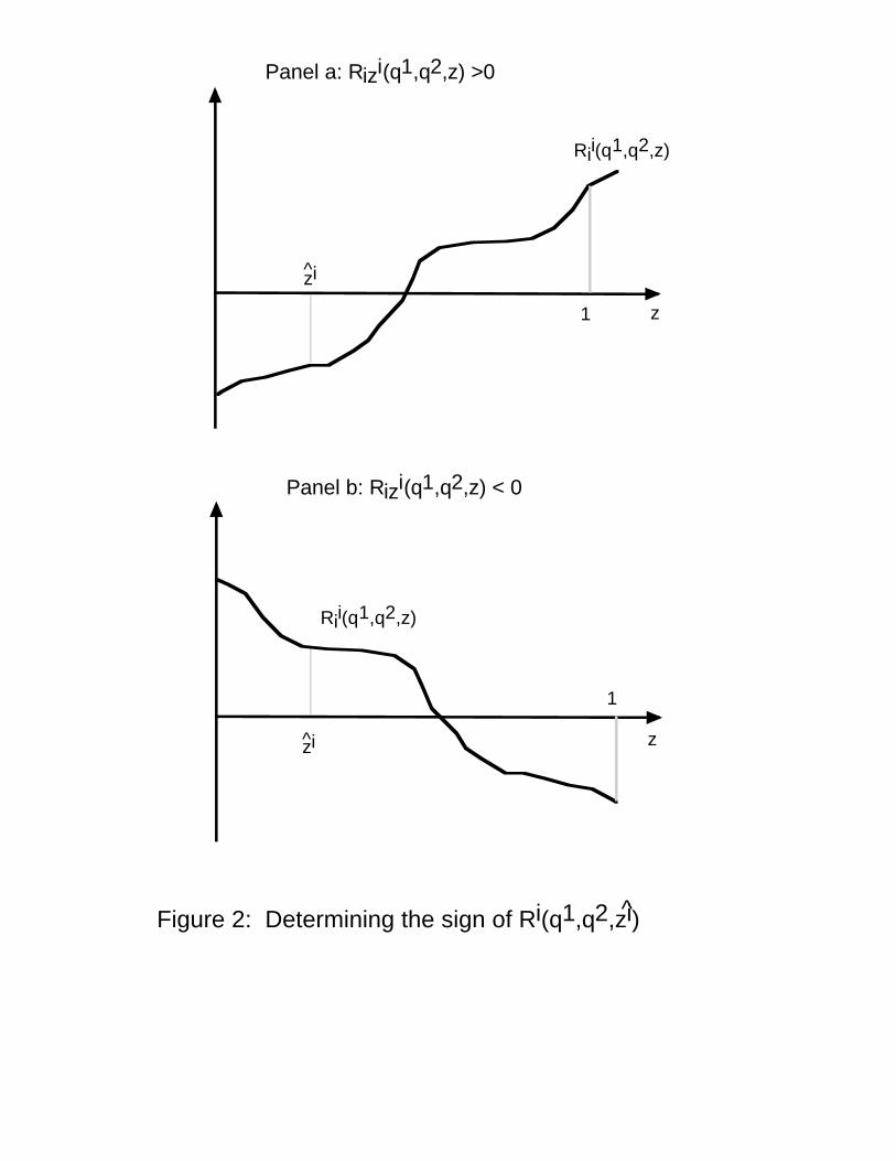
of nature. As for Rii(q1,q2,zi), we need to know whether Riz

i(.) is positive or negative. Figure 2 presents

the two possibilities. The top panel shows that case where Rizi(.) > 0. By the first order condition for qi,

the expectation of Rii(.) over all states between zi and 1 has to equal zero. Hence, Ri

i(.) has to be positive

for some z’s and negative for others. But, if Rii(.) increases with z, it is clear that Ri

i(.) is negative for

low values of z and positive for high values. Since zi is the lowest value of z that the firm takes into

account it is clear that Rii(q1,q2,zi) < 0. Therefore, equation (7) shows that ∂qi/∂Di > 0 implying that the

firm becomes more aggressive as its debt level increases. Likewise, the bottom panel in Figure 2 shows

the case where Rizi(.) < 0. Then, Ri

i(.) is positive for low values of z and negative for high values since

in expectation it has to be equal to zero. Since zi is the lowest value of z that the firm takes into account

it is clear that Rii(q1,q2,zi) > 0, so equation (7) implies that ∂qi/∂Di < 0. Therefore in the firms becomes

softer in this case when it has more debt.

Intuitively, issuing debt means that the firm ignores low states of nature in which the firm goes

bankrupt and chooses its competitive strategy, qi, by taking into account only those states in which its

remains solvent. If Rizi(.) > 0 then the marginal operating profit of the firm is higher in high states of

z

Rii(q1,q2,z)

1

zzi^

1

Figure 2: Determining the sign of Ri(q1,q2,zi)^

Rii(q1,q2,z)

zi^

Panel b: Rizi(q1,q2,z) < 0

Panel a: Rizi(q1,q2,z) >0

7

nature so the firm who takes into account only high states wishes to produce more. It simply ignores

states in which it is supposed to produce little. If Rizi(.) < 0, the reveres is true: the marginal operating

profit of the firm is lower in high states of nature so the firm who takes into account only high states

wishes to produce less as it simply ignores low states of nature in which it is supposed to produce little.

Since high values of z are associated with good states of nature in the sense that the operating profit of

the firm increases with z, this last case is not very intuitive: it says that although the firm makes more

profits, it marginal profits are lower in better states. Nonetheless, this case may arise for example, if an

increase in z leads to a significant drop in fixed cost but a small rise in variable cost. In this case, high

values of z lead to higher profits but lower marginal profits. Although the firm would earn more money

it will produce less. Since in most cases it is reasonable to assume that better states of nature mean that

the marginal operating profits are higher as well, we conclude that issuing debt commits the firm to a

more aggressive behavior than in the case where the firm is all-equity.

Thus far we have shown that issuing debt makes the firm more or less aggressive in the product

market. Does this mean that the firm will wish to issue debt? It can be shown that the answer to this

question is yes. Does this mean that the firm becomes better-off? Surprisingly, the answer to this

question is no. Although each firm benefits if it alone issues debt, in equilibrium both firms will issue

debt and will therefore play more competitive strategies than they would had they remained all-equity.

Thus, the equilibrium profits of the two firms are lower than in the all-equity case. So it might be thought

that firms are better off by remaining all-equity. But had this been the case, one of the firm could have

benefitted from issuing debt. Given that its rival is leveraged the other firm would have benefitted as well

by issuing debt so the only equilibrium must be such that both firms issue debt. The logic here is similar

to the prisoners’ dilemma: firms are better off if both of them do not issue debt but can’t resist the

temptation to do so, so eventually they end up in an equilibrium which gives them less profits than can

make otherwise.

8

3. Debt in bilateral relationships

Another motivation to issue debt arises when the firm is locked into bilateral relationships with a single

trading partner and cannot switch to another partner. Examples for bilateral relationships are the

relationship between firms and their workforce when workers have specific skills so they cannot be

replaced easily, nor can they easily alternative employers, the relationship between regulated monopolies

in telephone, electricity, natural gas, and water, and the public utility commissions that regulate them and

the relationship between the government and defense contractors. As we shall see below, the firm can

improve its bargaining position vis-a-vis its trading partner by committing itself to pay money to

debtholders. Consequently, issuing debt may benefit the firm. That is, the influence of debt on the

bargaining position of a firm vis-a-vis a trading partner is yet another force that drives the capital structure

of the firm.

The idea that an agent can improve its bargaining position and thereby increase his share in the

gains from trade by committing himself to pay to a third party was first stated in the following example

due to Schelling (1960, ch. 2, p. 24): "When one wishes to persuade someone that he would not pay him

more than $16,000 for a house that is really worth $20,000 to him, what can he do to take advantage of

the usually superior credibility of the truth over false assertion? Answer: make it true... the buyer could

make an irrevocable and enforceable bet with some third party, duly recorded and certified, according to

which he would pay for the house no more than $16,000 or forfeit $5,000." Schelling’s idea was

formalized by Green (1992), who shows that financial agreements with third parties are particularly

powerful when the third parties are silent partners, not participating in the ex post bargaining, and when

the financial agreement creates a potential conflict of interests between the agent and the third parties.

Recently, a small literature has emerged that shows that firms locked into bilateral relationships

have incentive to issue risky debt. This literature includes Sarig (mimeo, 1988) and Bronars and Deere

(QJE, 1991) who show that by issuing risky debt, a firm improve its bargaining position vis-a-vis a labor

9

union; Israel (JF, 1991) who shows that by issuing debt, an incumbent management facing a more

efficient raider is able to increase its share in the gains from takeover; Spiegel (JEMS, 1996) who show

that by issuing debt the firm receives a larger share of the gains from trading with a buyer; and Dasgupta

and Nanda (IER, 1993), Spiegel and Spulber (Rand J., 1994), and Spiegel (JRE, 1994), who show that

by issuing debt, a regulated firm induces regulators to set a higher price than they would set otherwise.

The basic model

The analysis in this section is based on Spiegel (JEMS, 1996), but it is closely related to the other models

mentioned in the previous paragraph. There is a single buyer and a single seller (the firm), both of whom

are risk neutral. The relationship between the buyer and the seller evolves in two periods: in period 1,

the two parties sign an initial procurement contract for the delivery of one unit of a good in period 2.

This contract however is incomplete in that it specifies only period 1 actions, such as how to carry out

the basic R&D and who will pay for this activity, but it remains silent about the terms of trade in period

2. After signing the contract, the firm issues debt with face value D to outsiders, due at the end of period

2 after the relationship with the buyer ends, and pays the proceeds as a dividend to equityholders.3 At

the beginning of period 2, a random variable, z, that affects the relationship is realized and observed by

both parties. Then, the parties engage in an ex post bargaining in which they decide whether or not to

trade and at what price. Conditional on the bargaining outcome, payoffs are realized.

Contractual incompleteness means that each party behaves opportunistically in period 2 by

demanding a larger share as possible of the total surplus. The assumption that the parties cannot sign an

initial long-term contract can have at least two interpretations. First, the buyer may be sovereign, e.g.,

a foreign government, and may not be forced to comply with his contractual obligations, in which case,

3 If the firm raises money from outsiders and keeps the money in the firm, then it can pay it backfor sure and therefore such debt is not risky and cannot affect the analysis.

10

there is no point in having a long-term contract.4 Second, the random variable, z, may be non-verifiable

to third parties (e.g., courts) so the parties may be unable to condition the terms of trade in the contract

on z.

Let v(z) be the buyer’s valuation of the good and c(z) be the firm’s production cost, as functions

of the random variable, z. Assume that z is distributed uniformly over the unit interval. Define, V(z) ≡

v(z)-c(z), as the net valuation of the good, and assume that Vz(z) > 0, where subscripts denote partial

derivatives. The last assumption means that higher values of z represent better states of nature. For

simplicity, assume that V(0) = 0, so trade is beneficial even in the lowest state of nature.

Throughout, information is symmetric: both the buyer and the firm observe z before they engage

in the ex post bargaining. Therefore, it is natural to assume that the ex post bargaining has the following

two properties. First, the good is produced and traded if and only if the sum of the parties’ payoffs if they

trade exceeds the sum of their payoffs absent trade. Second, the buyer’s payment when trade occurs is

chosen to divide the surplus from trade between the buyer and the firm in proportions γ and 1-γ,

respectively, where γ ∈ (0, 1). The parameter γ (1-γ) is a measure of the buyer’s (firm’s) bargaining

power. The larger γ is the more powerful the buyer becomes so the contractual incompleteness becomes

more problematic from the firm’s perspective.

For simplicity, the buyer’s payoff absent trade is normalized to zero. Similarly, if the parties do

not trade, the firm makes zero profits; consequently, the firm cannot pay its debt and goes bankrupt as

a result. Since equityholders are protected by limited liability, their payoff in the event of bankruptcy is

zero. Assuming that firm acts only on behalf of equityholders, its payoff if there is no trade is therefore

zero. When the parties trade, they generate a surplus of V(z), but since D is paid to debtholders, the joint

payoff of the buyer and the firm is they trade is V(z) - D. Since the joint payoff of the parties absent

4 Other examples for sovereign parties include regulatory commissions in the U.S. who cannotcommit to long term regulated prices, and labor unions in the U.K. who cannot commit themselves toprovide future labor at an agreed rate even if they wish.

11

trade is 0, trade takes place in period 2 if and only if V(z) - D ≥ 0. This condition defines critical state

of nature, z at which the parties begin to trade and the firm is just able to repay its debt. Since Vz(z) >

0, the parties do not trade and the firm goes bankrupt when z < z, while when z ≥ z, the parties trade and

the firm remains solvent. z is defined implicitly by

Since V(0) = 0, debt is risky: the firm faces a positive probability of bankruptcy even if it has issued only

(1)

one dollar of debt. Since z is distributed uniformly over the unit interval, the probability of trade is 1-z.

This probability decreases with D since ∂(1-z)/∂D = -1/Vz(z) < 0.

Note that the ex post bargaining is inefficient since the parties forgo a surplus of V(z) whenever

D > V(z). This inefficiency is a special case of Myers’ debt overhang problem: when D > V(z), the firm

cannot repay its debt in full even if it captures V(z) entirely, so bankruptcy is unavoidable. Since

equityholders are protected by limited liability, their payoff in this case is zero regardless of whether trade

occurs, so the firm, who acts on their behalf, has no incentive to trade. This suggests that by issuing debt,

the firm can become more aggressive in the ex post bargaining, since it can credibly threaten the buyer

that it will not trade unless its share in the gains from trade is large enough to ensure that it remains

solvent.

Before continuing, it is important to emphasize that debt can serve as a credible threat only if it

is hard to restructure it.5 One way to achieve this is by issuing debt in the form of publicly traded bonds

which are typically held by a large number of relatively small individual investors, so in the event that

5 The idea that the possibility of renegotiation undermines the strategic value of agreements with thirdparties has been first stated in Schelling (1960) and was recently examined by Katz (Rand J., 1991). Todemonstrate it in the present context, suppose that debt is easy to restructure. Then, if the buyer insistson not paying more than x < D, debtholders would benefit from reducing their claims to slightly belowx to ensure that the firm remains solvent and trades. The resulting payoff of debtholders would then bex, rather than 0, which is their payoff when the firm goes bankrupt. Consequently, the firm would captureonly x of the gains from trade instead of V(k,z).

12

V(z) < D, each investor benefits from letting others forgive some of their claims. Such a free rider

problem, in turn, can impede successful restructuring.6 A second advantage of publicly traded bonds is

that they are readily observable. Without observability, agreements with third parties may not serve as

precommitments (Katz, JF, 1991). Also, note that the assumption that the firm acts on behalf of

equityholders alone is crucial for debt to be an effective threat. Otherwise, the firm will not refuse to

trade when V(z) < D, so debt will not serve as a credible threat against the buyer. Thus, equityholders

have an incentive to ensure that management’s payoff is aligned with theirs, say by tying management’s

compensation to the value of equity.7

Assuming that the capital market is perfectly competitive, the firm’s debt is fairly priced, in the

sense that the expected return of debtholders is equal to the risk free rate of return, which is normalized

for simplicity to zero. Assume that when the firm goes bankrupt, its operations are interrupted to the point

where it cannot trade with the buyer and it is therefore liquidated.8 Therefore, the market value of debt

is

6 Even in the absence of a free rider problem, a restructuring of publicly traded debt is still extremelyhard since Section 316(b) of the Trust Indenture Act of 1939 requires a unanimous debtholder consentbefore the firm can alter any core term (e.g., principal, interest, or maturity date) of a bond issue. For amodel that explicitly examines the difficulties of restructuring public debt, see Gertner and Scharfstein (JF,1991).

7 For this scheme to work, it must be also assumed that management cares only about monetarycompensation (e.g., it does not draw utility from trading per-se) and that it cannot be bribed by the buyer(e.g., bribes can result in severe punishments if detected). Also, note that managerial compensation alone(without debt), may not be sufficient to commit the firm to an aggressive position in the ex postbargaining, since it is typically easy to renegotiate and hard to observe.

8 This assumption does not entail any serious loss of generality since the same results will hold ifdebtholders can reorganize the firm at a cost after bankruptcy and resume trade with the buyer.

13

This expression describes the value of debt for relatively high values of z (z ≥ z) in which case trade takes

(2)

place debtholders are paid in full. Otherwise, no trade takes place, the firm is liquidated, and debtholders

receive a payoff of 0.

To compute the equityholders’ payoff, recall that the ex post gains from trade when it occurs, V(z)

- D, are divided between the buyer and the firm according to their respective bargaining powers, γ and

1-γ. Thus, the payoff of equityholders in period 2 when trade occurs, is (1-γ)(V(z)-D). In addition,

equityholders receive in period 1 a payoff of B(D), so their overall expected payoff as a function of the

level of investment and the face value of debt is

Debt has two effects on payoff of equityholders. First, it reduces the probability of trade from 1 to 1-z.

(3)

This reduction is the cost of debt in this model. Second, debt reduces the ex post gains from trade to be

bargained over with the buyer by D. This translates to an expected loss of D(1-z), and equityholders’

share in this expected loss is (1-γ)D(1-z). But, when debtholders buy the firm’s debt in period 1, they pay

for it B(D), so the overall change in the expected payoff of equityholders is B(D)-(1-γ)D(1-z), or γD(1-z)

which is the second term on the third line of equation (3). Thus, by committing D to debtholders,

equityholders increase their overall share in the expected gains from trade when it occurs. This increase

14

is the benefit of debt in this model.9

Anticipating the outcome of the ex post bargaining with the buyer, the firm chooses in period 1

the face value of debt to maximize Y(D). Let D* be the equilibrium financial strategy of the firm. The

first order condition for D* is given by

where dz/dD = 1/Vz(z) > 0. But, from (1) we know that V(z) = D. Hence, we can write the first order

(4)

condition for D* as

The left side of the equation is the marginal benefit of debt associated with the increase in the

(5)

equityholders share in the surplus due to debt. The right side is the marginal cost of debt associated with

the decrease in the likelihood of debt. In equilibrium, D* > 0 since at D = 0, the marginal benefit of debt

is positive (equal to γ) while the marginal cost is 0. Hence the firm always benefits from raising D

beyond 0. It is easy to see that D* increases with γ implying that the higher is the buyer’s bargaining

power, the more debt will the firm issue. The intuition for this is that the firm needs debt to shield itself

from the buyer’s opportunism, so the more opportunistic the buyer becomes, the more debt the firm needs.

At the extreme when γ = 0, the buyer is not opportunistic, so the firm captures the entire surplus and

hence does not benefit from issuing debt.

The model just described fits the situation in the defense procurement industry, where projects are

governed by a series of short-term contracts (see e.g., Gansler ,1980; Scherer, 1964; and Fox, 1974). The

9 An alternative way to think about the benefits of debt is the following. The ex-post gains fromtrade are distributed to equityholders, debtholders, and the buyer. Since debtholders pay a fair price forthe firm’s debt, their entire share in the ex-post surplus accrues to equityholders. Consequently, a smallershare for the buyer necessarily implies a larger share for equityholders. Therefore, by reducing the buyer’sshare by D, equityholders become better-off.

15

model suggests that by becoming sufficiently leveraged, defense contractors can extract higher prices from

the DoD. A case in point is the $500 million unilateral price increase that Lockheed received from the

DoD for the C-5A program in 1971 when the firm was on the verge of a bankruptcy (Kovacic, 1991).10

Thus, the model offers an explanation why defense contractors are so highly leveraged: the debt-equity

ratio of defense firms in 1969 was 0.83, as compared with 0.40 for general industry (Fox, 1974, p. 59).

The impact of debt on investment - the hold up problem

Besides showing that a firm involved in procurement relationship for buyer has the incentive to issue debt,

the model of Spiegel (JEMS, 1996) also shows that debt alleviates the well-known hold-up problem. This

problem arises when bilateral relationships involve specific investments and they are governed by

incomplete contracts. Then, realizing that its partner is locked into the relationship, each party has an

incentive to behave opportunistically by demanding as large a share as possible of the ex post gains from

trade. Anticipating this behavior, each party invests too little in the relationship. This well-known hold-up

problem was first described by Williamson (JEL, 1979, 1985) and Klein, Crawford and Alchian (JLE,

1978).11 Risky debt alleviates the hold-up problem because it allows the firm to threaten the buyer that

it will not trade unless he pays a high enough price; consequently, the firm has stronger incentive to make

relationship-specific investments. This result stands in a sharp contrast to Myers’ debt overhang problem.

The difference arises because unlike in Myers where the firm’s earnings are determined exogenously, here

earnings are determined in ex post bargaining with a buyer. Debt enables equityholders to capture in this

bargaining a larger share in the gains from trade and therefore has a positive effect on investment. This

10 Kovacic also reports that McDonnell Douglas and Lockheed, two of the most financially troubleddefense contractors, were the first and the sixth largest recipient of new DoD contract awards in Fiscalyear 1991.

11 The hold-up problem has been examined in a wide variety of economic situations, e.g., labor union-firm relationship (Grout, Econometrica, 1984), procurement (Tirole, J.P.E., 1986) and rate regulation(Spulber, 1989; and Besanko and Spulber, Rand J., 1992).

16

positive effect in turn outweighs the negative effect identified by Myers.

To examine the impact of debt on investment, assume that the net valuation of the good (buyers

valuation minus the cost of production) is V(k,z), where k is the amount that the firm invests in the

relationship in period 1 after it signed the initial contract and after it issued debt. Assume that Vk(k,z)

> 0, so investment enhances the net valuation of the good, Vkz(k,z) ≥ 0 so the marginal impact of

investment on the net valuation of the good is larger in better states of nature, and V(k,0) = 0 for all k

so trade is always ex post efficient. In addition assume that k is non-verifiable to a court so the initial

contract cannot be contingent on k.

To demonstrate the basic hold-up problem that arises in this model, suppose first that the firm is

all-equity, i.e., it finances the cost of investment, k, entirely with equity. Then the joint surplus from trade

is V(k,z), so the expected ex ante gains from trade are given by

The optimal level of investment, kfb, is therefore determined by the first order condition

(6)

The left side in this expression is the expected ex post marginal gain from trade, while the right side of

(7)

the equation is the sunk cost of investment.

The firm captures a fraction 1-γ of the expected ex post gains from trade, V(k,z). Since there is

no debt, the expected payoff of equityholders as a function of k is

17

The firm’s objective is to maximize this expression. Thus, the equilibrium level of investment, kE, is

(8)

chosen to maximize Y(k) and is given by the first order condition:

Note that the firm captures only a fraction of the expected ex post gains from trade, but bears the full sunk

(9)

cost of investment. This reflects the buyer’s "opportunism": in the ex post bargaining, the buyer holds

up the firm by ignoring its sunk cost and demanding a share in the ex post surplus. From (7) and (9) it

is easy to see that the buyers’ opportunism implies kE < kfb, that is, the firm underinvests in equilibrium

relative to the first-best outcome.

It should be noted that the non-contractibility of k is essential for the underinvestment problem.

Otherwise, the buyer and the firm could have agreed to share its sunk cost, k, in proportions γ and 1-γ,

respectively, in which case Y(k) = (1-γ)W(k), and the firm would have invested optimally.

Now suppose that after the parties sign the initial procurement contract but before the firm

commits itself to an investment plan, the firm issues debt with face value D to outsiders due at the end

of period 2 after the relationship with the buyer ends. The firm uses the amount B(D) to finance the cost

of investment, k. If k > B(D), the firm finances the difference with equity. If k < B(D), the firm pays

the amount B(D)-k as a dividend to equityholders at the end of period 1.

As before, trade occurs if and only if the sum of the parties’ payoffs if they trade V(k,z) - D is

positive. The critical state of nature, z below which the parties do not trade and the firm goes bankrupt

is now defined implicitly by

18

Given z, the expected payoff of equityholders as a function of k and D is Y(D) = E(D,k)+B(D,k),

(10)

where

To solve the firm’s problem, recall that D is chosen first, and only then does the firm chooses k. Hence

(11)

we need to solve the firm’s problem backwards, starting with the choice of k. Since D and B(D) are

already given, the choice of k affects only the payoff of equityholders, E(D). Let kL = kL(D) be the

investment level that maximizes E(k,D). The first order condition for kL is

To see how debt affects investment, note the equation (12) defines kL as an implicit function of D (recall

(12)

that D affects z). Differentiating equation (12) with respect to kL and D are rearranging terms yields

where ∂z/∂D = 1/Vz(kL,z) > 0, and Ekk(k

L,D) < 0 by the second order condition for maximization. Clearly,

(13)

dkL/dD has the opposite sign to Vk(kL,z). Noting from (12) that ∫z

1Vk(kL,z)dz > 0, and recalling that by

assumption, Vkz(k,z) > 0, it follows that Vk(kL,z) < 0, so dkL/dD > 0. Therefore, when the firm issues

risky debt, it invests more than it does under all-equity financing, i.e., kL > kE. The effect of debt on

investment is similar to the limited liability effect identified by Brander and Lewis (1986): when the firm

becomes leveraged, equityholders receive the benefits from investment only when the firm remains

solvent. Hence the firm, whose objective is to maximize the payoff of equityholders, chooses the level

19

of investment level by taking into account its benefits only in relatively high states of nature in which the

firm remains solvent (i.e., states of nature above z*); but since Vkz(k,z) > 0, investment is particularly

productive in these states, so the firm invests more than it would have invested otherwise. This positive

effect on investment outweighs the negative effect identified by Myers. Interestingly, debt may even

benefit the buyer since the increase in the total size of the gains from trade due to the increase in firm’s

investment may more then compensate the buyer for having to settle for a smaller share in the gains from

trade (i.e., the buyer may be better-off having a small share in a big "pie" rather than a big share in a

small "pie".12 Consequently, debt may be socially desirable.

Finally we need to find the optimal debt level for the firm. Since kL = kL(D), the firm’s payoff

becomes, Y(D) = Y(D,kL(D)), or

Noting from the first order condition for kL that ∂Y(D)/∂k = 0, the first order condition for D is similar

(14)

to that obtained in the case without investment (equation (4)), except that now V also depends on kL(D).

Hence, as before, D* > 0 and D* increases with γ.

12 To illustrate this point, suppose that V(k,z) = m for k < 1/2, and V(k,z) = m+2z otherwise, where0 < m < 1. In addition, let s = 0 and γ = 2/3. Given these assumptions, it is easy to show that kE = 0, sothe payoffs of equityholders and the buyer, respectively, are m/3 and 2m/3. When the firm is leveragedand k ≥ 1/2, z* = (D-m)/2 (when k < 1/2, the firm’s earnings are deterministic, so D does not affect thebargaining with the buyer). Now, Y(k,D) = ∫z*

1(m+2z-D)dz/3+D(1-z*)-k. This expression is maximizedat DL = 2(m+2)/5. Given DL, Y(k,DL) = 3(m+2)2/20-k. Since Y(k,DL) > m/3, the firm will choose kL =1/2. Straightforward calculations reveal that the buyer’s expected payoff is now 3(m+2)2/50, whichexceeds 2m/3 whenever m < 0.6158. Thus whenever m < 0.6158, debt makes the buyer better-off thanhe is when the firm is all-equity.