Embed Size (px)
Citation preview
1
High PerformanceSwitching and RoutingTelecom Center Workshop: Sept 4, 1997.
Internet Routers
Stochastics Network SeminarFebruary 22nd 2002
Nick McKeownProfessor of Electrical Engineering and Computer Science, Stanford University
[email protected]/~nickm

2
What a Router Looks LikeCisco GSR 12416 Juniper M160
6ft
19”
2ft
Capacity: 160Gb/sPower: 4.2kW
3ft
2.5ft
19”
Capacity: 80Gb/sPower: 2.6kW

3
Points of Presence (POPs)
A
B
C
POP1
POP3POP2
POP4 D
E
F
POP5
POP6 POP7POP8

4
Basic Architectural Components
of an IP Router
Control Plane
Datapathper-packet processing
SwitchingForwarding
Table
Routing Table
Routing Protocols

5
Per-packet processing in an IP Router
1. Accept packet arriving on an ingress line.2. Lookup packet destination address in the
forwarding table, to identify outgoing interface(s).
3. Manipulate packet header: e.g., decrement TTL, update header checksum.
4. Send packet to outgoing interface(s).5. Queue until line is free.6. Transmit packet onto outgoing line.

6
Generic Router Architecture
LookupIP Address
UpdateHeader
Header ProcessingData Hdr Data Hdr
~1M prefixesOff-chip DRAM
AddressTable
AddressTable
IP Address Next Hop
QueuePacket
BufferMemoryBuffer
Memory~1M packetsOff-chip DRAM

7
Generic Router Architecture
LookupIP Address
UpdateHeader
Header Processing
AddressTable
AddressTable
LookupIP Address
UpdateHeader
Header Processing
AddressTable
AddressTable
LookupIP Address
UpdateHeader
Header Processing
AddressTable
AddressTable
BufferManager
BufferMemory
BufferMemory
BufferManager
BufferMemory
BufferMemory
BufferManager
BufferMemory
BufferMemory

8
Packet processing is getting harder
1
10
100
1000
1996 1997 1998 1999 2000 2001
CPU Instructions per minimum length packet since 1996

9
Performance metrics1. Capacity
“maximize C, s.t. volume < 2m3 and power < 5kW”
2. Throughput Operators like to maximize usage of expensive long-haul
links. This would be trivial with work-conserving output-queued
routers
3. Controllable Delay Some users would like predictable delay. This is feasible with output-queueing plus weighted fair
queueing (WFQ).
WFQ( , ) ( , )

10
The Problem
Output queued switches are impractical
R
R
RR
DRAMDRAM
NR NR
data
R
R
RR
output1
N
Can’t I just use N separate memory devices per output?

11
Memory BandwidthCommercial DRAM
1. It’s hard to keep up with Moore’s Law: The bottleneck is memory speed. Memory speed is not keeping up with Moore’s Law.
0.0001
0.001
0.01
0.1
1
10
100
1000
1980 1983 1986 1989 1992 1995 1998 2001
Acc
ess
Tim
e (n
s) DRAM1.1x / 18months
Moore’s Law2x / 18 months
Router Capacity2.2x / 18months
Line Capacity2x / 7 months

12
Generic Router Architecture
LookupIP Address
UpdateHeader
Header Processing
AddressTable
AddressTable
LookupIP Address
UpdateHeader
Header Processing
AddressTable
AddressTable
LookupIP Address
UpdateHeader
Header Processing
AddressTable
AddressTable
QueuePacket
BufferMemory
BufferMemory
QueuePacket
BufferMemory
BufferMemory
QueuePacket
BufferMemory
BufferMemory
1
2
N
1
2
N
Scheduler

13
Outline of next two talks
What’s known about throughput Today: Survey of ways to achieve 100% throughput
What’s known about controllable delay Next week (Sundar): Controlling delay in routers with
a single stage of buffering.

14
Potted history1. [Karol et al. 1987] Throughput limited to by
head-of-line blocking for Bernoulli IID uniform traffic.
2. [Tamir 1989] Observed that with “Virtual Output Queues” (VOQs) Head-of-Line blocking is reduced and throughput goes up.
%5822

15
Potted history3. [Anderson et al. 1993] Observed analogy to maximum size
matching in a bipartite graph.
4. [M et al. 1995] (a) Maximum size match can not guarantee 100% throughput.(b) But maximum weight match can – O(N3).
5. [Mekkittikul and M 1998] A carefully picked maximum size match can give 100% throughput.
Matching
O(N2.5)

16
Potted history Speedup
5. [Chuang, Goel et al. 1997] Precise emulation of a central shared memory switch is possible with a speedup of two and a “stable marriage” scheduling algorithm.
6. [Prabhakar and Dai 2000] 100% throughput possible for maximal matching with a speedup of two.

17
Potted historyNewer approaches
7. [Tassiulas 1998] 100% throughput possible for simple randomized algorithm with memory.
8. [Giaccone et al. 2001] “Apsara” algorithms.
9. [Iyer and M 2000] Parallel switches can achieve 100% throughput and emulate an output queued switch.
10. [Chang et al. 2000] A 2-stage switch with a TDM scheduler can give 100% throughput.
11. [Iyer, Zhang and M 2002] Distributed shared memory switches can emulate an output queued switch.

18
Scheduling crossbar switches to achieve 100% throughput
1. Basic switch model.2. When traffic is uniform (Many algorithms…)3. When traffic is non-uniform, but traffic matrix is known.
• Technique: Birkhoff-von Neumann decomposition.
4. When matrix is not known.• Technique: Lyapunov function.
5. When algorithm is pipelined, or information is incomplete.• Technique: Lyapunov function.
6. When algorithm does not complete.• Technique: Randomized algorithm.
7. When there is speedup.• Technique: Fluid model.
8. When there is no algorithm.• Technique: 2-stage load-balancing switch.• Technique: Parallel Packet Switch.

19
Basic Switch Model
A1(n)
S(n)
N NLNN(n)
A1N(n)
A11(n)L11(n)
1 1
AN(n)
ANN(n)
AN1(n)
D1(n)
DN(n)

20
Some definitions
matrix. npermutatio a is and :where
:matrix Service 2.
".admissible" is traffic the say we If
where
:matrix Traffic 1.
SssS
nAE
ijij
jij
iij
ijijij
1,0],[
1,1
)]([:,
3. Queue occupancies:
Occupancy
L11(n) LNN(n)

21
Some definitions of throughput
( ) ,
. [ ( )] ,
[ ( )] ,
( )( )lim lim
.
1. Work conservation
2. "100% throughput"
3.
4
5.
6.
7 Other metrics...?
ij
ij
ij
ijijij
n n
L n C n
E L n C
E L n
A nD n
n n
When traffic is
admissible

22
Scheduling algorithms to achieve 100% throughput
1. Basic switch model.2. When traffic is uniform (Many algorithms…)3. When traffic is non-uniform, but traffic matrix is known
• Technique: Birkhoff-von Neumann decomposition.
4. When matrix is not known.• Technique: Lyapunov function.
5. When algorithm is pipelined, or information is incomplete.• Technique: Lyapunov function.
6. When algorithm does not complete.• Technique: Randomized algorithm.
7. When there is speedup.• Technique: Fluid model.
8. When there is no algorithm.• Technique: 2-stage load-balancing switch.• Technique: Parallel Packet Switch.

23
Algorithms that give 100% throughput for uniform traffic
Quite a few algorithms give 100% throughput when traffic is uniform1
For example: Maximum size bipartite match. Maximal size match (e.g. PIM, iSLIP, WFA) Deterministic and a few variants Wait-until-full
1. “Uniform”: the destination of each cell is picked independently and uniformly and at random (uar) from the set of all outputs.

24
Maximum size bipartite match
Intuition: maximizes instantaneous throughput
for uniform traffic.
L11(n)>0
LN1(n)>0
“Request” Graph Bipartite Match
MaximumSize Match
[ ( )]ijE L n

25
Aside: Maximal Matching
A maximal matching is one in which each edge is added one at a time, and is not later removed from the matching.
i.e. no augmenting paths allowed (they remove edges added earlier).
No input and output are left unnecessarily idle.

26
Aside: Example of Maximal Size Matching
A 1
B
C
D
E
F
2
3
4
5
6
A 1
B
C
D
E
F
2
3
4
5
6
Maximal Matching Maximum Matching

27
Algorithms that give 100% throughput for uniform traffic
Quite a few algorithms give 100% throughput when traffic is uniform
For example: Maximum size bipartite match. Maximal size match (e.g. PIM, iSLIP, WFA) Determinstic and a few variants Wait-until-full

28
Deterministic Scheduling AlgorithmIf arriving traffic is i.i.d with destinations picked uar
across outputs, then a round-robin schedule gives 100% throughput.
A 1
B
C
D
2
3
4
B
C
D
2
3
4
B
C
D
2
3
4
A 1 A 1
Variation 1: if permutations are picked uar from the set of N! permutations, this too will also give 100% throughput.
Variation 2: if permutations are picked uar from the permutations above, this too will give 100% throughput.

29
A Simple wait-until-full algorithm
The following algorithm appears to be stable for Bernoulli i.i.d. uniform arrivals:
1. If any VOQ is empty, do nothing (i.e. serve no queues).
2. If no VOQ is empty, pick a permutation uar across either (sequence of permutations, or all permutations).
30
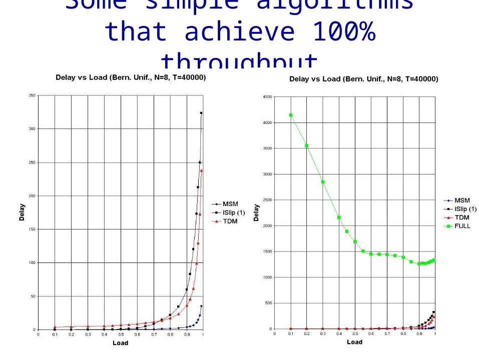
Some simple algorithms that achieve 100% throughput

31
Some observations
A maximum size match (MSM) maximizes instantaneous throughput.
But a MSM is complex – O(N2.5). It turns out that there are many simple
algorithms that give 100% throughput for uniform traffic.
So what happens if the traffic is non-uniform?

32
Why doesn’t maximizing instantaneous throughput give 100% throughput for non-
uniform traffic?
2/1
2/1
2/1
32
21
1211Three possiblematches, S(n):
100%). t(throughpu stable not is switch 0.0358 if so And
But
most at is served is 1 input which at rate total The
. w.p. serviced is 1 Input ) w.p.( arrivals have
both and and , time at that Assume
.)21(31121
.)21(311
)21(11)21(32
32)21(
)()(0)(0)(
21
2
22
2
32211211
-δ// - -λ
//
/-//
/-δ/
nQnQ n, L nn, L
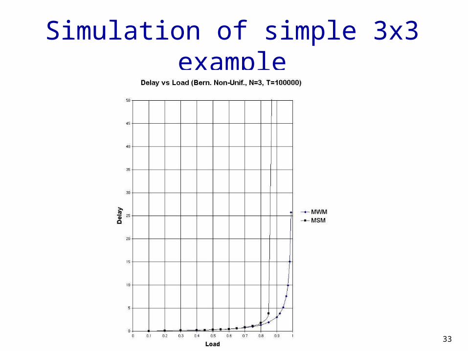
33
Simulation of simple 3x3 example

34
Scheduling algorithms to achieve 100% throughput
1. Basic switch model.2. When traffic is uniform (Many algorithms…)3. When traffic is non-uniform, but traffic matrix is known
• Technique: Birkhoff-von Neumann decomposition.
4. When matrix is not known.• Technique: Lyapunov function.
5. When algorithm is pipelined, or information is incomplete.• Technique: Lyapunov function.
6. When algorithm does not complete.• Technique: Randomized algorithm.
7. When there is speedup.• Technique: Fluid model.
8. When there is no algorithm.• Technique: 2-stage load-balancing switch.• Technique: Parallel Packet Switch.

35
Example 1: (Trivial) scheduling to achieve 100%
throughput
Assume we know the traffic matrix, and the arrival pattern is deterministic:
Then we can simply choose:
1000
0100
0010
0001
nnS
,
10
...
1
01
)(

36
Example 2:With random arrivals, but known traffic
matrix Assume we know the traffic matrix, and the arrival pattern is random:
Then we can simply choose:
In general, if we know , can we pick a sequence S(n) to achieve 100% throughput?
1000
0100
002/12/1
002/12/1
1000
0100
0001
0010
)(,
1000
0100
0010
0001
)( evenSoddS

37
Birkhoff - von Neumann Decomposition
rate. arrival the exceeds rate
departure the and words, other In
is period in of soccurrence of# the that So
:matrices service of sequence the pick Then
element) by (element
:that such matrices, service of set and
constants of set some pick can we y,Intuitivel
,0))((
.
),,,,,,,()(
.,
),(
),,(
1
13221
1
1
1
T
i
ii
r
r
iii
r
r
iS
aTM
T
MMMMMMnS
Ma
MM
aa
Any can be decomposed into a linear (convex) combination of matrices, (M1, …, Mr).
38
In practice…
Unfortunately, we usually don’t know traffic matrix a priori, so we can: Measure or estimate , or Not use .
In what follows, we will assume we don’t know or use .

39
Scheduling algorithms to achieve 100% throughput
1. Basic switch model.2. When traffic is uniform (Many algorithms…)3. When traffic is non-uniform, but traffic matrix is known
• Technique: Birkhoff-von Neumann decomposition.
4. When traffic matrix is not known.• Technique: Lyapunov function.
5. When algorithm is pipelined, or information is incomplete.• Technique: Lyapunov function.
6. When algorithm does not complete.• Technique: Randomized algorithm.
7. When there is speedup.• Technique: Fluid model.
8. When there is no algorithm.• Technique: 2-stage load-balancing switch.• Technique: Parallel Packet Switch.

40
When the traffic matrix is not known
( 1) ( ) ( ) 0
( ) ( ) ( ) ( ) | ( ) 0.
( 1) ( ) ( ) ( ) .
1. We will try and fi nd conditions f or which:
i.e.
2. Usually we can only fi nd,
ij ij
ij ijij ij
E V L n V L n | L n ,
E V L n S n A n V L n L n
E V L n V L n | L n c k L n

41
Problem
1 1
( )
( )
max ( ( ) )
1 1 0.
'
max( ( ) ) max( ( ) ( )).
( ( ) ) max( ( ) ( )) 0.
Find:
s.t.
We know that the solution is an
extreme point of the set of all .
i.e.
What is
T
N N
ij ij iji j
T T
λ S n
T T
S n
L n
λ , λ , λ
s
L n λ L n S n
L n λ L n S n
( )max( ( ) ( ))? T
S nL n S n

42
Maximum weight matching
A1(n)
N NLNN(n)
A1N(n)
A11(n)
L11(n)
1 1
AN(n)
ANN(n)
AN1(n)
D1(n)
DN(n)
L11(n)
LN1(n)
“Request” Graph Bipartite Match
S*(n)
MaximumWeight Match
*
( )( ) arg max( ( ) ( ))T
S nS n L n S n

43
Outline of Proof*
( )
*
( ) arg max( ( ) ( )),
( ( ) ) ( ( ) ( )) 0.
( 1) ( 1) ( ) ( ) ( ) ( ) .
{ ( )} ( ) ( ),
1. Pick
then
2. I t f ollows that:
where: is our Lyapunov f unction.
3. Hence, i
T
S n
T T
T T
T
S n L n S n
L n λ L n S n
E L n L n L n L n | L n c L n
V L n L n L n
( )
[ ( )]
f is large enough, there is an expected
single-step downward drif t in occupancy, and so
.
L n
E L n

44
Choosing the weight
2 3
( ) ( )?
( ) [ ( )] ,[ ( )] ,...
[ ( )]
( ) [ ( )] [ ( )] .
Q: Do we need to choose edge weights:
I f we choose then same
Lyapunov method gives .
I f then For ex
ij ij
ij ij ij
ij
xxij ij ij
w n L n
w n L n L n
E L n
w n L n E L n
Fact 1:
Fact 2:
( ) ( ) [ ( )] .
( )
ample,
if , then
Simulation suggests that average delay decreases as we increase .
I f is defi ned to be the time that the HOL cell
has been in queue
ij ij ij
ij
w n L n E L n
x
w n
Observation:
Fact 3:
[ ( )]
( ) ( ) ( ) [ ( )] .
, then .
I f , then
This is called a "Longest Port First (LPF)" match, and
(surprisingly) is also a maximum size match.
ij ij
ij ij ij iji j
Q E L n
w n L n L n E L n
Fact 4:
45
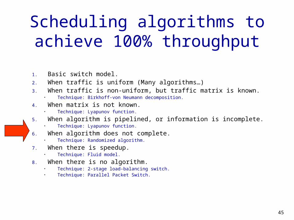
Scheduling algorithms to achieve 100% throughput
1. Basic switch model.2. When traffic is uniform (Many algorithms…)3. When traffic is non-uniform, but traffic matrix is known.
• Technique: Birkhoff-von Neumann decomposition.
4. When matrix is not known.• Technique: Lyapunov function.
5. When algorithm is pipelined, or information is incomplete.• Technique: Lyapunov function.
6. When algorithm does not complete.• Technique: Randomized algorithm.
7. When there is speedup.• Technique: Fluid model.
8. When there is no algorithm.• Technique: 2-stage load-balancing switch.• Technique: Parallel Packet Switch.
46
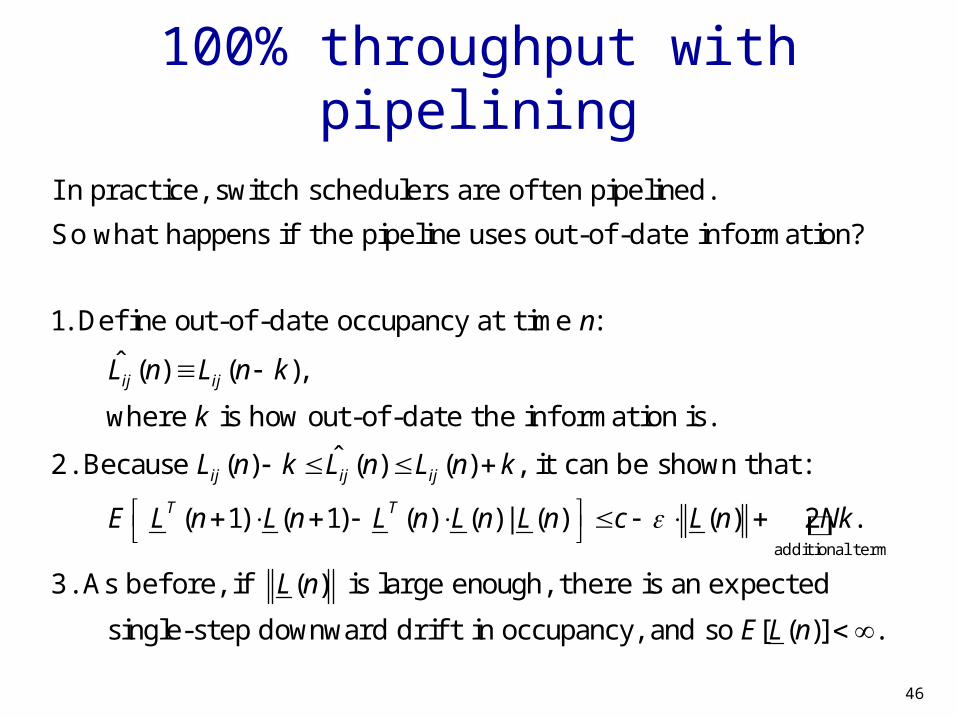
100% throughput with pipelining
ˆ ( ) ( ),
I n practice, switch schedulers are of ten pipelined.
So what happens if the pipeline uses out-of -date inf ormation?
1. Defi ne out-of -date occupancy at time :
where is how out-of -date thij ij
n
L n L n k
k
ˆ( ) ( ) ( ) ,
( 1) ( 1) ( ) ( ) ( ) ( ) 2 .
( )additional term
e inf ormation is.
2. Because it can be shown that:
3. As bef ore, if is large enough, there is an expecte
ij ij ij
T T
L n k L n L n k
E L n L n L n L n | L n c L n Nk
L n
[ ( )]
d
single-step downward drif t in occupancy, and so .E L n

47
100% throughput with incomplete information
I n practice, the bandwidth of state inf ormation to/ f rom
and within a switch schedulers is limited.
So what happens if the scheduler uses f ewer bits to store
the weight inf ormation?
1. Defi ne noisy inf orma
ˆ( ) ( ) ( ),
( )
( ) [ ( )] .
tion at time :
where is an error term.
2. I f , , where is some constant, then ij
n
L n L n e n
e n
e n C n C E L n

48
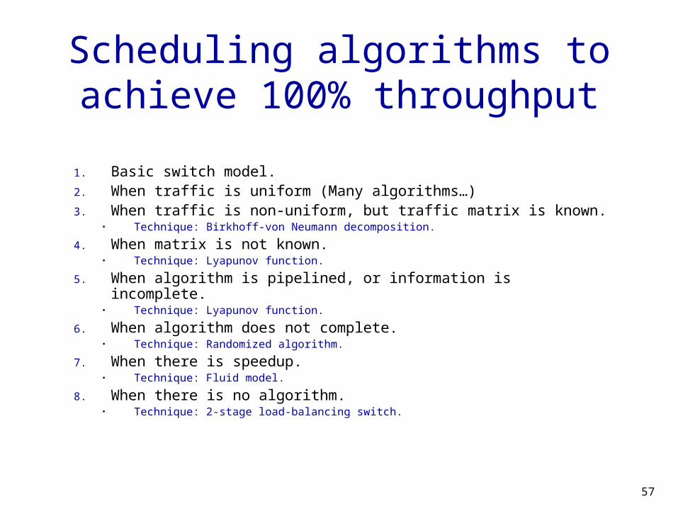
Scheduling algorithms to achieve 100% throughput
1. Basic switch model.2. When traffic is uniform (Many algorithms…)3. When traffic is non-uniform, but traffic matrix is known.
• Technique: Birkhoff-von Neumann decomposition.
4. When matrix is not known.• Technique: Lyapunov function.
5. When algorithm is pipelined, or information is incomplete.• Technique: Lyapunov function.
6. When algorithm does not complete.• Technique: Randomized algorithm.
7. When there is speedup.• Technique: Fluid model.
8. When there is no algorithm.• Technique: 2-stage load-balancing switch.• Technique: Parallel Packet Switch.
49
Achieving 100% when algorithm does not complete
Randomized algorithms:1. Basic idea (Tassiulas)2. Reducing delay (Shah, Giaccone and Prabhakar)

50
Scheduling algorithms to achieve 100% throughput
1. Basic switch model.2. When traffic is uniform (Many algorithms…)3. When traffic is non-uniform, but traffic matrix is known.
• Technique: Birkhoff-von Neumann decomposition.
4. When matrix is not known.• Technique: Lyapunov function.
5. When algorithm is pipelined, or information is incomplete.• Technique: Lyapunov function.
6. When algorithm does not complete.• Technique: Randomized algorithm.
7. When there is speedup.• Technique: Fluid model.
8. When there is no algorithm.• Technique: 2-stage load-balancing switch.• Technique: Parallel Packet Switch.

51
Speedup and Combined Input Output Queueing (CIOQ)
A1(n)
S(n)
N NLNN(n)
A1N(n)
A11(n)L11(n)
1 1
AN(n)
ANN(n)
AN1(n)
D1(n)
DN(n)
With speedup, the matching is performed s times per cell time, and up to s cells are removed from each VOQ. Therefore, output queues are required.

52
Fluid Model [Dai and Prabhakar]
{ ( ) 0)1
( ) (0) ( ) ( )
( ) 1 ( ( ) ( 1)),
( )
( ) .
Switch evolution:
where: is the cumulative time permutation
has been used by slot ; and
Fluid equations
ij
ij ij ij ij
nm m
ij ij L k s ss S k
mS
ms
s S
L n L A n D n
D n s T k T k
T n S
n T n n
( ) (0) ( )
( ) ( ), ( ) .
( )( )lim lim
in continuous time:
where:
Result:
ij ij ij ij
m mij ij s s
s S s S
ijijij
n n
L t L t D t
D t s T t T t t
A nD n
n n

53
Scheduling algorithms to achieve 100% throughput
1. Basic switch model.2. When traffic is uniform (Many algorithms…)3. When traffic is non-uniform, but traffic matrix is known.
• Technique: Birkhoff-von Neumann decomposition.
4. When matrix is not known.• Technique: Lyapunov function.
5. When algorithm is pipelined, or information is incomplete.• Technique: Lyapunov function.
6. When algorithm does not complete.• Technique: Randomized algorithm.
7. When there is speedup.• Technique: Fluid model.
8. When there is no algorithm.• Technique: 2-stage load-balancing switch.

54
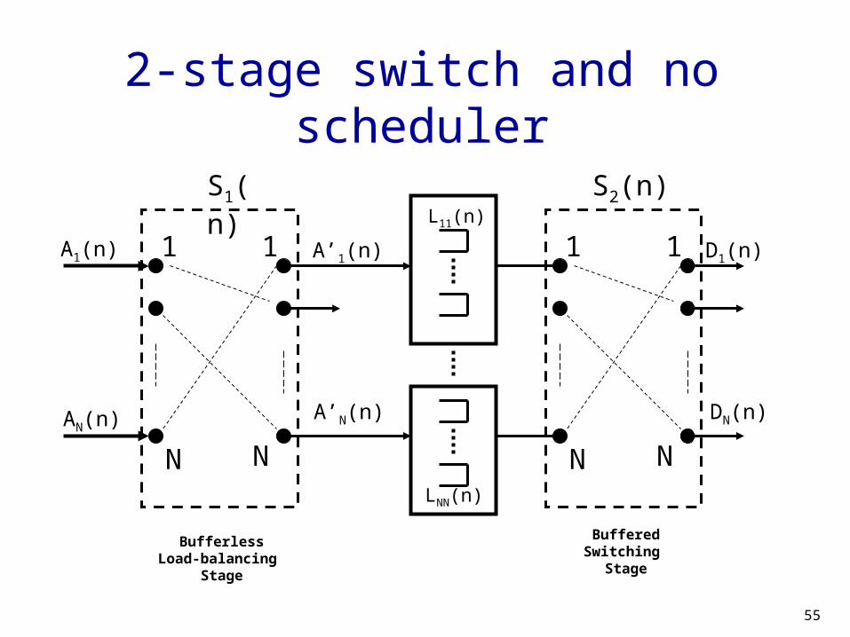
2-stage switch and no scheduler
Motivation:1. If traffic is uniformly distributed, then
even a deterministic schedule gives 100% throughput.
2. So why not force non-uniform traffic to be uniformly distributed?
55
2-stage switch and no scheduler
S2(n)
N NLNN(n)
L11(n)
1 1 D1(n)
DN(n)
N N
1 1 A’1(n)
A’N(n)
S1(n)
A1(n)
AN(n)
BufferlessLoad-balancing
Stage
BufferedSwitching
Stage

56
2-stage switch with no scheduler
ˆ( ) ,
ˆ mod
1. Consider a periodic sequence of permutation matrices:
where is a one-cycle permutation matrix
and .
2. I f 1st stage is scheduled by a sequence of per
nn
n n N
Main Result [Chang et al.]:
1 1
1
2 2
( ) ( ),
( ) ( ),
mutation
matrices:
where is a random phase, and
3. The 2nd stage is scheduled by a sequence of permutation
matrices:
4. Then the switch gives 100% throughput f or weakly mix
n n
n n
ing arrivals.
1st stage makes non-unif orm traffi c unif orm,
and breaks up burstiness. For bursty traffi c, delay can be
lower than f or an output queued switch.
Cells can become m
Observation 1:
Observation 2: is-sequenced.
57
Scheduling algorithms to achieve 100% throughput
1. Basic switch model.2. When traffic is uniform (Many algorithms…)3. When traffic is non-uniform, but traffic matrix is known.
• Technique: Birkhoff-von Neumann decomposition.
4. When matrix is not known.• Technique: Lyapunov function.
5. When algorithm is pipelined, or information is incomplete.• Technique: Lyapunov function.
6. When algorithm does not complete.• Technique: Randomized algorithm.
7. When there is speedup.• Technique: Fluid model.
8. When there is no algorithm.• Technique: 2-stage load-balancing switch.

58
Throughput resultsTheory:
Practice:
InputQueueing
(IQ)
InputQueueing
(IQ)
InputQueueing
(IQ)
InputQueueing
(IQ)
58% [Karol, 1987]
IQ + VOQ,Maximum weight matching
IQ + VOQ,Maximum weight matching
IQ + VOQ,Sub-maximal size matching
e.g. PIM, iSLIP.
IQ + VOQ,Sub-maximal size matching
e.g. PIM, iSLIP.
100% [M et al., 1995]
Different weight functions,incomplete information, pipelining.
Different weight functions,incomplete information, pipelining.
Randomized algorithmsRandomized algorithms
100% [Tassiulas, 1998]
100% [Various]
Various heuristics, distributed algorithms,
and amounts of speedup
Various heuristics, distributed algorithms,
and amounts of speedup
IQ + VOQ,Maximal size matching,
Speedup of two.
IQ + VOQ,Maximal size matching,
Speedup of two.
100% [Dai & Prabhakar, 2000]
59
Outline of next talkSundar Iyer
What’s known about controllable delay Emulation of Output queued switches PIFOs and WFQ Single-buffered switches: Parallel packet switches,
and distributed shared memory switches.