1

Image and Video Compression

Wenwu Wang

Centre for Vision Speech and Signal Processing

Department of Electronic Engineering

University of Surrey

Email: w.wang@surrey.ac.uk

2

Introduction

• Course components

• A brief history

• Basic concepts

• Coding performance limits

• Coding of still image

3

Course Components

• Component Coding Algorithms I (By myself) Fundamentals of Compression Coding of Still image JPEG standard Vector Quantisation Subband and Wavelet Coding

• Component Coding Algorithms II (By Dr Fernando) Coding of video sequence, H.261, 263, coding algorithms MPEG-1, -2, -4 coding algorithms

• Component Error Resilience in Video Communications (By Prof. Kondoz)

4

Further Reading• Component Coding Algorithms

• Ghanbari, M. Standard Codecs: Image Compression to Advanced Video Coding, IEE Telecommunication Series 49, 2003. 0-85296-710-1 A

• Clarke, R. J. Digital Compression of Still Images and Video, Academic Press, 1995. 0-12-175720-X B

• Haskell, B. G., Puri, A. and Netravali, A. N. Digital Video: An Introduction to MPEG-2, Chapman and Hall, 1997. 0-412-08411-2 B

Error Resilience

• Sadka, A. H. Compressed Video Communications, J. Wiley and Co, 2001. 0-470843128 A More References

5

A Brief History of Image Communication• 1840 Louis J.M. Daguerre, France,

William Henry Fox Talbot, USA, photographic film• 1895 First public motion picture presentation• 1920s First television experiment

British TV pioneer J.L. Baird with Nipkow Disc (around 1926)

6

A Brief History of Image Comm. (Cont)

• 1930s Color movies• 1930-32 First experimental television broadcasting in US• 1935 First German television broadcasting in Berlin• 1936 TV transmission during the Berlin Olympics

British TV pioneer J.L. Baird with Nipkow Disc (around 1926)

7

A Brief History of Image Comm. (Cont.)• 1939 Regular monochrome TV service in US• 1952 Regular TV service in Germany• 1954 NTSC Color television in US• 1967 PAL color television in Germany• 1970s Consumer video cassette recorder (VCR)• 1970s Fax machines• 1980s Digital TV studios (ITU-R rec. 601)

8

A Brief History of Image Comm. (Cont.)

• 1990s JPEG and MPEG standards

Digital still cameras

Digital TV broadcasting

Digital video/versatile disk (DVD)

Integration of computers and video

World wide web

Internet video streaming

9

A Brief History of Image Comm. (Cont.)

Evolution of the video coding standard by the ITU-T and ISO/IEC committees

10

Fundamentals

11

What?

• The minimisation of the amount of information required to represent an image/video signal

• The reduction of the overall signal bandwidth

12

Why?

• Applications for which bandwidth is a precious commodity

• Storage applications:

Archiving, television production, home entertainment, multimedia

• Transmission applications:

Radio and television broadcasting, internet video streaming, multimedia for mobile phones

13

How?• Image and video signals contain superfluous (redundant) information

• Statistical redundancy associated with signal predictability/correlation/smoothness:

Original signal can be recovered perfectly, therefore it is called “lossless” or “information preserving” coding

• Subjective redundancy associated with the error tolerance of human vision:

Original signal cannot be recovered perfectly, only an approximate reconstruction is possible, therefore it is called “lossy” or “error tolerant” coding

14

Performance Assessment

• Efficiency in image and video coding(an indication of how much information has been reduced for the coded

signal) lossless systems: ratios of uncoded-to-coded

information, i.e. compression ratio lossy systems: the amount of coded information

expressed as a function of the distortion introduced by the coding operation, i.e. rate/distortion function

• Distortion in image and video coding(an indication of how close to the original is the coded signal) lossless systems: trivially zero distortion (infinite fidelity) lossy systems: distortion can be measured objectively

(computation of error between the original and the coded representation) or subjectively (tests designed to measure response of human vision to coding artefacts)

15

Coding Operation in the Image Chain• Signal processing operations anywhere in the image chain

can be regarded as coding operations. Such operations may be due to:

Acquisition environment (such as lighting conditions and light propagation, special effects in studio, and atmospheric conditions in outside broadcasts)

Acquisition systems (such as camera optics, scanning aperture and field integration in electronic imaging, and chemical process in film)

Post-production environment (such as special effects) Image/video display systems (such as display aperture in electronic

imaging, half-toning in printed media, and chemical process in film) Viewing environment (such as propagation of light, and optical paths) Human visual system (such as lens, and response of neurons to light

stimuli)• We are not concerned with the above but need to be aware of their

coding effects.• We are concerned with the processing of image/video signals after

acquisition/post-production and prior to display

16

Classification of Video Coding Sytems• Analogue (signals predominantly in analogue form) PAL (Phase Alternating Line, transmission of terrestrial television) VHS (Video Home System, home video recording) MAC (Multiplexed Analogue Component, satellite television transmission) Betacam SP (Superior Performance, video recording in the studio)

• Digital (signals predominantly in digital form) ITU-R Rec. 601 (BT.601, or CCIR-601) (professional video recording) MPEG-1 (home video recording, CD-ROM) MPEG-2 (television transmission) MPEG-4 (multimedia) H.261/3 (video conferencing) JPEG (still images)

• We will be mainly concerned with digital signals in this module. For more about analogue signals, please refer to some textbooks. Here, we only introduce a few fundamentals about analogue signals that closely related to digital signals.

17

Coding of Colour Signals

• One of the challenges facing the first of colour television systems was the inclusion of colour information without increasing the video bandwidth.

• Colour cameras operate in the space of R,G,B primaries. Each of these component signals are full-bandwidth (i.e. 6.75MHz)

• Colour coding systems (i.e. PAL) typically involve the conversion of component signals to composite by means of the following processing operations:

R,G,B to Y,U,V co-ordinate transformation Low-pass filtering of U and V components DSSC-AM modulation of U and V by two sub-carriers in phase

quadrature Sign alternation of modulated V at every other line

18

Coding of Colour Signals (Cont.)

587.0,114.0,299.0,

)1/()(615.0

)1/()(436.0

GBR

R

B

BGR

WWWwhere

WYRV

WYBU

BWGWRWY

19

Coding of Colour Signals (Cont.)• Y – Luma component, representing the brightness of

an image (i.e. the “black and white” or achromatic portion of the image).

• U – Blue difference chroma (B-Y)• V – Red difference chroma (R-Y)• “Luma” and “chroma” are usually used in video

engineering, while “luminance” and “chrominance” are used in color science.

• In digital domain, YCbCr is used to represent the coded color, where DSSC-AM modulation is replaced by subsampling.

20

Consequence of Colour Coding• Compression ration: 3:1• Artefacts Visible line structure, and interline flicker, Combing (distortion of vertical detail moving horizontally due to interlace) Spatial aliasing (i.e. diagonal straight lines cause spatial “beat” frequencies

and jagged/staircase edges) Temporal aliasing (fast motion suffers from “judder”) Picture “softness” (aperture effects)

• Artefact frequency: low• Artefact severity: high• Remedies At the transmitter end, intelligent PAL encoding allowing better segregation

of colour and monochrome components with less crosstalk between them At the receiver end, intelligent PAL decoding possibly involving motion

adaptive filtering (may attenuate some frequency components)

21

Digital Video Formats – A Case Study of Digital Television

• This format is standardised and is described in the document “Recommendation ITU-R BT.601”.

• Source signals: Y,U,V (one luminance and two colour-difference components, gamma pre-corrected and filtered)

• Sampling structure (625 line/50Hz analogue system) Orthogonal, line, field and frame repetitive U,V samples co-sited with odd Y samples in each line 864 total (720 active) luminance samples per line 432 total (360 active) chrominance samples per line 625 total (576 active) lines

• Sampling frequency (Y:135MHz, U,V:6.75MHz)• Quantisation Uniformly quantised PCM 8 (optionally 10) bits per sample Scale 0-255 Luminance black level defined as level 16 Luminance peak white level defined as level 235 Luminance total number of active levels 220 Chrominance total number of active levels 225 with zero corresponding to 128

22

Digital Video Formats – A Case Study of Digital Television (Cont.)

• Total active bit-rate 720 samples/line X 576 lines/frame X 25 frames/sec X 8

bits/sample/component X (1+0.5+0.5) components = 166 Mbits/sec

• Total raw bit-rate (Y:135MHz, U,V:6.75MHz) 864 samples/line X 625 lines/frame X 25 frames/sec X 8

bits/sample/component X (1+0.5+0.5) components = 216 Mbits/sec

For television transmission purposes this amount of information may require (depending on the modulation scheme) a bandwidth of 40 MHz upwards

Today this corresponds to occupancy requirements of 6-7 analogue terrestrial television channels !! Therefore, to make digital television transmission a practical proposition compression in the digital domain is imperative.

23

Digital Video Formats – A Case Study of Digital Television (Cont.)

• Note 1 Unused samples and levels are actually used to convey auxiliary and

control information i.e. vertical and horizontal synchronisation (blanking), colour reference (burst) etc. There are applications which require this information in digital form

• Note 2 The 601 standard is a specification of the output format only and is

not concerned with the practical implementation of the A/D conversion. This is left to the system designer to implement but should typically involve anti-aliasing pre-filtering and attention to the effects of the non-ideal sampling aperture and pixel aspect ratio.

24

Digital Video Formats – Other Formats

• High-definition television (HDTV) 1920 X 1152 X 50 Hz interlaced (16:9 aspect ratio) 1440 X 1152 X 50 Hz interlaced (4:3 aspect ratio)

• Video-conferencing/Video-telephony 352 X 288 X 30 Hz Progressive CIF (Common Interchange Format) 352 X 288 (240) X 25 (30) Hz progressive SIF (Source Input Format-PAL

(NTSC)) 176 X 144 X 30 Hz Progressive QCIF (Quarter CIF)

• Composite (PAL) digital video (recording) 922 X 576 X 50 Hz interlaced This results from sampling a composite (PAL) signal with a frequency which

is 4 times the colour subcarrier frequency and is used for the recording of digital composite signals for studio applications

• Desktop 800 X 600 Super VGA (Vector Graphic Array) 640 X 480 VGA

25

The Hierarchy of Video Sampling Format

26

Sampling Formats for Chrominance

27

Coding Performance Limits and Assessment

28

Self-Information

• A discrete source with a finite alphabet A can be modelled as a discrete random process i.e. a sequence of random variables

• Each random variable takes a value from the alphabet

• The information content of a symbol is related to the degree that the symbol is unpredictable and unexpected. Quantitatively this can be expressed by means of the self-information of symbol

(bits)

X

,...}2,1|{ kaA k

ix,...2,1, ixi

ka

ka)( kaI

))((log)( 2 kk apaI

29

Source Models

• Two useful source models are used for the studying the coding performance limit:

The Discrete Memoryless Source (DMS) Successive symbols are statistically independent i.e. in a symbol

sequence the current symbol does not depend on any previous one

The Markov K-th order Source (MKS) Successive symbols are statistically dependent i.e. in a symbol

sequence the current symbol depends on the K previous ones

The entropy of a DMS source X is defined as the average self-information:

The entropy is maximised for a uniform symbol distribution.

k

kkk

kk aapaIapXH )(log)()()()( 2

30

Markov-K Source

• The MKS model is a more realistic model for images and video Images (of natural scenes) are correlated in the spatial domain i.e. plain

areas (with little or no spatial detail) Video is correlated in the spatial domain as above and also in the temporal

domain i.e. static areas (with little or no motion)

• A MKS can be specified by the following conditional probabilities:

• The entropy of a MKS source is defined as

kiXXaXp kiiki ,),...,|( 1

kiXXXHXXaXpXHkS

kiikiiki ,),...,|(),...,|()( 11

where is the conditional entropy i.e. ),...,|( 1 kii XXXH

i

kiikikiiki XXaXpXXaXp )),...,|((log),...,|( 121

and denotes all possible realisations kS },...,{ 1 kii XX

31

Coding Theorem

32

Coding Theorem (cont.)

A typical rate distortion curve

33

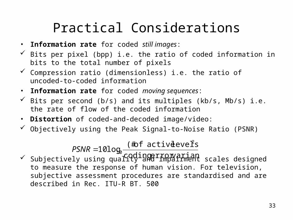
Practical Considerations• Information rate for coded still images: Bits per pixel (bpp) i.e. the ratio of coded information in bits to the total

number of pixels Compression ratio (dimensionless) i.e. the ratio of uncoded-to-coded

information

• Information rate for coded moving sequences: Bits per second (b/s) and its multiples (kb/s, Mb/s) i.e. the rate of flow of the

coded information

• Distortion of coded-and-decoded image/video: Objectively using the Peak Signal-to-Noise Ratio (PSNR)

Subjectively using quality and impairment scales designed to measure the response of human vision. For television, subjective assessment procedures are standardised and are described in Rec. ITU-R BT. 500

varianceerrorcoding

levels)activeof(#log10

2

10PSNR

34

Subjective Picture Assessment for Television

35

Human Visual System

Plot of contrast sensitivity (just perceptual modulation) function

36

Human Visual System (Cont.)

37

Coding of Still Images

38

Classification of Compression Techniques

• Spatial (data) Domain Elements are used “raw” in suitable combinations. The

frequency of occurrence of such combinations is used to influence the design of the coder so that shorter codewords are used for more frequent combinations and vice versa (entropy coding).

• Transform Domain Elements are mapped onto a different domain (i.e. the

frequency domain). The resulting coefficients are quantised and entropy-coded.

• Hybrid Combinations of the above.

39

Lossless Coding in the Spatial Domain

• Memoryless Coding

40

Lossless Coding in the Spatial Domain (Cont.)

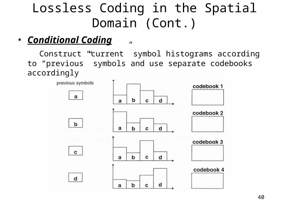
• Conditional Coding

Construct “current” symbol histograms according to “previous” symbols and use separate codebooks accordingly

41

Lossless Coding in the Spatial Domain (Cont.)• Block (joint) Coding Define blocks of more than one symbols and record their occurrences using a

multi-dimensional histogram Code book grows exponentially with block size Useful when symbols in a block are correlated

An example using a block size of 2 i.e. two consecutive symbols.

42

Lossless Coding in the Spatial Domain (Cont.)

• Predictive Coding (previous symbol) “Previous” symbol used as a prediction of “current” symbol Prediction error coded in a memoryless fashion Prediction error alphabet and codebook have twice the size

i.e. symbol alphabet {1, 2, 3, 4} prediction alphabet {-3, -2, -1, 0, 1, 2, 3} A good predictor will minimise the error (most occurrence will be zero)

43

Lossless Coding in the Spatial Domain (Cont.)

• Predictive Coding (generalised) Prediction is based on combination of

previous symbols Prediction template needs to be “causal” i.e.

template should contain only “previous” elements w.r.t the direction of scanning (shown with arrows). This is important for coding applications as the decoder will need to have decoded the template elements first to perform the prediction of the current element.

44

Lossless Coding in the Spatial Domain (Cont.)

• Run-length Coding Useful when consecutive symbols in a string are identical A symbol is followed by the number of its repetitions

A typical example

A general example

45

Lossless Coding in the Spatial Domain (Cont.)• Zero Run-length Coding Useful for strings containing long runs of consecutive zeros and are

sparsely populated by non-zero symbols i.e. quantised frame differences

A non-zero symbol is followed by the number of consecutive zeros

A typical example

A general example

46

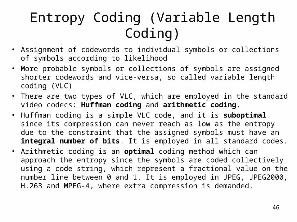
Entropy Coding (Variable Length Coding)

• Assignment of codewords to individual symbols or collections of symbols according to likelihood

• More probable symbols or collections of symbols are assigned shorter codewords and vice-versa, so called variable length coding (VLC)

• There are two types of VLC, which are employed in the standard video codecs: Huffman coding and arithmetic coding.

• Huffman coding is a simple VLC code, and it is suboptimal since its compression can never reach as low as the entropy due to the constraint that the assigned symbols must have an integral number of bits. It is employed in all standard codes.

• Arithmetic coding is an optimal coding method which can approach the entropy since the symbols are coded collectively using a code string, which represent a fractional value on the number line between 0 and 1. It is employed in JPEG, JPEG2000, H.263 and MPEG-4, where extra compression is demanded.

47

Huffman Coding

48

Huffman Coding (Cont.)

An example of Huffman code for seven symbols

Entropy:

Average bit per symbol:

49

Arithmetic Coding

• Using a scale in which the coding intervals of real numbers between 0 and 1 are represented. This is in fact the cumulative probability density function of all the symbols which add up to 1.

• The interval is partitioned according to symbol likelihood.• The interval is iteratively reduced by retaining, at each

iteration, the sub-interval corresponding to the currently encoded input symbol

50

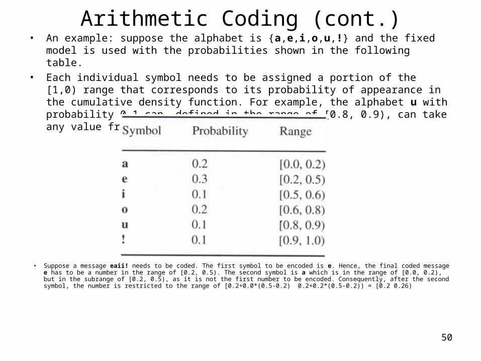
Arithmetic Coding (cont.)• An example: suppose the alphabet is {a,e,i,o,u,!} and the fixed model is used with the

probabilities shown in the following table.• Each individual symbol needs to be assigned a portion of the [1,0) range that

corresponds to its probability of appearance in the cumulative density function. For example, the alphabet u with probability 0.1 can, defined in the range of [0.8, 0.9), can take any value from 0.8 to 0.89999…

• Suppose a message eaii! needs to be coded. The first symbol to be encoded is e. Hence, the final coded message e has to be a number in the range of [0.2, 0.5). The second symbol is a which is in the range of [0.0, 0.2), but in the subrange of [0.2, 0.5), as it is not the first number to be encoded. Consequently, after the second symbol, the number is restricted to the range of [0.2+0.0*(0.5-0.2) 0.2+0.2*(0.5-0.2)) = [0.2 0.26)

51

Arithmetic Coding (cont.)• The next symbol to be encoded is I, in the range of [0.5, 0.6), that corresponds to the

new subrange [0.2, 0.26). Hence, after this symbol, the coded number is restricted to the range of [0.2+0.5*(0.26-0.2), 0.2+0.6*(0.26-0.2)) = [0.23, 0.236). Applying the same rule to the successive symbols. We can obtain the following table:

• The final range [0.23354, 0.2336) represents the message eaii!. This means if we transmit any number in the range of [0.23354, 0.2336), that number represents the whole message of eaii!.

52

Arithmetic Coding (cont.)

Representation of arithmetic coding process with the interval scaled up at each stage for the message eaii!

53

Arithmetic Coding (cont.)• Decoding process For the previous example, suppose a number 0.23355 in the range of [0.23354,

0.2336) is transmitted. The decoder, using the same probability intervals as the encoder, performs a similar procedure.

Only the interval [0.2, 0.5) of e envelops the transmitted code of 0.23355. So the first symbol can only be e. The new code for the second symbol is (0.23355-0.2)/(0.5-0.2)=0.11185, which is enveloped by interval [0.0, 0.2) of symbol a. The new code for the third symbol is (0.11185-0.0)/(0.2-0.0) = 0.55925, which is enveloped by the range of [0.5, 0.6) of symbol i. Followed by (0.55925-0.5)/(0.6-0.5) = 0.5925 in the range of [0.5, 0.6) of symbol i. Further followed (0.5925-0.5)/(0.6-0.5) = 0.925, which is in the range of [0.9, 1) of symbol !. Therefore, the decoded message is eaii!. The decoding process is shown in the following table:

54

Lossless Coding in Transform Domain

• Transforms commonly refer to expansions of signals to series of coefficients using sets of appropriate (i.e. orthonormal) basis functions so that the following are achieved.

Decorrelation of input data Optimal distribution of energy (variance) into the smallest number

of coefficients

• The optimal transform according to the above is the Karhunen-Loeve (KL) transform. This is not used in practice:

Its basis functions are the eigenvectors of the covariance matrix of the input signal, and hence data-dependent, and therefore need to be computed and transmitted for each data set.

There are no fast implementations for the KL transform

55

Lossless Coding in Transform Domain (cont.)

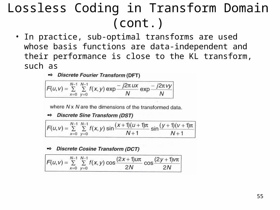
• In practice, sub-optimal transforms are used whose basis functions are data-independent and their performance is close to the KL transform, such as

56

Lossless Coding in Transform Domain (cont.)• The DCT is the most widely used transform in image/video coding and is a

fundamental component of many standardised algorithms. KLT and DCT basis functions closely resemble each other for images modelled as

first-order Markov processes. A n-point DCT is equivalent to a 2n-point DFT obtained by reflection. This avoids

spurious harmonics due to discontinuities at the boundaries of the repetition period.

• The following example visualises the decorrelation and energy compaction properties of transforms:

57

Lossless Coding in Transform Domain (cont.)

58

Comparison of Various Transforms

59

Comparison of Various Transforms (cont.)

(1) Energy concentration measured typical natural images of block size 1-by-32.

(2) KLT is optimum and DCT performs slightly worse than KLT

60

Block Transform Coding

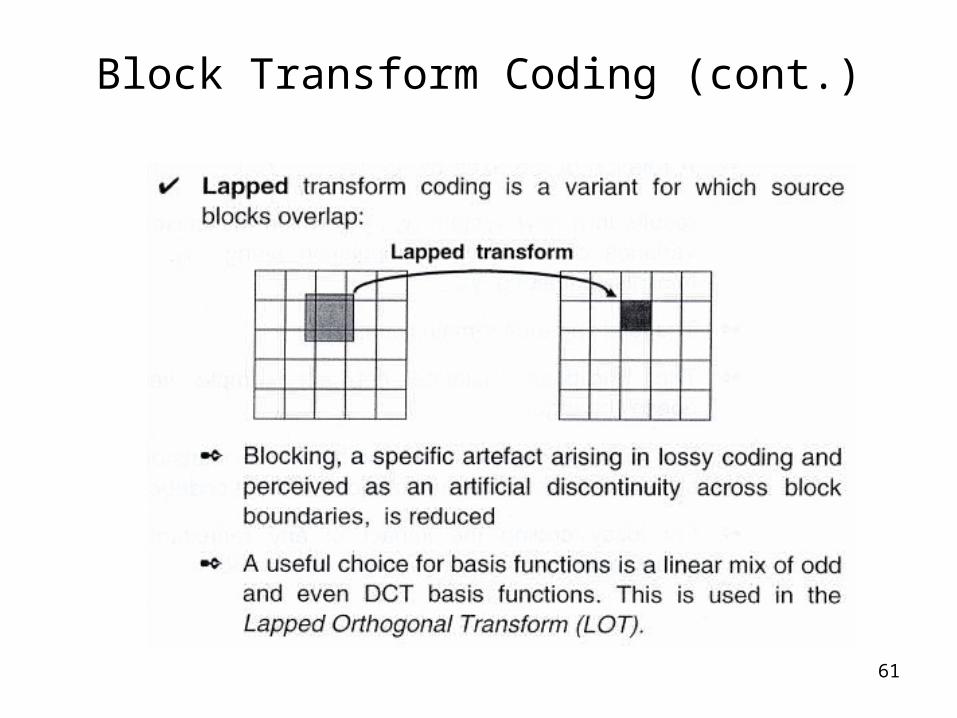
61

Block Transform Coding (cont.)

62

Block Transform Coding (cont.)

63

Lossy Coding

• For natural images the compression performacne of lossless coding schemes is fairly modest

Compression ratios of 3:1 or 4:1 can be achieved using the best of the above mentioned schemes.

This is comparable to the performance achieved by the general purpose data compression algorithms i.e. Ziv-Lempel, which are not designed specifically to exploit image structure.

• To improve performance some coding distortion will have to be tolerated. The main aims of lossy coding are:

To optimise rate/distortion performance i.e. achieve the best image quality for a given target bit-rate

To minimise the perceptual impact of distortion i.e. produce coding errors that are likely to be imperceptible to the human viewer

64

Lossy Coding (cont.)

• The main tool for lossy coding is quantisation. This is applicable to most domains:

Spatial (data) domain: applicable to raw pixels, pixel differences (predictive coding), conditional pixel occurrences (conditional coding), ensembles of pixels (joint coding). This is a special case of so-called vector quantisation which will be studied separately.

Transform domain: applicable to transform coefficients and ensembles of coefficients (vector quantisation).

• Another important tool is sampling This is usually applicable to the data domain.

65

Quantisation (scalar)

66

Lossy Predictive Coding

Open-loop encoder (prediction based on past inputs)

Closed-loop encoder (prediction based on past outputs)

Decoder (prediction always based on past outputs)

67

Lossy Transform Coding

Coder

Decoder

68

Sampling: One-dimensional sampling

69

Sampling: One-dimensional sampling (cont.)

70

Sampling: Two-dimensional sampling

71

Sampling: Two-dimensional sampling (cont.)

72

Sampling: Two-dimensional sampling (cont.)

73

Non-ideal Sampling

74

Interpolation

75

Non-ideal Interpolation (sample-and-hold)

76

Non-ideal Interpolation (bi-linear)

77

Example of Non-ideal Interpolation

78

Summary

A brief history of image communication and coding standard

Coding performance theorem Some fundamental concepts of compression Coding methods for still images

(This is the most important part of this lecturing session)

79

Acknowledgement

Thanks to T. Vlachos, B. Girod for providing their lecture notes that have been partly used in this presentation.

Thanks also to M. Ghanbari, and part of the material used here is from his textbook.