Embed Size (px)
Citation preview

1IE&MShanghai Jiao
Tong University
Inventory Control Part 1 Subject to Known Demand
By Ming Dong
Department of Industrial Engineering & Management
Shanghai Jiao Tong University

2IE&MShanghai Jiao
Tong University
ContentsContents
Types of Inventories Motivation for Holding Inventories; Characteristics of Inventory Systems; Relevant Costs; The EOQ Model; EOQ Model with Finite Production Rate

3IE&MShanghai Jiao
Tong University
IntroductionIntroduction Definition: Inventory is the stock of any item or resource
used in an organization. An inventory system is the set of policies and controls that
monitors levels of inventory or determines what levels should be maintained.
Generally, inventory is being acquired or produced to meet the need of customers;
Dependant demand system - the demand of components and subassemblies (lower levels depend on higher level) -MRP;
The fundamental problem of inventory management : When to place order for replenishing the stock ? How much to order?

4IE&MShanghai Jiao
Tong University
IntroductionIntroduction
Inventory: plays a key role in the logistical behavior of virtually all manufacturing systems.
The classical inventory results: are central to more modern techniques of manufacturing management, such as MRP, JIT, and TBC.
The complexity of the resulting model depends on the assumptions about the various parameters of the system -the major distinction is between models for known demand and random demand.

5IE&MShanghai Jiao
Tong University
IntroductionIntroduction The current investment in inventories in USA is enormous; It amounted up to $1.37 trillion in the last quarter of 1999; It accounts for 20-25% of the total annual GNP (general net product); There exists enormous potential for improving the efficiency of
economy by scientifically controlling inventories;
Breakdown of total investment in inventories
6IE&MShanghai Jiao
Tong University
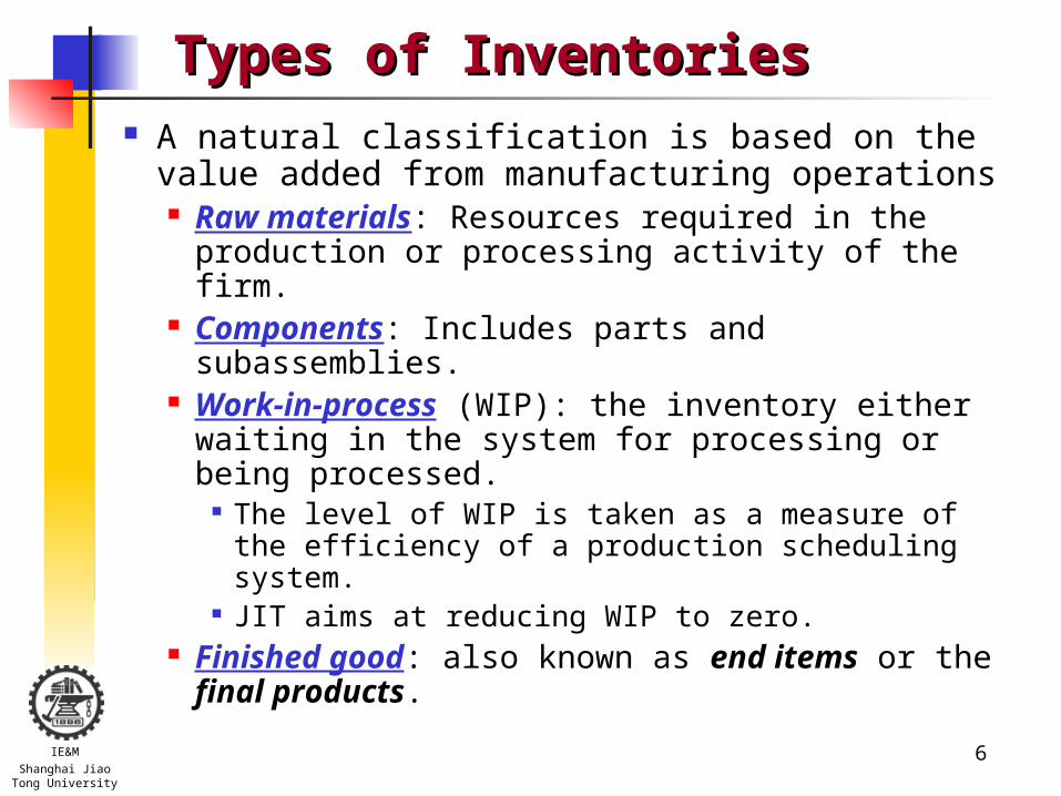
Types of InventoriesTypes of Inventories A natural classification is based on the value added
from manufacturing operations Raw materials: Resources required in the production
or processing activity of the firm. Components: Includes parts and subassemblies. Work-in-process (WIP): the inventory either waiting
in the system for processing or being processed. The level of WIP is taken as a measure of the
efficiency of a production scheduling system. JIT aims at reducing WIP to zero.
Finished good: also known as end items or the final products.

7IE&MShanghai Jiao
Tong University
Why Hold Inventories (1)Why Hold Inventories (1) For economies of scale
It may be economical to produce a relatively large number of items in each production run and store them for future use.
Coping with uncertainties Uncertainty in demand Uncertainty in lead time Uncertainty in supply
For speculation Purchase large quantities at current low prices and
store them for future use. Cope with labor strike

8IE&MShanghai Jiao
Tong University
Why Hold Inventories (2)Why Hold Inventories (2) Transportation
Pipeline inventories is the inventory moving from point to point, e.g., materials moving from suppliers to a plant, from one operation to the next in a plant.
Smoothing Producing and storing inventory in anticipation of
peak demand helps to alleviate the disruptions caused by changing production rates and workforce level.
Logistics To cope with constraints in purchasing, production,
or distribution of items, this may cause a system maintain inventory.

9IE&MShanghai Jiao
Tong University
Characteristics of Inventory SystemsCharacteristics of Inventory Systems Demand (patterns and characteristics)
Constant versus variable Known versus random
Lead Time Ordered from the outside Produced internally
Review Continuous: e.g., supermarket Periodic: e.g., warehouse
Excess demand demand that cannot be filled immediately from stock backordered or lost.
Changing inventory Become obsolete: obsolescence

10IE&MShanghai Jiao
Tong University
Relevant Costs - Relevant Costs - Holding CostHolding Cost
Holding cost (carrying or inventory cost) The sum of costs that are proportional to the amount
of inventory physically on-hand at any point in time Some items of holding costs
Cost of providing the physical space to store the items
Taxes and insurance Breakage, spoilage, deterioration, and obsolescence Opportunity cost of alternative investment
Inventory cost fluctuates with time inventory as a function of time

11IE&MShanghai Jiao
Tong University
Relevant Costs - Relevant Costs - Holding CostHolding Cost
Inventory as a Function of Time

12IE&MShanghai Jiao
Tong University
Relevant Costs - Relevant Costs - Order CostOrder Cost
It depend on the amount of inventory that is ordered or produced.
Two components The fixed cost K: independent of size of order The variable cost c: incurred on per-unit basis
0 0;( )
0
if xC x
K cx if x

13IE&MShanghai Jiao
Tong University
Relevant Costs - Relevant Costs - Order CostOrder Cost
Order Cost Function

14IE&MShanghai Jiao
Tong University
Relevant Costs - Relevant Costs - Penalty CostPenalty Cost Also know as shortage cost or stock-out cost
The cost of not having sufficient stock on-hand to satisfy a demand when it occurs.
Two interprets Backorder case: include delay costs may be involved Lost-sale case: include “loss-of-goodwill” cost, a measure of
customer satisfaction Two approaches
Penalty cost, p, is charged per-unit basis. Each time a demand occurs that cannot be satisfied immediately,
a cost p is incurred independent of how long it takes to eventually fill the demand.
Charge the penalty cost on a per-unit-time basis.

15IE&MShanghai Jiao
Tong University
EOQ HistoryEOQ History
Introduced in 1913 by Ford W. Harris, “How Many Parts to Make at Once” Product types: A, B and C A-B-C-A-B-C: 6 times of setup A-A-B-B-C-C: 3 times of setup
A factory producing various products and switching between products causes a costly setup (wages, material and overhead). Therefore, a trade-off between setup cost and production lot size should be determined.
Early application of mathematical modeling to Scientific Management

16IE&MShanghai Jiao
Tong University
EOQ Modeling AssumptionsEOQ Modeling Assumptions
1. Production is instantaneous – there is no capacity constraint and the entire lot is produced simultaneously.
2. Delivery is immediate – there is no time lag between production and availability to satisfy demand.
3. Demand is deterministic – there is no uncertainty about the quantity or timing of demand.
4. Demand is constant over time – in fact, it can be represented as a straight line, so that if annual demand is 365 units this translates into a daily demand of one unit.
5. A production run incurs a fixed setup cost – regardless of the size of the lot or the status of the factory, the setup cost is constant.
6. Products can be analyzed singly – either there is only a single product or conditions exist that ensure separability of products.

17IE&MShanghai Jiao
Tong University
NotationNotation
demand rate (units per year)
c proportional order cost at c per unit ordered (dollars per unit)
K fixed or setup cost to place an order (dollars)
h holding cost (dollars per year); if the holding cost consists entirely of interest on money tied up in inventory, then h = ic where i is an annual interest rate.
Q the unknown size of the order or lot size

18IE&MShanghai Jiao
Tong University
Inventory vs Time in EOQ ModelInventory vs Time in EOQ Model
Q/ 2Q/ 3Q/ 4Q/
Q
Inve
nto
ry
Time
slope = -
Order cycle: T=Q/

19IE&MShanghai Jiao
Tong University
CostsCosts
Holding Cost:
Setup Costs: K per lot, so
The average annual cost:
2cost holdingunit
2cost holding annual
2inventory average
hQ
hQ
Q
,cost setupunit Q
K
Q
KhQQG
2)(
Q
Kcost setup annual

20IE&MShanghai Jiao
Tong University
MedEquip ExampleMedEquip Example
Small manufacturer of medical diagnostic equipment. Purchases standard steel “racks” into which components
are mounted. Metal working shop can produce (and sell) racks more
cheaply if they are produced in batches due to wasted time setting up shop.
MedEquip doesn't want to hold too much capital in inventory.
Question: how many racks should MedEquip order at once?

21IE&MShanghai Jiao
Tong University
MedEquip Example CostsMedEquip Example Costs
= 1000 racks per year
c = $250
K = $500 (estimated from supplier’s pricing)
h = i*c + floor space cost = (0.1)($250) + $10 =
$35 per unit per year

22IE&MShanghai Jiao
Tong University
Costs in EOQ ModelCosts in EOQ Model
0.00
2.00
4.00
6.00
8.00
10.00
12.00
14.00
16.00
18.00
20.00
0 100 200 300 400 500
Order Quantity (Q)
Co
st (
$/u
nit
)
hQ/2D
A/Qc
Y(Q)
Q* =169

23IE&MShanghai Jiao
Tong University
Economic Order QuantityEconomic Order Quantity
Q
KhQQG
2)(
16935
)1000)(500(2* Q MedEquip Solution
EOQ Square Root Formula
Solution (by taking derivative and setting equal to zero):
h
KQ
QifQ
KQG
Q
Kh
dQ
QdGQG
2
002
)(''
02
)()('
*
3
2
Since Q”>0 , G(Q) is convex function of Q

24IE&MShanghai Jiao
Tong University
Another ExampleAnother Example Example 2
Pencils are sold at a fairly steady rate of 60 per week; Pencils cost 2 cents each and sell for 15 cents each; Cost $12 to initiate an order, and holding costs are based on
annual interest rate of 25%. Determine the optimal number of pencils for the book store to
purchase each time and the time between placement of orders Solutions
Annual demand rate =6052=3,120; The holding cost is the product of the variable cost of the
pencil and the annual interest-h=0.02 0.25=0.05
* 2 2 12 3,1203,870
0.05
KQ
h
3,8701.24
3,120
QT yr

25IE&MShanghai Jiao
Tong University
The EOQ Model-The EOQ Model-Considering Lead TimeConsidering Lead Time
Since there exists lead time (4 moths for Example 2), order should be placed some time ahead of the end of a cycle;
Reorder point R-determines when to place order in term of inventory on hand, rather than time.
Reorder Point Calculation for Example 2
26IE&MShanghai Jiao
Tong University
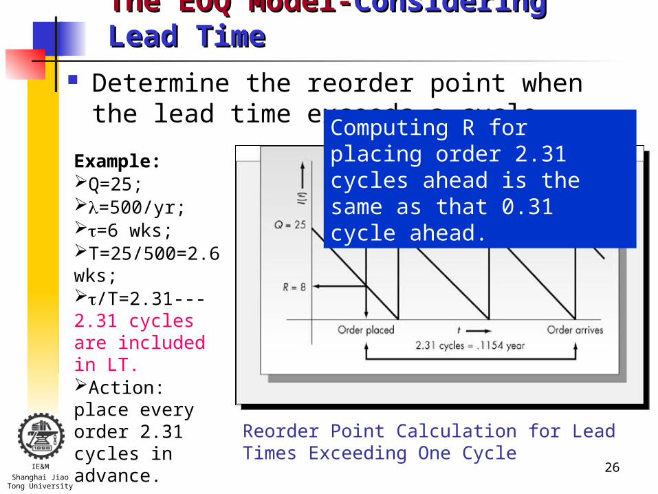
The EOQ Model-The EOQ Model-Considering Lead TimeConsidering Lead Time Determine the reorder point when the lead time
exceeds a cycle.
Example:Q=25;=500/yr;=6 wks;T=25/500=2.6 wks;/T=2.31---2.31 cycles are included in LT.Action: place every order 2.31 cycles in advance.
Reorder Point Calculation for Lead Times Exceeding One Cycle
Computing R for placing order 2.31 cycles ahead is the same as that 0.31 cycle ahead.

27IE&MShanghai Jiao
Tong University
EOQ Modeling AssumptionsEOQ Modeling Assumptions
1. Production is instantaneous – there is no capacity constraint and the entire lot is produced simultaneously.
2. Delivery is immediate – there is no time lag between production and availability to satisfy demand.
3. Demand is deterministic – there is no uncertainty about the quantity or timing of demand.
4. Demand is constant over time – in fact, it can be represented as a straight line, so that if annual demand is 365 units this translates into a daily demand of one unit.
5. A production run incurs a fixed setup cost – regardless of the size of the lot or the status of the factory, the setup cost is constant.
6. Products can be analyzed singly – either there is only a single product or conditions exist that ensure separability of products.
relax via EOQ Model for Finite Production Rate

28IE&MShanghai Jiao
Tong University
The EOQ Model for Finite Production RateThe EOQ Model for Finite Production Rate
The EOQ model with finite production rate is a variation of the basic EOQ model
Inventory is replenished gradually as the order is produced (which requires the production rate to be greater than the demand rate)
Notice that the peak inventory is lower than Q since we are using items as we produce them

29IE&MShanghai Jiao
Tong University
Notation – Notation – EOQ Model for Finite Production RateEOQ Model for Finite Production Rate
demand rate (units per year)
P production rate (units per year), where P>
c unit production cost, not counting setup or inventory costs (dollars per unit)
K fixed or setup cost (dollars)
h holding cost (dollars per year); if the holding cost is consists entirely of interest on money tied up in inventory, then h = ic where i is an annual interest rate.
Q the unknown size of the production lot size decision variable

30IE&MShanghai Jiao
Tong University
Inventory vs TimeInventory vs Time
Inve
nto
ry
Time
- P-
1. Production run of Q takes Q/P time units
(P-)(Q/P)
(P-)(Q/P)/2
2. When the inventory reaches 0, production begins until Q products are produced (it takes Q/P time units). During the Q/P time units, the inventory level will increases to (P-)(Q/P)
Inventory increase rate
Time
slope = -
slope = P-

31IE&MShanghai Jiao
Tong University
Solution to Solution to EOQ Model with Finite Production RateEOQ Model with Finite Production Rate
Annual Cost Function:
Solution (by taking first derivative and setting equal to zero):
2
)/1()(
QPh
Q
KQG
setup holding
)/1(
2*
Ph
KQ
• tends to EOQ as P
• otherwise larger than EOQ because replenishment takes longer
h
KQ
2* EOQ model
00
2
2
dQ
QGd
dQ
QdG

32IE&MShanghai Jiao
Tong University
Example: Non-Slip Tile Co.Example: Non-Slip Tile Co.
Non-Slip Tile Company (NST) has been using production runs of 100,000 tiles, 10 times per year to meet the demand of 1,000,000 tiles annually. The set-up cost is $5000 per run and holding cost is estimated at 10% of the manufacturing cost of $1 per tile. The production capacity of the machine is 500,000 tiles per month. The factory is open 365 days per year.

33IE&MShanghai Jiao
Tong University
Example: Non-Slip Tile Co. (Cont.)Example: Non-Slip Tile Co. (Cont.)
This is a “EOQ Model with Finite Production Rate” problem with = 1,000,000
P = 500,000*12 = 6,000,000
h = 0.1
K = 5,000

34IE&MShanghai Jiao
Tong University
Example: Non-Slip Tile Co. (Cont.)Example: Non-Slip Tile Co. (Cont.)
Find the Optimal Production Lot Size
How many runs should they expect per year?
How much will they save annually using EOQ Model with Finite Production Rate?

35IE&MShanghai Jiao
Tong University
Example: Non-Slip Tile Co. (Cont.)Example: Non-Slip Tile Co. (Cont.)
Optimal Production Lot Size
346410)6000000/10000001(1.0
)1000000)(5000(2
)/1(
2*
Ph
KQ
Number of Production Runs Per Year The number of runs per year = /Q* = 2.89 times per year

36IE&MShanghai Jiao
Tong University
Example: Non-Slip Tile Co. (Cont.)Example: Non-Slip Tile Co. (Cont.)
Annual Savings:
**1
Q
KhQ
PTC
Setupcost
Holdingcost
TC = 0.04167Q + 5,000,000,000/Current TC = 0.04167(1,000,000) + 5,000,000,000/(1,000,000)
= $54,167
Optimal TC = 0.04167(346,410) + 5,000,000,000/(346,410)
= $28,868
Difference = $54,167 - $28,868 = $25,299

37IE&MShanghai Jiao
Tong University
Sensitivity of EOQ Model to QuantitySensitivity of EOQ Model to Quantity
Optimal Unit Cost:
Optimal Annual Cost: Multiply G* by and simplify,
hK
K
hK
KhKh
Q
KhQQGG
2
2
22
2
2)(
*
***
hK2Cost Annual

38IE&MShanghai Jiao
Tong University
Sensitivity of EOQ Model to Quantity (cont.)Sensitivity of EOQ Model to Quantity (cont.)
Annual Cost from Using Q':
Ratio:
Q
KQhQG
2)(
Q
Q
Q
Q
hK
QKQh
QY
QY
Q
Q
*
*
**
2
1
......2
2
)(
)(
)(Cost
)(Cost

39IE&MShanghai Jiao
Tong University
Sensitivity of EOQ Model to Quantity (cont.)Sensitivity of EOQ Model to Quantity (cont.)
Q
Q
Q
Q
Q
Q *
** 2
1
)(Cost
)(Cost
Example: If Q' = 2Q*, then the ratio of the actual cost to optimal cost is
(1/2)[2 + (1/2)] = 1.25
If Q' = Q*/2, then the ratio of the actual cost to optimal cost is
(1/2)[(1/2)+2] = 1.25
A 100% error in lot size results in a 25% error in cost.

40IE&MShanghai Jiao
Tong University
EOQ TakeawaysEOQ Takeaways
Batching causes inventory (i.e., larger lot sizes translate into more stock).
Under specific modeling assumptions the lot size that optimally balances holding and setup costs is given by the square root formula:
Total cost is relatively insensitive to lot size (so rounding for other reasons, like coordinating shipping, may be attractive).
h
ADQ
2*

41IE&MShanghai Jiao
Tong University
Inventory Control Inventory Control Part 2 Inventory Control Subject to Part 2 Inventory Control Subject to
Unknown DemandUnknown Demand
By Ming DongBy Ming Dong
Department of Industrial Engineering & ManagementDepartment of Industrial Engineering & Management
Shanghai Jiao Tong UniversityShanghai Jiao Tong University

42IE&MShanghai Jiao
Tong University
The Wagner-Whitin Model
Change is not made without inconvenience, even from worse to better.
– Robert Hooker

43IE&MShanghai Jiao
Tong University
EOQ AssumptionsEOQ Assumptions
1. Instantaneous production.
2. Immediate delivery.
3. Deterministic demand.
4. Constant demand.
5. Known fixed setup costs.
6. Single product or separable products.
WW model relaxes this one

44IE&MShanghai Jiao
Tong University
Dynamic Lot Sizing NotationDynamic Lot Sizing Notationt a period (e.g., day, week, month); we will consider t = 1, … ,T,
where T represents the planning horizon.
Dt demand in period t (in units)
ct unit production cost (in dollars per unit), not counting setup or inventory costs in period t
At fixed or setup cost (in dollars) to place an order in period t
ht holding cost (in dollars) to carry a unit of inventory from period t to period t +1
Qt the unknown size of the order or lot size in period t
decision variables

45IE&MShanghai Jiao
Tong University
Wagner-Whitin ExampleWagner-Whitin Example
Data
Lot-for-Lot Solution
t 1 2 3 4 5 6 7 8 9 10Dt 20 50 10 50 50 10 20 40 20 30ct 10 10 10 10 10 10 10 10 10 10At 100 100 100 100 100 100 100 100 100 100ht 1 1 1 1 1 1 1 1 1 1
t 1 2 3 4 5 6 7 8 9 10 TotalDt 20 50 10 50 50 10 20 40 20 30 300Qt 20 50 10 50 50 10 20 40 20 30 300It 0 0 0 0 0 0 0 0 0 0 0Setup cost 100 100 100 100 100 100 100 100 100 100 1000Holding cost 0 0 0 0 0 0 0 0 0 0 0Total cost 100 100 100 100 100 100 100 100 100 100 1000
Since production cost c is constant, it can be ignored.

46IE&MShanghai Jiao
Tong University
Wagner-Whitin Example (cont.)Wagner-Whitin Example (cont.)
Fixed Order Quantity Solution
t 1 2 3 4 5 6 7 8 9 10 TotalDt 20 50 10 50 50 10 20 40 20 30 300Qt 100 0 0 100 0 0 100 0 0 0 300It 80 30 20 70 20 10 90 50 30 0 0Setup cost 100 0 0 100 0 0 100 0 0 0 300Holding cost 80 30 20 70 20 10 90 50 30 0 400Total cost 180 30 20 170 20 10 190 50 30 0 700
t 1 2 3 4 5 6 7 8 9 10Dt 20 50 10 50 50 10 20 40 20 30ct 10 10 10 10 10 10 10 10 10 10At 100 100 100 100 100 100 100 100 100 100ht 1 1 1 1 1 1 1 1 1 1
Data

47IE&MShanghai Jiao
Tong University
Wagner-Whitin PropertyWagner-Whitin Property
Under an optimal lot-sizing policy
(1) either the inventory carried to period t+1 from a previous period will be zero (there is a production in t+1)
(2) or the production quantity in period t+1 will be zero (there is no production in t+1)
A key observationIf we produce items in t (incur a setup cost) for use to satisfy demand in t+1, then it cannot possibly be economical to produce in t+1 (incur another setup cost) .
Either it is cheaper to produce all of period t+1’s demand in period t, or all of it in t+1; it is never cheaper to produce some in each.
Does fixed order quantity solution violate this property? Why?

48IE&MShanghai Jiao
Tong University
Basic Idea of Wagner-Whitin AlgorithmBasic Idea of Wagner-Whitin Algorithm
By WW Property, either Qt=0 or Qt=D1+…+Dk for some k.
If jk* = last period of production in a k period problem,
then we will produce exactly Dk+…DT in period jk*. Why?
We can then consider periods 1, … , jk*-1 as if they are an independent jk*-1 period problem.

49IE&MShanghai Jiao
Tong University
Wagner-Whitin ExampleWagner-Whitin Example
Step 1: Obviously, just satisfy D1 (note we are neglecting production cost, since it is fixed).
Step 2: Two choices, either j2* = 1 or j2* = 2.
1
100*1
1*1
j
AZ
1
150
200100100
150)50(1100min
2in produce ,Z
1in produce ,min
*2
2*1
211*2
j
A
DhAZ
t 1 2 3 4 5 6 7 8 9 10Dt 20 50 10 50 50 10 20 40 20 30ct 10 10 10 10 10 10 10 10 10 10At 100 100 100 100 100 100 100 100 100 100ht 1 1 1 1 1 1 1 1 1 1

50IE&MShanghai Jiao
Tong University
Wagner-Whitin Example (cont.)Wagner-Whitin Example (cont.)
Step3: Three choices, j3* = 1, 2, 3.
1
170
250 100150210 10)1(10010017010)11()50(1100
min
3in produce ,Z2in produce ,Z1in produce ,)(
min
*3
3*2
322*1
321211*3
j
ADhA
DhhDhAZ

51IE&MShanghai Jiao
Tong University
Wagner-Whitin Example (cont.)Wagner-Whitin Example (cont.)
Step 4: Four choices, j4* = 1, 2, 3, 4.
4
270
270 100170
300 50)1(100150
310 50)11(10)1(100100
32050)111(10)11()50(1100
min
4in produce ,Z
3in produce ,Z
2in produce ,)(Z
1in produce ,)()(
min
*4
4*3
433*2
432322*1
4321321211
*4
j
A
DhA
DhhDhA
DhhhDhhDhA
Z

52IE&MShanghai Jiao
Tong University
Planning Horizon PropertyPlanning Horizon Property
In the Example: Given fact: we produce in period 4 for period 4 of a 4 period
problem. Question: will we produce in period 3 for period 5 in a 5
period problem? Answer: We would never produce in period 3 for period 5 in
a 5 period problem.
If jt*=t, then the last period in which production occurs in an optimal t+1 period policy must be in the set t, t+1,…t+1. (this means that it CANNOT be t-1, t-2……)

53IE&MShanghai Jiao
Tong University
Wagner-Whitin Example (cont.)Wagner-Whitin Example (cont.) Step 5: Only two choices, j5* = 4, 5.
Step 6: Three choices, j6* = 4, 5, 6.
And so on.
4
320
370 100270
320)50(1100170min
5in produce ,Z
4in produce ,min
*5
5*4
544*3*
5
j
A
DhAZZ

54IE&MShanghai Jiao
Tong University
Wagner-Whitin Example SolutionWagner-Whitin Example Solution
Planning Horizon (t)Last Periodwith Production 1 2 3 4 5 6 7 8 9 10
1 100 150 170 3202 200 210 3103 250 3004 270 320 340 400 5605 370 380 420 5406 420 440 5207 440 480 520 6108 500 520 5809 580 610
10 620Zt 100 150 170 270 320 340 400 480 520 580
jt 1 1 1 4 4 4 4 7 7 or 8 8Produce in period 8 for 8, 9, 10 (40 + 20 + 30 = 90 units
Produce in period 4 for 4, 5, 6, 7 (50 + 50 + 10 + 20 = 130 units)
Produce in period 1 for 1, 2, 3 (20 + 50 + 10 = 80 units)

55IE&MShanghai Jiao
Tong University
Wagner-Whitin Example Solution (cont.)Wagner-Whitin Example Solution (cont.) Optimal Policy:
Produce in period 8 for 8, 9, 10 (40 + 20 + 30 = 90 units) Produce in period 4 for 4, 5, 6, 7 (50 + 50 + 10 + 20 = 130 units) Produce in period 1 for 1, 2, 3 (20 + 50 + 10 = 80 units)
t 1 2 3 4 5 6 7 8 9 10 Total Dt 20 50 10 50 50 10 20 40 20 30 300 Qt 80 0 0 130 0 0 0 90 0 0 300 It 60 10 0 80 30 20 0 50 30 0 0 Setup cost 100 0 0 100 0 0 0 100 0 0 300 Holding cost 60 10 0 80 30 20 0 50 30 0 280 Total cost 160 10 0 180 30 20 0 150 30 0 580

56IE&MShanghai Jiao
Tong University
Problems with Wagner-WhitinProblems with Wagner-Whitin
1. Fixed setup costs.
2. Deterministic demand and production (no uncertainty)
3. Never produce when there is inventory (WW Property). safety stock (don't let inventory fall to zero) random yields (can't produce for exact no. periods)
57IE&MShanghai Jiao
Tong University
Statistical Reorder Point Models
When your pills get down to four, Order more.
– Anonymous, from Hadley &Whitin

58IE&MShanghai Jiao
Tong University
EOQ AssumptionsEOQ Assumptions 1. Instantaneous production.
2. Immediate delivery.
3. Deterministic demand.
4. Constant demand.
5. Known fixed setup costs.
6. Single product or separable products.
WW model relaxes this one
newsvendor and (Q,r) relax this one
can use constraint approach
Chapter 17 extends (Q,r) to multiple product cases
lags can be added to EOQ or other models
EPL model relaxes this one

59IE&MShanghai Jiao
Tong University
Modeling Philosophies for Handling UncertaintyModeling Philosophies for Handling Uncertainty
1. Use deterministic model – adjust solution
- EOQ to compute order quantity, then add safety stock
- deterministic scheduling algorithm, then add safety lead time
2. Use stochastic model- news vendor model
- base stock and (Q,r) models
- variance constrained investment models

60IE&MShanghai Jiao
Tong University
The Newsvendor ApproachThe Newsvendor Approach Assumptions:
1. single period 2. random demand with known distribution 3. linear overage/shortage costs 4. minimum expected cost criterion
Examples: newspapers or other items with rapid obsolescence Christmas trees or other seasonal items

61IE&MShanghai Jiao
Tong University
Newsvendor Model NotationNewsvendor Model Notation
ariable.decision v theis thisunits);(in quantity /order production
shortage. ofunit per dollars)(in cost
realized. is demandafter over left unit per dollars)(in cost
demand. offunction density )()(
.)continuous (assumed
demand offunction on distributi cumulative ),()(
variable.random a units),(in demand
Q
c
c
xGdx
dxg
xXPxG
X
s
o

62IE&MShanghai Jiao
Tong University
Newsvendor ModelNewsvendor Model
Cost Function:
Qs
Q
o
so
so
dxxgQxcdxxgxQc
dxxgQxcdxxgxQc
EcEc
QY
)()()()(
)(0,max)(0,max
short unitsover units
cost shortage expected overage expected)(
0
00
Units over = max {Q-X, 0}
Units short = max {X-Q, 0}
Objective: find the value of Q that minimizes this expected cost.

63IE&MShanghai Jiao
Tong University
Newsvendor Model – Newsvendor Model – Leibnitz’s ruleLeibnitz’s rule
For Y(Q): taking its derivative and setting it to 0.To do this, we need to take the derivative of integrals with limits that
are functions of Q. A tool called Leibnitz's rule can do this.
)(
)(
11
22
)(
)(
2
1
2
1
)()),((
)()),(()],([),(
Qa
Qa
Qa
Qa dQ
QdaQQaf
dQ
QdaQQafdxQxf
QdxQxf
dQ
d
Applying this for Y(Q):
0)](1[)()()1()(1)(
00
0
QGcQGcdxxgcdxxgcdQ
QdYs
Qs
Q
so
s
cc
cQG
)( *

64IE&MShanghai Jiao
Tong University
Newsvendor Model (cont.)Newsvendor Model (cont.)
so
s
cc
cQXPQG
** )(
G(Q*) represents the probability that demand is less than or equal to Q*.
G(x)1
so
s
cc
c
Q*
Note:
Critical Ratio is thatprobability stockcovers demand
*
*
Qc
Qc
s
o
65IE&MShanghai Jiao
Tong University
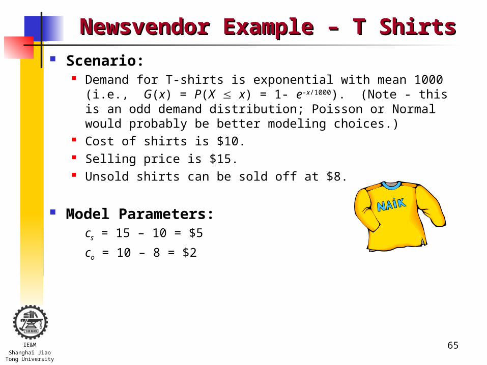
Newsvendor Example – T ShirtsNewsvendor Example – T Shirts Scenario:
Demand for T-shirts is exponential with mean 1000 (i.e., G(x) = P(X x) = 1- e-x/1000). (Note - this is an odd demand distribution; Poisson or Normal would probably be better modeling choices.)
Cost of shirts is $10. Selling price is $15. Unsold shirts can be sold off at $8.
Model Parameters:cs = 15 – 10 = $5
co = 10 – 8 = $2

66IE&MShanghai Jiao
Tong University
Newsvendor Example – T Shirts (cont.)Newsvendor Example – T Shirts (cont.)
Solution:
Sensitivity: If co = $10 (i.e., shirts must be discarded) then
253,1
714.052
51)(
*
1000*
Q
cc
ceQG
so
sQ
405
333.0510
51)(
*
1000*
Q
cc
ceQG
so
sQ
67IE&MShanghai Jiao
Tong University
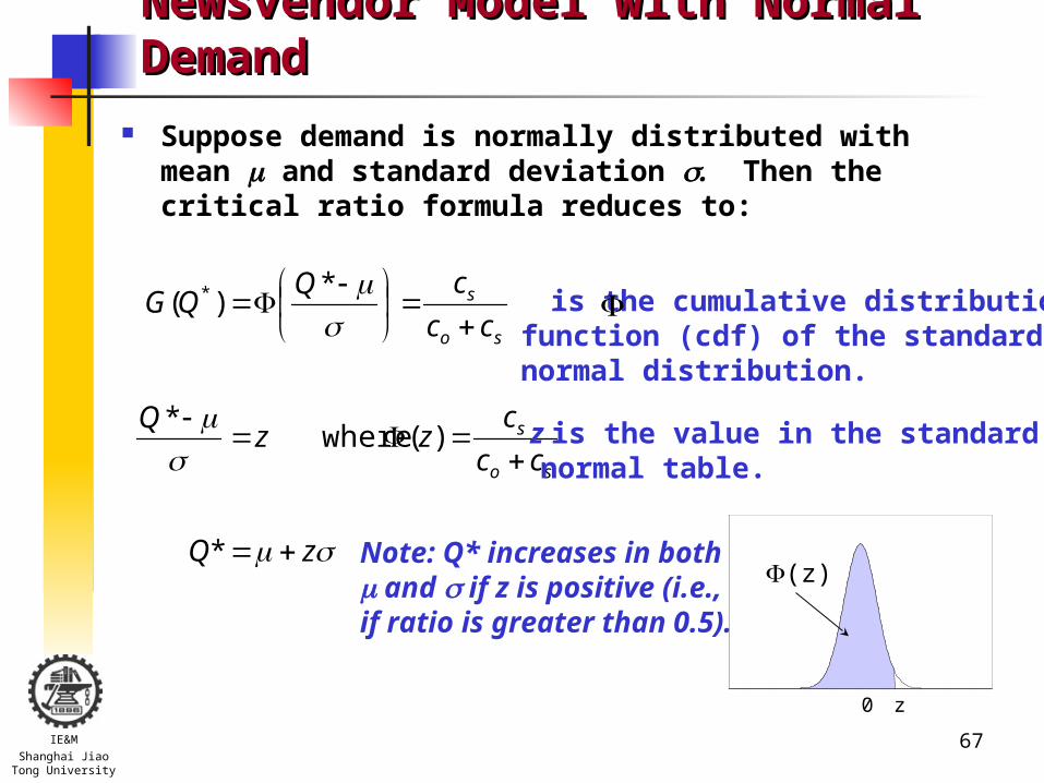
Newsvendor Model with Normal DemandNewsvendor Model with Normal Demand
Suppose demand is normally distributed with mean and standard deviation . Then the critical ratio formula reduces to:
Note: Q* increases in both and if z is positive (i.e.,if ratio is greater than 0.5).
zQ
cc
czz
Q
cc
cQQG
so
s
so
s
*
)( where*
*)( *
z00.00
3.00
1 7 13 19 25 31 37 43 49 55 61 67 73 79 85 91 97 103 109 115 121 127 133 139 145 151 157
(z)
is the cumulative distribution function (cdf) of the standard normal distribution.
z is the value in the standard normal table.
68IE&MShanghai Jiao
Tong University
Multiple Period ProblemsMultiple Period Problems
Difficulty: Technically, Newsvendor model is for a single period.
Extensions: But Newsvendor model can be applied to multiple period situations, provided: demand during each period is iid distributed according to
G(x) there is no setup cost associated with placing an order stockouts are either lost or backordered
Key: make sure co and cs appropriately represent overage and shortage cost.

69IE&MShanghai Jiao
Tong University
ExampleExample Scenario:
GAP orders a particular clothing item every Friday mean weekly demand is 100, std dev is 25 wholesale cost is $10, retail is $25 holding cost has been set at $0.5 per week (to reflect obsolescence,
damage, etc.)
Problem: how should they set order amounts?

70IE&MShanghai Jiao
Tong University
Example (cont.)Example (cont.)
Newsvendor Parameters: c0 = $0.5
cs = $15
Solution:
146)25(85.1100
85.125
100
9677.025
100
9677.0155.0
15)( *
Q
Q
Q
QG
Every Friday, they shouldorder-up-to 146, that is, ifthere are x on hand, then order 146-x.

71IE&MShanghai Jiao
Tong University
Newsvendor TakeawaysNewsvendor Takeaways
Inventory is a hedge against demand uncertainty.
Amount of protection depends on “overage” and “shortage” costs, as well as distribution of demand.
If shortage cost exceeds overage cost, optimal order quantity generally increases in both the mean and standard deviation of demand.

72IE&MShanghai Jiao
Tong University
The (The (QQ, , rr) Approach) Approach
Decision Variables:Reorder Point: r – affects likelihood of stockout
(safety stock).Order Quantity: Q – affects order frequency (cycle
inventory).
Assumptions:1. Continuous review of inventory.
2. Demands occur one at a time.
3. Unfilled demand is backordered.
4. Replenishment lead times are fixed and known.

73IE&MShanghai Jiao
Tong University
Inventory vs Time in (Inventory vs Time in (QQ,,rr) Model) Model
Q
Inve
nto
ry
Time
r
l
Delivery lead time

74IE&MShanghai Jiao
Tong University
The Base-Stock PolicyThe Base-Stock Policy
Start with an initial amount of inventory R. Each time a new demand arrives, place a replenishment order with the supplier.
An order placed with the supplier is delivered l units of time after it is placed.
Because demand is stochastic, we can have multiple orders that have been placed but not delivered yet.

75IE&MShanghai Jiao
Tong University
Base Stock ModelBase Stock Model
What the policy looks like Choose a base-stock level stock level R Each period, order to bring inventory position up to
the base-stock level R That order will arrive after a lead time l Costs are incurred based on net inventory Balance holding costs vs. backorder costs
76IE&MShanghai Jiao
Tong University
Base Stock Model AssumptionsBase Stock Model Assumptions
1. There is no fixed cost associated with placing an order.
2. There is no constraint on the number of orders that can be placed per year.
That is, we can replenishone at a time (Q=1).

77IE&MShanghai Jiao
Tong University
Base Stock NotationBase Stock Notation Q = 1, order quantity (fixed at one) r = reorder point R = r +1, base stock level l = delivery lead time = mean demand during l = std dev of demand during l p(x) = Prob{demand during lead time l equals x} G(x) = Prob{demand during lead time l is less than
x} h = unit holding cost b = unit backorder cost S(R) = average fill rate (service level) B(R) = average backorder level I(R) = average on-hand inventory level

78IE&MShanghai Jiao
Tong University
Inventory Balance EquationsInventory Balance Equations
Balance Equation:inventory position = on-hand inventory - backorders + orders
Under Base Stock Policy inventory position = R
On-hand inventory
On-order quantity from suppliers
Back-orders from customers
Inventory position R

79IE&MShanghai Jiao
Tong University
Inventory Profile for Base Stock System (Inventory Profile for Base Stock System (RR=5)=5)
0
1
2
3
4
5
6
7
0 5 10 15 20 25 30 35
Time
On Hand Inventory
Backorders
Orders
Inventory Position
l
R
r
# of orders = # of demands

80IE&MShanghai Jiao
Tong University
Service Level (Fill Rate)Service Level (Fill Rate)
Let:
X = (random) demand during lead time l
so E[X] = . Consider a specific replenishment order. Since inventory position is always R, the only way this item can stock out is if X R.
Expected Service Level:
discrete is if ),()1(
continuous is if ),()()(
GrGRG
GRGRXPRS

81IE&MShanghai Jiao
Tong University
Backorder LevelBackorder Level Note: At any point in time, number of orders equals number demands
that have occurred during the last l time units, (X), so from our previous balance equation:
R = on-hand inventory - backorders + orderson-hand inventory - backorders = R - X
Note: on-hand inventory and backorders are never positive at the same time, so if X=x, then
Expected Backorder Level:
RxRx
Rx
if ,
if ,0backorders
)](1)[()()()()( RGRRpxpRxRBRx
simpler version forspreadsheet computing
82IE&MShanghai Jiao
Tong University
Inventory LevelInventory Level
Observe:
on-hand inventory - backorders = R-X
E[X] =
E[backorders] = B(R) from previous slide
Result:I(R) = R - + B(R)

83IE&MShanghai Jiao
Tong University
Base Stock ExampleBase Stock Example
l = one month
= 10 units (per month)
Assume Poisson demand, so
x
k
x
k
k
k
ekpxG
0 0
10
!
10)()( Note: Poisson
demand is a good choice when no variability data is available.

84IE&MShanghai Jiao
Tong University
Base Stock Example CalculationsBase Stock Example Calculations
R p(R) G(R) B(R) R p(R) G(R) B(R)0 0.000 0.000 10.000 12 0.095 0.792 0.5311 0.000 0.000 9.000 13 0.073 0.864 0.3222 0.002 0.003 8.001 14 0.052 0.917 0.1873 0.008 0.010 7.003 15 0.035 0.951 0.1034 0.019 0.029 6.014 16 0.022 0.973 0.0555 0.038 0.067 5.043 17 0.013 0.986 0.0286 0.063 0.130 4.110 18 0.007 0.993 0.0137 0.090 0.220 3.240 19 0.004 0.997 0.0068 0.113 0.333 2.460 20 0.002 0.998 0.0039 0.125 0.458 1.793 21 0.001 0.999 0.00110 0.125 0.583 1.251 22 0.000 0.999 0.00011 0.114 0.697 0.834 23 0.000 1.000 0.000
Summarize the results in Table

85IE&MShanghai Jiao
Tong University
Base Stock Example ResultsBase Stock Example Results
Service Level: For fill rate of 90%, we must set R-1= r =14, so R=15 and safety stock s = r- = 4. Resulting service is 91.7%.
Backorder Level:
B(R) = B(15) = 0.103
Inventory Level:
I(R) = R - + B(R) = 15 - 10 + 0.103 = 5.103

86IE&MShanghai Jiao
Tong University
““Optimal” Base Stock LevelsOptimal” Base Stock Levels
Objective Function:
Y(R) = hI(R) + bB(R)
= h(R-+B(R)) + bB(R)
= h(R- ) + (h+b)B(R)
Solution: if we assume G is continuous, we can get
)( *
bh
bRG
Implication: set base stocklevel so fill rate is b/(h+b).
Note: R* increases in b anddecreases in h.
holding plus backorder cost

87IE&MShanghai Jiao
Tong University
Base Stock Normal ApproximationBase Stock Normal Approximation
If G is normal(,), then
where (z)=b/(h+b). So
R* = + z
zR
bh
bRG
*
*)(
Note: R* increases in and also increases in provided z>0.
z is the value from the standard normal table.

88IE&MShanghai Jiao
Tong University
““Optimal” Base Stock ExampleOptimal” Base Stock Example
Data: Approximate Poisson with mean 10 by normal with mean 10 units/month and standard deviation 10 = 3.16 units/month. Set h=$15, b=$25.
Calculations:
since (0.32) = 0.625, z=0.32 and hence
R* = + z = 10 + 0.32(3.16) = 11.01 11
Observation: from previous table fill rate is G(10) = 0.583, so maybe backorder cost is too low.
0.6252515
25
bh
b

89IE&MShanghai Jiao
Tong University
Inventory PoolingInventory Pooling
Situation: n different parts with lead time demand normal(, ) z=2 for all parts (i.e., fill rate is around 97.5%)
Specialized Inventory: base stock level for each item = + 2 total safety stock = 2n
Pooled Inventory: suppose parts are substitutes for one another lead time demand is normal (n ,n ) base stock level (for same service) = n +2 n ratio of safety stock to specialized safety stock = 1/ n
cycle stock safety stock

90IE&MShanghai Jiao
Tong University
Effect of Pooling on Safety StockEffect of Pooling on Safety Stock
Conclusion: cycle stock isnot affected by pooling, butsafety stock falls dramatically.So, for systems with high safetystock, pooling (through productdesign, late customization, etc.)can be an attractive strategy.

91IE&MShanghai Jiao
Tong University
Pooling ExamplePooling Example
PC’s consist of 6 components (CPU, HD, CD ROM, RAM, removable storage device, keyboard)
3 choices of each component:
Each component costs $150 ($900 material cost per PC)
Demand for all models is Poisson distributed with mean 100 per year
Replenishment lead time is 3 months (0.25 years)
Use base stock policy with fill rate of 99%
36 = 729 different PC’s

92IE&MShanghai Jiao
Tong University
Pooling Example - Stock PC’sPooling Example - Stock PC’s
Base Stock Level for Each PC: = 100 0.25 = 25, so using Poisson formulas,
G(R-1) 0.99 R = 38 units
On-Hand Inventory for Each PC:
I(R) = R - + B(R) = 38 - 25 + 0.0138 = 13.0138 units
Total On-Hand Inventory:
13.0138 729 $900 = $8,538,358

93IE&MShanghai Jiao
Tong University
Pooling Example - Stock ComponentsPooling Example - Stock Components Necessary Service for Each Component: S = (0.99)1/6 = 0.9983
Base Stock Level for Components: = (100 729/3)0.25 = 6075, so G(R-1) 0.9983 R = 6306
On-Hand Inventory Level for Each Component:
I(R) = R - + B(R) = 6306-6075+0.0363 = 231.0363 units
Total On-Hand Inventory:
231.0363 18 $150 = $623,798
93% reduction!
729 models of PC3 types of each comp.

94IE&MShanghai Jiao
Tong University
Base Stock InsightsBase Stock Insights
1. Reorder points control prob of stockouts by establishing safety stock.
2. To achieve a given fill rate, the required base stock level (and hence safety stock) is an increasing function of mean and (provided backorder cost exceeds shortage cost) std dev of demand during replenishment lead time.
3. The “optimal” fill rate is an increasing in the backorder cost and a decreasing in the holding cost. We can use either a service constraint or a backorder cost to determine the appropriate base stock level.
4. Base stock levels in multi-stage production systems are very similar to kanban systems and therefore the above insights apply.
5. Base stock model allows us to quantify benefits of inventory pooling.
95IE&MShanghai Jiao
Tong University
The Single Product (The Single Product (QQ,,rr) Model) Model
Motivation: Either
1. Fixed cost associated with replenishment orders and cost per backorder.
2. Constraint on number of replenishment orders per year and service constraint.
Objective: Under (1)
costbackorder cost holdingcost setup fixed min Q,r
As in EOQ, this makesbatch production attractive.

96IE&MShanghai Jiao
Tong University
Summary of (Q,r) Model AssumptionsSummary of (Q,r) Model Assumptions
1. One-at-a-time demands.
2. Demand is uncertain, but stationary over time and distribution is known.
3. Continuous review of inventory level.
4. Fixed replenishment lead time.
5. Constant replenishment batch sizes.
6. Stockouts are backordered.

97IE&MShanghai Jiao
Tong University
(Q,r)(Q,r) Notation Notation
cost backorder unit annual
stockoutper cost
cost holdingunit annual
iteman ofcost unit
orderper cost fixed
timelead during demand of cdf ) ()(
timelead during demand of pmf )(
timeleadent replenishm during demand ofdeviation standard
timeleadent replenishm during demand expected ][
timeleadent replenishm during demand (random)
constant) (assumed timeleadent replenishm
yearper demand expected
b
k
h
c
A
xXPxG
xXPp(x)
XE
X
D

98IE&MShanghai Jiao
Tong University
(Q,r)(Q,r) Notation (cont.) Notation (cont.)
levelinventory average),(
levelbackorder average ),(
rate) (fill level service average ),(
frequencyorder average )(
by impliedstock safety
pointreorder
quantityorder
rQI
rQB
rQS
QF
rrs
r
Q
Decision Variables:
Performance Measures:

99IE&MShanghai Jiao
Tong University
Inventory and Inventory Position for Inventory and Inventory Position for QQ=4, =4, rr=4=4
-2
-1
0
1
2
3
4
5
6
7
8
9
0 2 4 6 8 10 12 14 16 18 20 22 24 26 28 30 32
Time
Qu
anti
ty
Inventory Position Net Inventory
Inventory Positionuniformly distributedbetween r+1=5 and r+Q=8

100IE&MShanghai Jiao
Tong University
Costs in Costs in (Q,r)(Q,r) Model Model
Fixed Setup Cost: AF(Q)
Stockout Cost: kD(1-S(Q,r)), where k is cost per stockout
Backorder Cost: bB(Q,r)
Inventory Carrying Costs: cI(Q,r)

101IE&MShanghai Jiao
Tong University
Fixed Setup Cost in (Fixed Setup Cost in (QQ,,rr) Model) Model
Observation: since the number of orders per year is D/Q,
Q
DF(Q)

102IE&MShanghai Jiao
Tong University
Stockout Cost in Stockout Cost in (Q,r)(Q,r) Model Model
Key Observation: inventory position is uniformly distributed between r+1 and r+Q. So, service in (Q,r) model is weighted sum of service in base stock model.
Result:
)]()([1
1),(
)]1()([1
)1(1
),(1
QrBrBQ
rQS
QrGrGQ
xGQ
rQSQr
rx
Note: this form is easier to use in spreadsheets because it does not involve a sum.
R
xRx
xGRBxpRxRB0
)](1[)()()()(

103IE&MShanghai Jiao
Tong University
Service Level ApproximationsService Level Approximations
Type I (base stock):
Type II:
)(),( rGrQS
Q
rBrQS
)(1),(
Note: computes numberof stockouts per cycle, underestimates S(Q,r)
Note: neglects B(r,Q)term, underestimates S(Q,r)

104IE&MShanghai Jiao
Tong University
Backorder Costs in (Backorder Costs in (QQ,,rr) Model) Model
Key Observation: B(Q,r) can also be computed by averaging base stock backorder level function over the range [r+1,r+Q]. (Similar to the fill rate)
Result:
Qr
rx
QrBrBQ
xBQ
rQB1
)]()1([1
)(1
),(
Notes: 1. B(Q,r) B(r) is a base stock approximation for backorder level.
2. If we can compute B(x) (base stock backorder level function), then we can compute stockout and backorder costs in (Q,r) model.

105IE&MShanghai Jiao
Tong University
Inventory Costs in (Inventory Costs in (QQ,,rr) Model) Model
Approximate Analysis: on average inventory declines from Q+s to s+1 so
Exact Analysis: this neglects backorders, which add to average inventory since on-hand inventory can never go below zero. The corrected version turns out to be
rQ
sQssQ
rQI2
1
2
1
2
)1()(),(
),(2
1),( rQBr
QrQI

106IE&MShanghai Jiao
Tong University
Inventory vs Time in (Inventory vs Time in (QQ,,rr) Model) Model
Inve
nto
ry
Time
r
s+1=r-+1
s+Q
Expected Inventory Actual Inventory
Approx I(Q,r)
Exact I(Q,r) =Approx I(Q,r) + B(Q,r)

107IE&MShanghai Jiao
Tong University
Expected Inventory Level for Expected Inventory Level for QQ=4, =4, rr=4, =4, =2=2
0
1
2
3
4
5
6
7
0 5 10 15 20 25 30 35
Time
Inve
nto
ry L
evel
s+Q
s

108IE&MShanghai Jiao
Tong University
(Q,r)(Q,r) Model with Backorder Cost Model with Backorder Cost
Objective Function:
Approximation: B(Q,r) makes optimization complicated because it depends on both Q and r. To simplify, approximate with base stock backorder formula, B(r):
),(),(),( rQhIrQbBAQ
DrQY
))(2
1()(),(
~),( rBr
QhrbBA
Q
DrQYrQY
109IE&MShanghai Jiao
Tong University
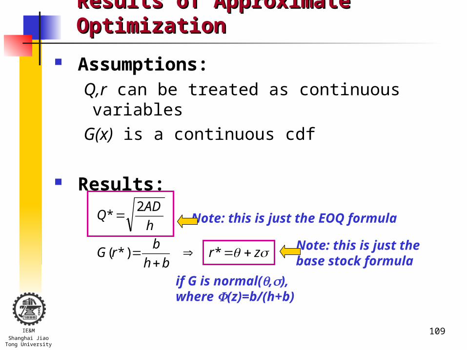
Results of Approximate OptimizationResults of Approximate Optimization
Assumptions: Q,r can be treated as continuous variables
G(x) is a continuous cdf
Results:
zrbh
brG
h
ADQ
**)(
2*
if G is normal(,),where (z)=b/(h+b)
Note: this is just the EOQ formula
Note: this is just the base stock formula
110IE&MShanghai Jiao
Tong University
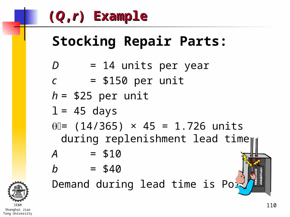
((QQ,,rr) Example) Example
Stocking Repair Parts:
D = 14 units per year
c = $150 per unit
h = $25 per unit
l = 45 days
= (14/365) × 45 = 1.726 units during replenishment lead time
A = $10
b = $40
Demand during lead time is Poisson

111IE&MShanghai Jiao
Tong University
Values for Poisson(Values for Poisson() Distribution) Distribution
111
r p(r) G(r) B(r)
0 0.178 0.178 1.7261 0.307 0.485 0.9042 0.265 0.750 0.3893 0.153 0.903 0.1404 0.066 0.969 0.0425 0.023 0.991 0.0116 0.007 0.998 0.0037 0.002 1.000 0.0018 0.000 1.000 0.0009 0.000 1.000 0.000
10 0.000 1.000 0.000

112IE&MShanghai Jiao
Tong University
Calculations for ExampleCalculations for Example
2107.2)314.1(29.0726.1*
29.0 so ,615.0)29.0(
615.04025
40
43.415
)14)(10(22*
zr
z
bh
b
h
ADQ

113IE&MShanghai Jiao
Tong University
Performance Measures for ExamplePerformance Measures for Example
823.2049.0726.122
14*)*,(*
2
1**)*,(
049.0]003.0011.0042.0140.0[4
1
)]6()5()4()3([1
)(*
1*)*,(
904.0]003.0389.0[4
11
)]42()2([1
1*)]*(*)([*
11**
5.34
14
**)(
**
1*
rQBrQ
rQI
BBBBQ
xBQ
rQB
BBQ
QrBrBQ
),rS(Q
Q
DQF
Qr
rx

114IE&MShanghai Jiao
Tong University
Observations on ExampleObservations on Example
Orders placed at rate of 3.5 per year
Fill rate fairly high (90.4%)
Very few outstanding backorders (0.049 on
average)
Average on-hand inventory just below 3 (2.823)

115IE&MShanghai Jiao
Tong University
Varying the ExampleVarying the Example
Change: suppose we order twice as often so F=7 per year, then Q=2 and:
which may be too low, so increase r from 2 to 3:
This is better. For this policy (Q=2, r=3) we can compute B(2,3)=0.026, I(Q,r)=2.80.
Conclusion: this has higher service and lower inventory than the original policy (Q=4, r=2). But the cost of achieving this is an extra 3.5 replenishment orders per year.
826.0]042.0389.0[2
11)]()([
11),( QrBrB
QrQS
936.0]011.0140.0[2
11)]()([
11),( QrBrB
QrQS

116IE&MShanghai Jiao
Tong University
(Q,r)(Q,r) Model with Stockout Cost Model with Stockout Cost
Objective Function:
Approximation: Assume we can still use EOQ to compute Q* but replace S(Q,r) by Type II approximation and B(Q,r) by base stock approximation:
),()),(1(),( rQhIrQSkDAQ
DrQY
))(2
1(
)(),(
~),( rBr
Qh
Q
rBkDA
Q
DrQYrQY

117IE&MShanghai Jiao
Tong University
Results of Approximate OptimizationResults of Approximate Optimization
Assumptions: Q,r can be treated as continuous variablesG(x) is a continuous cdf
Results:
zrhQkD
kDrG
h
ADQ
**)(
2*
if G is normal(,),where (z)=kD/(kD+hQ)
Note: this is just the EOQ formula
Note: another version of base stock formula(only z is different)

118IE&MShanghai Jiao
Tong University
Backorder vs. Stockout ModelBackorder vs. Stockout Model
Backorder Model when real concern is about stockout time because B(Q,r) is proportional to time customers wait for
backorders useful in multi-level systems
Stockout Model when concern is about fill rate better approximation of lost sales situations (e.g., retail)
Note: We can use either model to generate solutions Keep track of all performance measures regardless of model B-model will work best for backorders, S-model for stockouts

119IE&MShanghai Jiao
Tong University
Lead Time VariabilityLead Time Variability
Problem: replenishment lead times may be variable, which increases variability of lead time demand.
Notation:
L = replenishment lead time (days), a random variable
l = E[L] = expected replenishment lead time (days)
L= std dev of replenishment lead time (days)
Dt = demand on day t, a random variable, assumed
independent and identically distributed
d = E[Dt] = expected daily demand
D= std dev of daily demand (units)

120IE&MShanghai Jiao
Tong University
Including Lead Time Variability in FormulasIncluding Lead Time Variability in Formulas
Standard Deviation of Lead Time Demand:
Modified Base Stock Formula (Poisson demand case):
22222LLD dd
22LdzzR
Inflation term due tolead time variability
Note: can be used in anybase stock or (Q,r) formulaas before. In general, it willinflate safety stock.
if demand is Poisson

121IE&MShanghai Jiao
Tong University
Single Product (Single Product (QQ,,rr) Insights) Insights
Basic Insights: Safety stock provides a buffer against stockouts. Cycle stock increases as replenishment frequency decreases.
Other Insights:1. Increasing D tends to increase optimal order quantity Q.
2. Increasing tends to increase the optimal reorder point. (Note: either increasing D or l increases .)
3. Increasing the variability of the demand process tends to increase the optimal reorder point (provided z > 0).
4. Increasing the holding cost tends to decrease the optimal order quantity and reorder point.

122IE&MShanghai Jiao
Tong University
Safety StockSafety Stock
Stock carried to provide a level of protection against costly stockouts due to uncertainty of demand during lead time
Stock outs occur when Demand over the lead time is larger than
expected service level (1 - )100%.
Service LevelService Level
123IE&MShanghai Jiao
Tong University
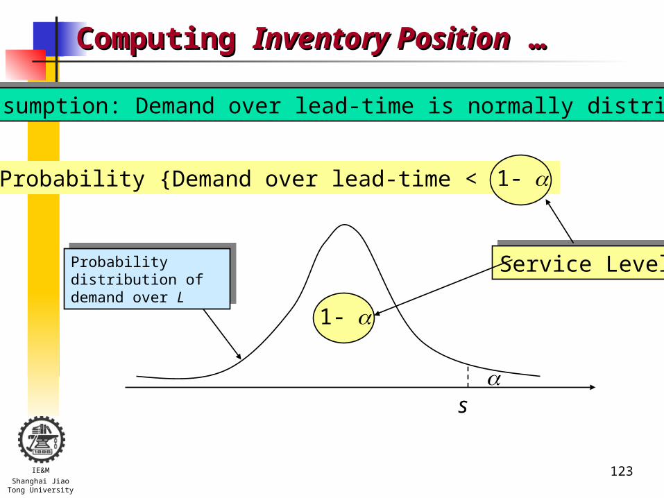
Computing Computing Inventory PositionInventory Position … …
Probability {Demand over lead-time < s} = 1-
Service LevelService Level
1-
Assumption: Demand over lead-time is normally distributedAssumption: Demand over lead-time is normally distributed
s
Probability distribution of demand over L
Probability distribution of demand over L

124IE&MShanghai Jiao
Tong University
Computing Computing Inventory PositionInventory Position: Normal Distribution: Normal Distribution
1-
s
Probability distribution of demand over L:
Mean = ; Std Dev =
Probability distribution of demand over L:
Mean = ; Std Dev =
sz s z
sz s z
1-
z0
1 - .90 .95 .98 .99 .999
z 1.28 1.65 2.05 2.33 3.09
From normal table or, in Excel, use: =normsinv (0.90)

125IE&MShanghai Jiao
Tong University
Computation of Variance for Demand over Lead Time:Computation of Variance for Demand over Lead Time:Variability Comes From Two SourcesVariability Comes From Two Sources
LD L AVG
2 2 2{ } { } { }LVar D Var L AVG AVG Var L AVG STDL
3: Adding the two terms, we get to our result
2 2 2{ }LVar D AVGL STD AVG STDL
1 2 ...L AVGLD d d d timesAVGL
1: Suppose only demand di in day i is variable; lead time is constant at AVGL
2: Now, suppose only lead time is variable; daily demand is constant at AVG
21 2 1 2{ } { ... } { } { } ... { }L AVGL AVGLVar D Var d d d Var d Var d Var d AVGL STD
di’s are independent di’s are identically distributed

126IE&MShanghai Jiao
Tong University
Safety stock SS
More specifically….More specifically….
2 2 2s AVG AVGL z STDL AVG STD AVGL
Note:•If lead time is constant,• If demand is constant,
0STDL 0STD
Standard deviation of demand over LT
Safety factor (std
normal table)
Mean demand over LT

127IE&MShanghai Jiao
Tong University
Example:Example: Consider inventory management for a certain SKU at
Home Depot. Supply lead time is variable (since it depends on order consolidation with other stores) and has a mean of 5 days and std deviation of 2 days. Daily demand for the item is variable with a mean of 30 units and std deviation of 6 units. Find the reorder point for 95% service level.
5; 2AVGL STDL
95% service level z = 1.64
2 2 2
2 2 2 30 5 1.64 2 30 6 5 150 100.8 251
s AVG AVGL z STDL AVG STD AVGL
AVG = 30, STD = 6

128IE&MShanghai Jiao
Tong University
The (s,S) Policy: Fixed Ordering CostsThe (s,S) Policy: Fixed Ordering Costs
s should be set to cover the lead time demand and together with a safety stock that insures the stock out probability is within the specific limit (When to reorder).
S depends on the fixed order cost – EOQ (How much)
Time
Inve
ntor
y
L
R
Orderplaced
Orderarrives
Average demandduring lead time
Safety Stock
sS

129IE&MShanghai Jiao
Tong University
The (s,S) Policy: Fixed Ordering CostsThe (s,S) Policy: Fixed Ordering Costs
Compute s exactly as in the base-stock model:
• Compute Q using the EOQ formula, using mean demand D = AVG (be careful about units…):
• Set S = s + Q
• Order when: inventory position (IP) drops below s• Order how much: bring IP to S
2 2 2s AVG AVGL z STDL AVG STD AVGL 2 2 2s AVG AVGL z STDL AVG STD AVGL
h
ADQ
2*

130IE&MShanghai Jiao
Tong University
Example: (s,S) ModelExample: (s,S) Model Consider previous Home Depot example, however, there
are fixed ordering costs, which are estimated at $50. Assume that holding costs are 15% of the product cost ($80) per year. Also, assume that the store is open 360 days a year.
2 2(30)50300
0.0333AVG K
Qh
251 300 551S s Q
251s (from previous calculations)
h = (0.15)*80/360=0.0333; A = K = 50, D = AVG = 30

131IE&MShanghai Jiao
Tong University
Summary of Inventory ModelsSummary of Inventory Models
Is demand rate and lead time constant?
Use EOQ•How much: EOQ formula•When: d*L
no
yesAre there fixed ordering costs?
no
yesUse (s, S) policy
•How much: Q = S – s (Q is from EOQ formula)•When: IP drops below s (base-stock policy formula)
Use base stock (s) policy•When: IP drops below s•How much: necessary to bring IP back to s