energies

Article

Computational Modeling of Gurney Flaps andMicrotabs by POD Method

Unai Fernandez-Gamiz 1,* ID , Macarena Gomez-Mármol 2 and Tomas Chacón-Rebollo 2,3

1 Nuclear Engineering and Fluid Mechanics Department, University Basque Country, UPV/EHU,01006 Vitoria, Spain

2 Department Ecuac Diferenciales & Anal Numer, Fac Mathematics, University Seville, 41012 Seville, Spain;macarena@us.es

3 Instituto de Matemáticas Universidad de Sevilla (IMUS), University Seville, 41012 Seville, Spain;chacon@us.es

* Correspondence: unai.fernandez@ehu.eus; Tel.: +34-945014066

Received: 6 July 2018; Accepted: 10 August 2018; Published: 11 August 2018

Abstract: Gurney flaps (GFs) and microtabs (MTs) are two of the most frequently used passive flowcontrol devices on wind turbines. They are small tabs situated close to the airfoil trailing edge andnormal to the surface. A study to find the most favorable dimension and position to improve theaerodynamic performance of an airfoil is presented herein. Firstly, a parametric study of a GF on aS810 airfoil and an MT on a DU91(2)250 airfoil was carried out. To that end, 2D computational fluiddynamic simulations were performed at Re = 106 based on the airfoil chord length and using RANSequations. The GF and MT design parameters resulting from the computational fluid dynamics(CFD) simulations allowed the sizing of these passive flow control devices based on the airfoil’saerodynamic performance. In both types of flow control devices, the results showed an increase in thelift-to-drag ratio for all angles of attack studied in the current work. Secondly, from the data obtainedby means of CFD simulations, a regular function using the proper orthogonal decomposition (POD)was used to build a reduced order method. In both flow control cases (GFs and MTs), the recursivePOD method was able to accurately and very quickly reproduce the computational results with verylow computational cost.

Keywords: wind energy; flow control; Gurney flaps; microtabs; proper orthogonal decomposition;reduced order method

1. Introduction

The significant increase of wind turbine size and weight in the past decade has made it impossibleto control them as they were 30 years ago. Wind turbine rotors of 140 m or even more are now a reality.Johnson et al. [1] compiled some of the most important load control techniques that can be used inwind turbines to ensure a safe and optimal operation under a diversity of atmospheric environments.These include blades made of soft, flexible materials that change shape in response to wind speed oraerodynamic loads, aerodynamically-shaped rotating towers, flexible rotor systems with hinged blades,and other advanced control systems. The larger the size of a wind turbine, the higher the structuraland fatigue loads, which affect the rotor and other key mechanisms of the turbine. A reduction of thesesevere loads can be achieved by developing novel load control techniques. Loads on wind turbinesare normally divided into extreme structural loads and fatigue loads. Reducing these fatigue loadsis a main goal, which can reduce the maintenance costs and improve the reliability of wind turbines(see Baek et al. [2]).

Energies 2018, 11, 2091; doi:10.3390/en11082091 www.mdpi.com/journal/energies

Energies 2018, 11, 2091 2 of 19

Several flow control systems were developed in the past decades. Most of them were created foraeronautical issues, and this was their first research field and application. Researchers are currentlyworking to optimize and introduce this type of device in wind turbines [3]. Wood [4] developed afour-layer scheme that allows classification of the diverse concepts. As explained in Aramendia et al. [5,6],they can be classified as actives or passives devices depending on their operating principle. To alleviateloads successfully, it is indispensable that the device to be able to reduce the generated lift. The studiespresented by Johnson et al. [7] and Frederick et al. [8] provide different ways of using this type of deviceto mitigate turbine loads.

Gurney flaps (GFs) were originally used for lift enhancement in the field of aeronautics [9,10].The advantages and limitations of these devices have been acutely documented [9,11]. The firstapplication was in racing cars, as small vertical strips attached to the trailing edge (TE) of the wing.The GF was first considered by Liebeck [12] and improved by Jeffrey et al. [13,14]. Tang and Dowell [15]compared the experimental loading of a NACA 0012 airfoil with both static and oscillating trailing-edgeGFs using an incompressible Navier–Stokes solver. A movable GF on a NACA 4412 airfoil wasstudied by Camocardi et al. [16], where the flow pattern behavior in the near wake of the airfoilwas investigated. Lee [17] also studied the impact of GFs of different sizes and perforations on thegrowth and development of the tip vortex generated by a NACA 0012 airfoil using particle imagevelocimetry (PIV). Recently, Cole et al. [18] studied the effect of GFs of different heights, and the resultsindicated that the airfoil shape is decisive in the aerodynamic performance of the airfoil with GFs.Recently, researchers have returned to GFs to study prospective benefits in rotorcrafts and helicoptersapplications [13–15]. Liu et al. [19] and Min et al. [20] used microflaps for vibration reduction inhelicopter rotors. Additionally, the influence of GFs on the power output performance of a 5 MWhorizontal axis wind turbine was investigated by Fernandez-Gamiz et al. [21]. Increments in theaverage power output of 10.4% and 3.5% were found at two different wind velocity realizations.GFs appear to be one of most appropriate devices to improve reliability and/or power output in largewind turbines.

Microtabs (MTs) are defined as small tabs situated near the trailing edge (TE) of an airfoil, andproject perpendicular to the surface of the airfoil by a few percent of the chord length (1–2% of c)corresponding to the boundary layer thickness. These MTs jet the flow in the boundary layer away fromthe airfoil surface, bringing a recirculation zone at the rear of the tab and affecting the aerodynamicbehavior, moving the flow separation zone and consequently changing the lift. The lift can be enhancedby deploying the MT on the pressure side of the airfoil; on the contrary the lift is reduced if the MTis deployed on the suction side. MT concept and flow around a trailing-edge region during tabpressure-side deployment can be found in Chow et al. [22]. Van Dam [23] carried out multiple studiesand investigations into this topic, including computational fluid dynamics (CFD) simulations andwind tunnel experiments, in order to determine their optimal distribution height and location. As inprevious studies, the results provided that the best place to situate the lower surface tab with respectto lift and drag was around 0.95 c with a height of 0.01 c and around 0.90 c for the upper surfacetab. MTs present some attractive features for wind turbine control applications, such as small size,design simplicity, and low set-up cost [24]. They can also be installed without significant changesin the actual techniques to manufacture the profiles. Tsai et al. [25] recently presented an innovativedesign to improve the MT performance. This new MT system is based on a four-bar linkage, providingan increase of the maximum tab height in relation to the existing MT system and better stability due tothe four-bar linkage mechanism. Furthermore, blade element momentum (BEM)-based computationswere performed in the study of Fernandez-Gamiz et al. [26] to investigate the effect of the MTs on theNational Renewable Energy Laboratory (NREL) 5 MW wind turbine power output with different windspeed realizations. The results showed a considerable increase in the average wind turbine powerdue to the implementation of the MTs. In the academia–industry joint study of Hwangbo et al. [27],two different methods were developed to estimate and quantify the effect of some passive flowcontrol devices on a multi-megawatt wind turbine power production. Lee et al. [28] also presented an

Energies 2018, 11, 2091 3 of 19

innovative kernel plus method to quantify a turbine’s upgrade. A directory of generalizable methodsto investigate wind turbine power curve upgrades in real environments through operational data waspresented in Astolfi et al. [29].

Model reduction methods are now basic numerical tools in the treatment of large-scaleparametric problems appearing in real-world problems (see Azaïez et al. [30,31] and references therein,Pinnau et al. [32]). They are applied with success, for instance, in signal processing, the analysisof random data, in the solution of parametric partial differential equations and control problems,among others. In signal processing, Karhunen–Loève expansion (KLE) provides a reliable procedurefor a low-dimensional representation of spatiotemporal signals. Different research communitiesuse different terminologies for the KLE. It is named singular value decomposition (SVD) in linearalgebra, principal components analysis (PCA) in statistics and data analysis, and is referred to asproper orthogonal decomposition (POD) in mechanical computation. These techniques allow a largereduction of computational costs, thus making affordable the solution of many parametric problems ofpractical interest, which would otherwise be out of reach. From a mathematical point of view, all threetechniques fit into a common theoretical framework, provided by the KLE expansion. We will use thename “POD”, as we are within the framework of mechanical computation. In this paper, apply PODto the analysis of the behavior of passive flow control devices on wind turbines.

As previously described, we made different simulations by means of CFD methods in which wecomputed the lift-to-drag ratio for several angles of attack and geometrical design parameters of GF andMTs. Following this procedure, we constructed a POD approximation of the function that transformsthe geometrical design parameters of either GFs or MTs (understood as independent variables inmathematical terms) on the lift-to-drag ratio (understood as a dependent variable). This function willallow computation of the lift-to-drag ratio for any values of the independent variables, in particularthose out from the computational grid. This computation can be carried out very quickly, as it doesnot need to use CFD simulations. However the usual POD analysis only applies to functions thattransform a single independent variable in a dependent variable. Instead, we use an extension of PODto multi-parametric functions, called recursive POD. The mathematical development of this method aswell as some applications can be found in References [30–33]. Its application to the computation oflift-to-drag ratios considered here is described in detail in Section 3.

The purpose of constructing the considered POD approximation was to validate its applicationto accurately computing the lift-to-drag ratio, and more specifically its maximum, in view of somepossible applications of interest. For instance, it could easily be implemented to take advantage ofactive flow control strategies, which agrees with the study of Yen et al. [34], which presented MTs ashigh-potential devices for active load control.

The paper is structured as follows: In Section 2 we state the numerical setup for the computationof the lift-to-drag ratio of the GFs and MTs considered. In Section 3 we describe the Recursive PODmethod and its application to the computation of lift-to-drag ratios. Section 4 is devoted to presentingthe results (both the CFD computations and the validation of the POD approximation), and finallySection 5 presents some relevant conclusions.

2. Numerical Setup

2.1. Gurney Flap Lay-Out

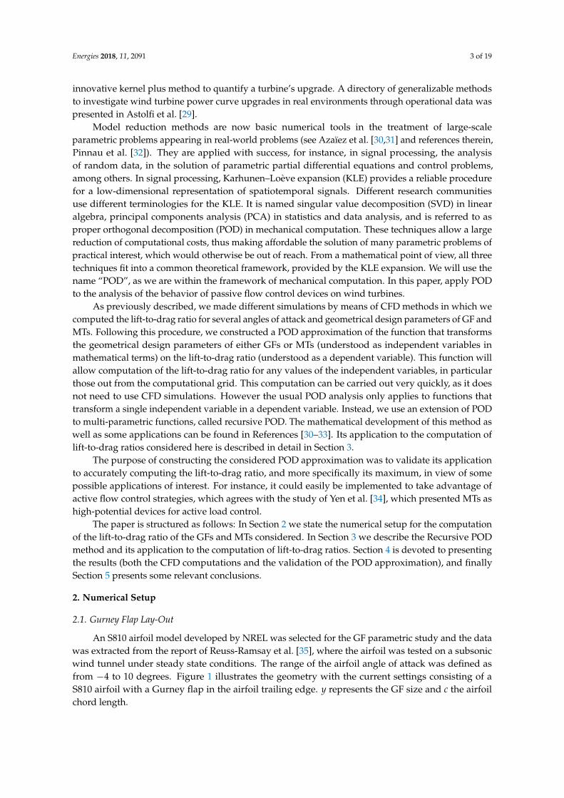
An S810 airfoil model developed by NREL was selected for the GF parametric study and the datawas extracted from the report of Reuss-Ramsay et al. [35], where the airfoil was tested on a subsonicwind tunnel under steady state conditions. The range of the airfoil angle of attack was defined asfrom −4 to 10 degrees. Figure 1 illustrates the geometry with the current settings consisting of aS810 airfoil with a Gurney flap in the airfoil trailing edge. y represents the GF size and c the airfoilchord length.

Energies 2018, 11, 2091 4 of 19Energies 2016, 9, x FOR PEER REVIEW 4 of 18

Figure 1. S810 National Renewable Energy Laboratory (NREL) aerodynamic airfoil and Gurney flap

(GF) dimension.

Dimension y represents the height of the GF in percentage of c. Twelve cases were analyzed

depending on the distance measured respective to the airfoil chord length (see Table 1).

Table 1. Case names and GF dimensions.

Id Case Name y (% of c)

0 S810 no GF

1 S810GF025 0.25

2 S810GF050 0.50

3 S810GF075 0.75

4 S810GF100 1.00

5 S810GF125 1.25

6 S810GF150 1.50

7 S810GF175 1.75

8 S810GF200 2.00

9 S810GF225 2.25

10 S810GF250 2.50

11 S810GF275 2.75

12 S810GF300 3.00

The numerical solution was performed applying Reynolds Averaged Navier–Stokes (RANS)

equations for steady state flow in the open source CFD code OpenFOAM (Version 2.4.0, The

OpenFOAM Foundation Ltd., London, UK) [36]. The SIMPLE algorithm has been used for the

coupling of pressure–velocity and a second-order linear-upwind scheme for the discretization of the

convective terms. The k- Shear Stress Transport (SST) turbulence model of Menter [37] has been

used for these computations due to its higher performance in separated flows, as reported by Kral

[38] and Gatski [39]. This model is a blend of the well known Wilcox’s k-ω model and the k-ε model.

RANS based simulations with the SST turbulence model for different configurations are presented in

the study of Mayda et al. [40] for airfoil applications. The Reynold number is Re = 106 based on the

airfoil chord length of c = 1 m. The grid of the computations consists of 155,000 structured cells, with

the first cell height ∆z/c of 1.45 × 10−6, where c is the airfoil chord length. The stretching factor in the

chord-wise and normal directions is made by double-sided tanh functions based on Thompson et al.

[41] and Vinokur [42]. The numerical domain was determined to have a wall y + less than 1 over the

surface of the airfoil. The domain was designed with a radius of 32 times the airfoil chord length,

according to the recommendations of Sørensen et al. [43]. The dimensions of the computational

domain normalized with the airfoil chord length are shown in Figure 2.

Figure 1. S810 National Renewable Energy Laboratory (NREL) aerodynamic airfoil and Gurney flap(GF) dimension.

Dimension y represents the height of the GF in percentage of c. Twelve cases were analyzeddepending on the distance measured respective to the airfoil chord length (see Table 1).

Table 1. Case names and GF dimensions.

Id Case Name y (% of c)

0 S810 no GF1 S810GF025 0.252 S810GF050 0.503 S810GF075 0.754 S810GF100 1.005 S810GF125 1.256 S810GF150 1.507 S810GF175 1.758 S810GF200 2.009 S810GF225 2.2510 S810GF250 2.5011 S810GF275 2.7512 S810GF300 3.00

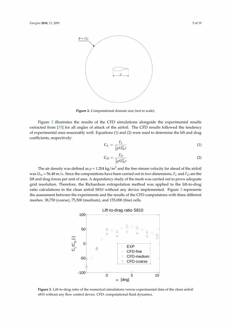
The numerical solution was performed applying Reynolds Averaged Navier–Stokes (RANS)equations for steady state flow in the open source CFD code OpenFOAM (Version 2.4.0,The OpenFOAM Foundation Ltd., London, UK) [36]. The SIMPLE algorithm has been used forthe coupling of pressure–velocity and a second-order linear-upwind scheme for the discretization ofthe convective terms. The k-ω Shear Stress Transport (SST) turbulence model of Menter [37] has beenused for these computations due to its higher performance in separated flows, as reported by Kral [38]and Gatski [39]. This model is a blend of the well known Wilcox’s k-ωmodel and the k-εmodel. RANSbased simulations with the SST turbulence model for different configurations are presented in the studyof Mayda et al. [40] for airfoil applications. The Reynold number is Re = 106 based on the airfoil chordlength of c = 1 m. The grid of the computations consists of 155,000 structured cells, with the first cellheight ∆z/c of 1.45 × 10−6, where c is the airfoil chord length. The stretching factor in the chord-wiseand normal directions is made by double-sided tanh functions based on Thompson et al. [41] andVinokur [42]. The numerical domain was determined to have a wall y + less than 1 over the surface ofthe airfoil. The domain was designed with a radius of 32 times the airfoil chord length, according tothe recommendations of Sørensen et al. [43]. The dimensions of the computational domain normalizedwith the airfoil chord length are shown in Figure 2.

Energies 2018, 11, 2091 5 of 19Energies 2016, 9, x FOR PEER REVIEW 5 of 18

Figure 2. Computational domain size (not to scale).

Figure 3 illustrates the results of the CFD simulations alongside the experimental results

extracted from [35] for all angles of attack of the airfoil. The CFD results followed the tendency of

experimental ones reasonably well. Equations (1) and (2) were used to determine the lift and drag

coefficients, respectively:

CL =𝐹𝐿

12

𝜌𝑈∞2 𝑐

(1)

CD =𝐹𝐷

12

𝜌𝑈∞2 𝑐

(2)

The air density was defined as ρ = 1.204 kg/m3 and the free stream velocity far ahead of the airfoil

was U∞ = 56.48 m/s. Since the computations have been carried out in two dimensions, FL and FD are

the lift and drag forces per unit of area. A dependency study of the mesh was carried out to prove

adequate grid resolution. Therefore, the Richardson extrapolation method was applied to the lift-to-

drag ratio calculations in the clean airfoil S810 without any device implemented. Figure 3 represents

the assessment between the experiments and the results of the CFD computatons with three different

meshes: 38,750 (coarse), 75,500 (medium), and 155,000 (fine) cells.

Figure 3. Lift-to-drag ratio of the numerical simulations versus experimental data of the clean airfoil

s810 without any flow control device. CFD: computational fluid dynamics.

0 5 10-100

-50

0

50

100

[deg]

CL/C

D [-]

Lift-to-drag ratio S810

EXP

CFD-fine

CFD-medium

CFD-coarse

Figure 2. Computational domain size (not to scale).

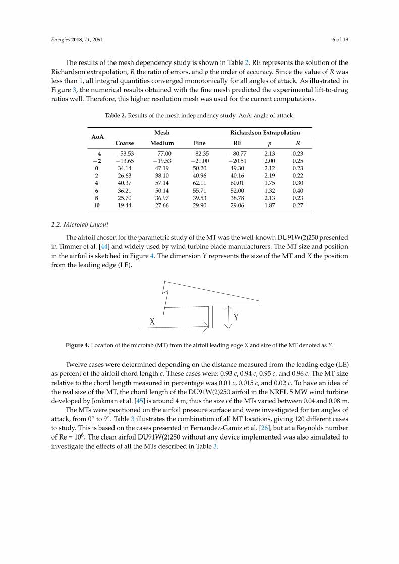
Figure 3 illustrates the results of the CFD simulations alongside the experimental resultsextracted from [35] for all angles of attack of the airfoil. The CFD results followed the tendencyof experimental ones reasonably well. Equations (1) and (2) were used to determine the lift and dragcoefficients, respectively:

CL =FL

12 ρU2

∞c(1)

CD =FD

12 ρU2

∞c(2)

The air density was defined as ρ = 1.204 kg/m3 and the free stream velocity far ahead of the airfoilwas U∞ = 56.48 m/s. Since the computations have been carried out in two dimensions, FL and FD are thelift and drag forces per unit of area. A dependency study of the mesh was carried out to prove adequategrid resolution. Therefore, the Richardson extrapolation method was applied to the lift-to-dragratio calculations in the clean airfoil S810 without any device implemented. Figure 3 representsthe assessment between the experiments and the results of the CFD computatons with three differentmeshes: 38,750 (coarse), 75,500 (medium), and 155,000 (fine) cells.

Energies 2016, 9, x FOR PEER REVIEW 5 of 18

Figure 2. Computational domain size (not to scale).

Figure 3 illustrates the results of the CFD simulations alongside the experimental results

extracted from [35] for all angles of attack of the airfoil. The CFD results followed the tendency of

experimental ones reasonably well. Equations (1) and (2) were used to determine the lift and drag

coefficients, respectively:

CL =𝐹𝐿

12

𝜌𝑈∞2 𝑐

(1)

CD =𝐹𝐷

12

𝜌𝑈∞2 𝑐

(2)

The air density was defined as ρ = 1.204 kg/m3 and the free stream velocity far ahead of the airfoil

was U∞ = 56.48 m/s. Since the computations have been carried out in two dimensions, FL and FD are

the lift and drag forces per unit of area. A dependency study of the mesh was carried out to prove

adequate grid resolution. Therefore, the Richardson extrapolation method was applied to the lift-to-

drag ratio calculations in the clean airfoil S810 without any device implemented. Figure 3 represents

the assessment between the experiments and the results of the CFD computatons with three different

meshes: 38,750 (coarse), 75,500 (medium), and 155,000 (fine) cells.

Figure 3. Lift-to-drag ratio of the numerical simulations versus experimental data of the clean airfoil

s810 without any flow control device. CFD: computational fluid dynamics.

0 5 10-100

-50

0

50

100

[deg]

CL/C

D [-]

Lift-to-drag ratio S810

EXP

CFD-fine

CFD-medium

CFD-coarse

Figure 3. Lift-to-drag ratio of the numerical simulations versus experimental data of the clean airfoils810 without any flow control device. CFD: computational fluid dynamics.

Energies 2018, 11, 2091 6 of 19

The results of the mesh dependency study is shown in Table 2. RE represents the solution of theRichardson extrapolation, R the ratio of errors, and p the order of accuracy. Since the value of R wasless than 1, all integral quantities converged monotonically for all angles of attack. As illustrated inFigure 3, the numerical results obtained with the fine mesh predicted the experimental lift-to-dragratios well. Therefore, this higher resolution mesh was used for the current computations.

Table 2. Results of the mesh independency study. AoA: angle of attack.

AoAMesh Richardson Extrapolation

Coarse Medium Fine RE p R

−4 −53.53 −77.00 −82.35 −80.77 2.13 0.23−2 −13.65 −19.53 −21.00 −20.51 2.00 0.250 34.14 47.19 50.20 49.30 2.12 0.232 26.63 38.10 40.96 40.16 2.19 0.224 40.37 57.14 62.11 60.01 1.75 0.306 36.21 50.14 55.71 52.00 1.32 0.408 25.70 36.97 39.53 38.78 2.13 0.23

10 19.44 27.66 29.90 29.06 1.87 0.27

2.2. Microtab Layout

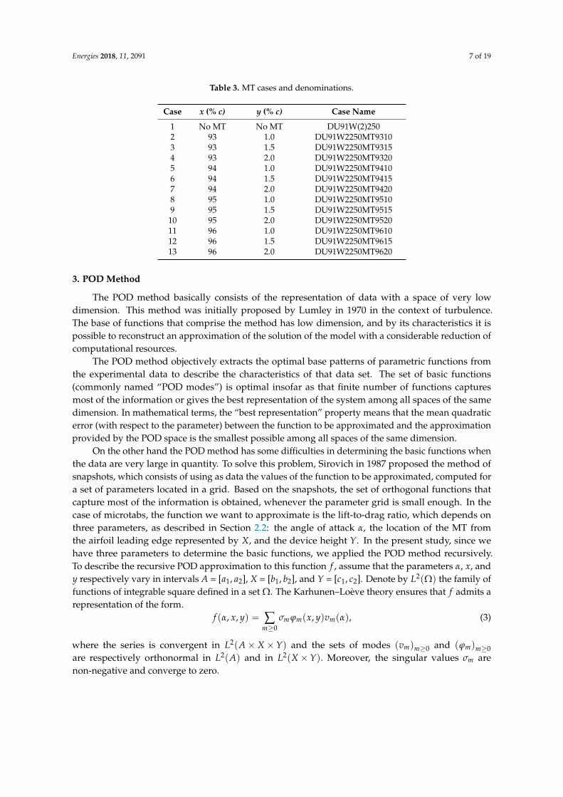
The airfoil chosen for the parametric study of the MT was the well-known DU91W(2)250 presentedin Timmer et al. [44] and widely used by wind turbine blade manufacturers. The MT size and positionin the airfoil is sketched in Figure 4. The dimension Y represents the size of the MT and X the positionfrom the leading edge (LE).

Energies 2016, 9, x FOR PEER REVIEW 6 of 18

The results of the mesh dependency study is shown in Table 2. RE represents the solution of the

Richardson extrapolation, R the ratio of errors, and p the order of accuracy. Since the value of R was

less than 1, all integral quantities converged monotonically for all angles of attack. As illustrated in

Figure 3, the numerical results obtained with the fine mesh predicted the experimental lift-to-drag

ratios well. Therefore, this higher resolution mesh was used for the current computations.

Table 2. Results of the mesh independency study. AoA: angle of attack.

AoA Mesh Richardson Extrapolation

Coarse Medium Fine RE p R

−4 −53.53 −77.00 −82.35 −80.77 2.13 0.23

−2 −13.65 −19.53 −21.00 −20.51 2.00 0.25

0 34.14 47.19 50.20 49.30 2.12 0.23

2 26.63 38.10 40.96 40.16 2.19 0.22

4 40.37 57.14 62.11 60.01 1.75 0.30

6 36.21 50.14 55.71 52.00 1.32 0.40

8 25.70 36.97 39.53 38.78 2.13 0.23

10 19.44 27.66 29.90 29.06 1.87 0.27

2.2. Microtab Layout

The airfoil chosen for the parametric study of the MT was the well-known DU91W(2)250

presented in Timmer et al. [44] and widely used by wind turbine blade manufacturers. The MT size

and position in the airfoil is sketched in Figure 4. The dimension Y represents the size of the MT and

X the position from the leading edge (LE).

Figure 4. Location of the microtab (MT) from the airfoil leading edge X and size of the MT denoted

as Y.

Twelve cases were determined depending on the distance measured from the leading edge (LE)

as percent of the airfoil chord length c. These cases were: 0.93 c, 0.94 c, 0.95 c, and 0.96 c. The MT size

relative to the chord length measured in percentage was 0.01 c, 0.015 c, and 0.02 c. To have an idea of

the real size of the MT, the chord length of the DU91W(2)250 airfoil in the NREL 5 MW wind turbine

developed by Jonkman et al. [45] is around 4 m, thus the size of the MTs varied between 0.04 and 0.08

m.

The MTs were positioned on the airfoil pressure surface and were investigated for ten angles of

attack, from 0° to 9°. Table 3 illustrates the combination of all MT locations, giving 120 different cases

to study. This is based on the cases presented in Fernandez-Gamiz et al. [26], but at a Reynolds

number of Re = 106. The clean airfoil DU91W(2)250 without any device implemented was also

simulated to investigate the effects of all the MTs described in Table 3.

Table 3. MT cases and denominations.

Case x (% c) y (% c) Case Name

1 No MT No MT DU91W(2)250

2 93 1.0 DU91W2250MT9310

3 93 1.5 DU91W2250MT9315

4 93 2.0 DU91W2250MT9320

YX

Figure 4. Location of the microtab (MT) from the airfoil leading edge X and size of the MT denoted as Y.

Twelve cases were determined depending on the distance measured from the leading edge (LE)as percent of the airfoil chord length c. These cases were: 0.93 c, 0.94 c, 0.95 c, and 0.96 c. The MT sizerelative to the chord length measured in percentage was 0.01 c, 0.015 c, and 0.02 c. To have an idea ofthe real size of the MT, the chord length of the DU91W(2)250 airfoil in the NREL 5 MW wind turbinedeveloped by Jonkman et al. [45] is around 4 m, thus the size of the MTs varied between 0.04 and 0.08 m.

The MTs were positioned on the airfoil pressure surface and were investigated for ten angles ofattack, from 0 to 9. Table 3 illustrates the combination of all MT locations, giving 120 different casesto study. This is based on the cases presented in Fernandez-Gamiz et al. [26], but at a Reynolds numberof Re = 106. The clean airfoil DU91W(2)250 without any device implemented was also simulated toinvestigate the effects of all the MTs described in Table 3.

Energies 2018, 11, 2091 7 of 19

Table 3. MT cases and denominations.

Case x (% c) y (% c) Case Name

1 No MT No MT DU91W(2)2502 93 1.0 DU91W2250MT93103 93 1.5 DU91W2250MT93154 93 2.0 DU91W2250MT93205 94 1.0 DU91W2250MT94106 94 1.5 DU91W2250MT94157 94 2.0 DU91W2250MT94208 95 1.0 DU91W2250MT95109 95 1.5 DU91W2250MT9515

10 95 2.0 DU91W2250MT952011 96 1.0 DU91W2250MT961012 96 1.5 DU91W2250MT961513 96 2.0 DU91W2250MT9620

3. POD Method

The POD method basically consists of the representation of data with a space of very lowdimension. This method was initially proposed by Lumley in 1970 in the context of turbulence.The base of functions that comprise the method has low dimension, and by its characteristics it ispossible to reconstruct an approximation of the solution of the model with a considerable reduction ofcomputational resources.

The POD method objectively extracts the optimal base patterns of parametric functions fromthe experimental data to describe the characteristics of that data set. The set of basic functions(commonly named “POD modes”) is optimal insofar as that finite number of functions capturesmost of the information or gives the best representation of the system among all spaces of the samedimension. In mathematical terms, the “best representation” property means that the mean quadraticerror (with respect to the parameter) between the function to be approximated and the approximationprovided by the POD space is the smallest possible among all spaces of the same dimension.

On the other hand the POD method has some difficulties in determining the basic functions whenthe data are very large in quantity. To solve this problem, Sirovich in 1987 proposed the method ofsnapshots, which consists of using as data the values of the function to be approximated, computed fora set of parameters located in a grid. Based on the snapshots, the set of orthogonal functions thatcapture most of the information is obtained, whenever the parameter grid is small enough. In thecase of microtabs, the function we want to approximate is the lift-to-drag ratio, which depends onthree parameters, as described in Section 2.2: the angle of attack α, the location of the MT fromthe airfoil leading edge represented by X, and the device height Y. In the present study, since wehave three parameters to determine the basic functions, we applied the POD method recursively.To describe the recursive POD approximation to this function f , assume that the parameters α, x, andy respectively vary in intervals A = [a1, a2], X = [b1, b2], and Y = [c1, c2]. Denote by L2(Ω) the family offunctions of integrable square defined in a set Ω. The Karhunen–Loève theory ensures that f admits arepresentation of the form.

f (α, x, y) = ∑m≥0

σm ϕm(x, y)vm(α), (3)

where the series is convergent in L2(A × X × Y) and the sets of modes (vm)m≥0 and (ϕm)m≥0are respectively orthonormal in L2(A) and in L2(X × Y). Moreover, the singular values σm arenon-negative and converge to zero.

Energies 2018, 11, 2091 8 of 19

We next applied the POD expansion to each mode ϕm(x, y). There are two sets of modes(u(m)

k

)k≥0

and(

w(m)k

)k≥0

which are respectively orthonormal in L2(X) and L2(Y), such that ϕm

admits the representation:ϕm(x, y) = ∑

k≥0σ(m)k u(m)

k (x)w(m)k (y), (4)

where the expansion is convergent in L2(X × Y). Additionally, the singular values(

σ(m)k

)k≥0

are

non-negative and decrease to zero. Then, the function f admits the expansion:

f (α, x, y) = ∑m≥0

∑k≥0

σmσ(m)k vm(α)u

(m)k (x)w(m)

k (y), (5)

where the sum is convergent in L2(A × X × Y). The feasible recursive POD approximation of thefunction f consists of truncating the series (3) and (5) to a finite number of summands (e.g., M andK). Further, as the function f can be computed only for some values of α : α1, . . . , αN , x = x1, . . . , xP,and y = y1, . . .,yQ, the recursive POD in principle provides an approximation of f at these values:

f(αi, xj, yl

)=

M

∑m=0

K

∑k=0

σmσ(m)k vm(αi)u

(m)k(xj)w(m)

k (yl). (6)

Then, a fast 1D interpolation procedure (e.g., by spline functions) is used to compute f (α, x, y) fordifferent values of (α, x, y) in A × X × Y. The source of errors in the recursive POD approximation isnot only the truncation of series (6), but also this interpolation procedure. Then, the interpolation gridsize should be small enough to ensure good error levels. Note that the interpolation grid is actuallythe parameter grid for which the values f

(αi, xj, yl

)are computed, and a decrease in grid size leads to

a larger number of CFD computations.The computation of the POD expansion for bi-variate functions (e.g., for function ϕm at

regularly spaced grid nodes x = x1, . . . , xP and y = y1, . . .,yQ) is as follows: The vectors

Uk =[u(m)

k (x1), . . . , u(m)k (xP)

]and Wk =

[w(m)

k (y1), . . . , w(m)k(yQ)]

respectively are theK ≤ minP,Q first right and left eigenvectors of the singular value decomposition of the matrix:

X(m) =

ϕ(m)(x1, y1) · · · ϕ(m)(xP, y1)...

. . ....

ϕ(m)(x1, yQ

)· · · ϕ(m)

(xP, yQ

)

while the coefficients σ(m)k , k = 1, . . . , K are the corresponding singular values.

Figure 5 illustrates the error that is committed in the method for different norms to approximatea smooth function of two variables, reported in Azaïez et al. [31]. On the x-axis we have the totalnumber of modes M, and on the y-axis we have the error that is committed in logarithmic coordinates.We can observe that very few modes provided an excellent approximation of our function. The resultspresented in Section 4 were achieved with seven modes.

Energies 2018, 11, 2091 9 of 19

Energies 2016, 9, x FOR PEER REVIEW 8 of 18

𝑓(𝛼, 𝑥, 𝑦) = ∑ ∑ 𝜎𝑚𝜎𝑘(𝑚)

𝑘≥0𝑚≥0

𝑣𝑚(𝛼)𝑢𝑘(𝑚)(𝑥)𝑤𝑘

(𝑚)(𝑦), (5)

where the sum is convergent in 𝐿2(𝐴 × 𝑋 × 𝑌). The feasible recursive POD approximation of the

function 𝑓 consists of truncating the series (3) and (5) to a finite number of summands (e.g., M and

K). Further, as the function 𝑓 can be computed only for some values of 𝛼: 𝛼1, … , 𝛼𝑁 , 𝑥 = 𝑥1, … , 𝑥𝑃,

and 𝑦 = 𝑦1, …,𝑦𝑄 , the recursive POD in principle provides an approximation of 𝑓 at these values:

𝑓(𝛼𝑖 , 𝑥𝑗 , 𝑦𝑙) = ∑ ∑ 𝜎𝑚𝜎𝑘(𝑚)

𝐾

𝑘=0

𝑀

𝑚=0

𝑣𝑚(𝛼𝑖)𝑢𝑘(𝑚)

(𝑥𝑗)𝑤𝑘(𝑚)(𝑦𝑙). (6)

Then, a fast 1D interpolation procedure (e.g., by spline functions) is used to compute 𝑓(𝛼, 𝑥, 𝑦)

for different values of (𝛼, 𝑥, 𝑦) in 𝐴 × 𝑋 × 𝑌 . The source of errors in the recursive POD

approximation is not only the truncation of series (6), but also this interpolation procedure. Then, the

interpolation grid size should be small enough to ensure good error levels. Note that the interpolation

grid is actually the parameter grid for which the values 𝑓(𝛼𝑖 , 𝑥𝑗 , 𝑦𝑙) are computed, and a decrease in

grid size leads to a larger number of CFD computations.

The computation of the POD expansion for bi-variate functions (e.g., for function 𝜑𝑚 at

regularly spaced grid nodes 𝑥 = 𝑥1, … , 𝑥𝑃 and 𝑦 = 𝑦1, … , 𝑦𝑄 ) is as follows: The vectors 𝑈𝑘 =

[𝑢𝑘(𝑚)(𝑥1), … , 𝑢𝑘

(𝑚)(𝑥𝑃)] and 𝑊𝑘 = [𝑤𝑘(𝑚)(𝑦1), … , 𝑤𝑘

(𝑚)(𝑦𝑄)] respectively are the K ≤ minP,Q first

right and left eigenvectors of the singular value decomposition of the matrix:

𝑋(𝑚) = (𝜑(𝑚)(𝑥1, 𝑦1) ⋯ 𝜑(𝑚)(𝑥𝑃 , 𝑦1)

⋮ ⋱ ⋮𝜑(𝑚)(𝑥1, 𝑦𝑄) ⋯ 𝜑(𝑚)(𝑥𝑃 , 𝑦𝑄)

)

while the coefficients 𝜎𝑘(𝑚)

, 𝑘 = 1, … , 𝐾 are the corresponding singular values.

Figure 5 illustrates the error that is committed in the method for different norms to approximate

a smooth function of two variables, reported in Azaïez et al. [31]. On the x-axis we have the total

number of modes M, and on the y-axis we have the error that is committed in logarithmic coordinates.

We can observe that very few modes provided an excellent approximation of our function. The results

presented in Section 4 were achieved with seven modes.

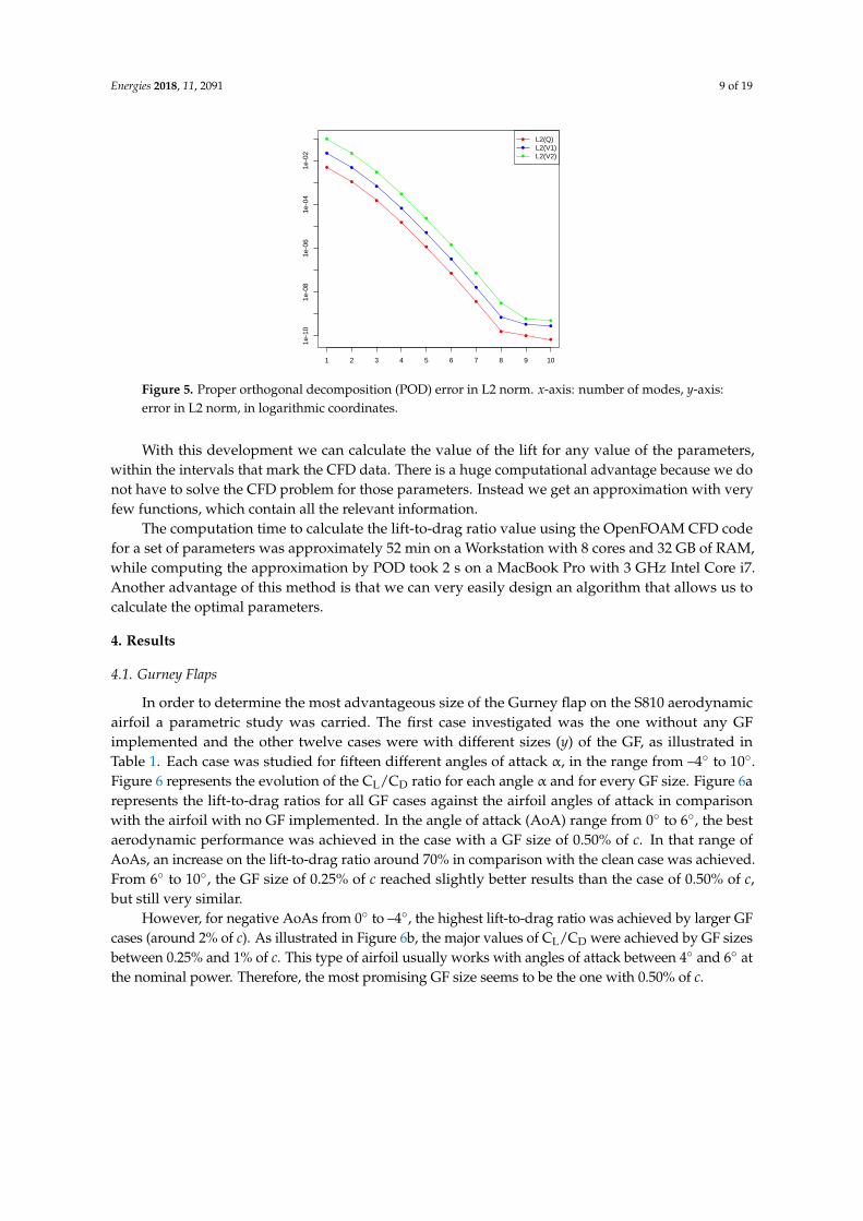
Figure 5. Proper orthogonal decomposition (POD) error in L2 norm. x-axis: number of modes, y-axis:

error in L2 norm, in logarithmic coordinates.

With this development we can calculate the value of the lift for any value of the parameters,

within the intervals that mark the CFD data. There is a huge computational advantage because we

do not have to solve the CFD problem for those parameters. Instead we get an approximation with

very few functions, which contain all the relevant information.

1 2 3 4 5 6 7 8 9 10

1e

-10

1e

-08

1e

-06

1e

-04

1e

-02

L2(Q)

L2(V1)

L2(V2)

Figure 5. Proper orthogonal decomposition (POD) error in L2 norm. x-axis: number of modes, y-axis:error in L2 norm, in logarithmic coordinates.

With this development we can calculate the value of the lift for any value of the parameters,within the intervals that mark the CFD data. There is a huge computational advantage because we donot have to solve the CFD problem for those parameters. Instead we get an approximation with veryfew functions, which contain all the relevant information.

The computation time to calculate the lift-to-drag ratio value using the OpenFOAM CFD codefor a set of parameters was approximately 52 min on a Workstation with 8 cores and 32 GB of RAM,while computing the approximation by POD took 2 s on a MacBook Pro with 3 GHz Intel Core i7.Another advantage of this method is that we can very easily design an algorithm that allows us tocalculate the optimal parameters.

4. Results

4.1. Gurney Flaps

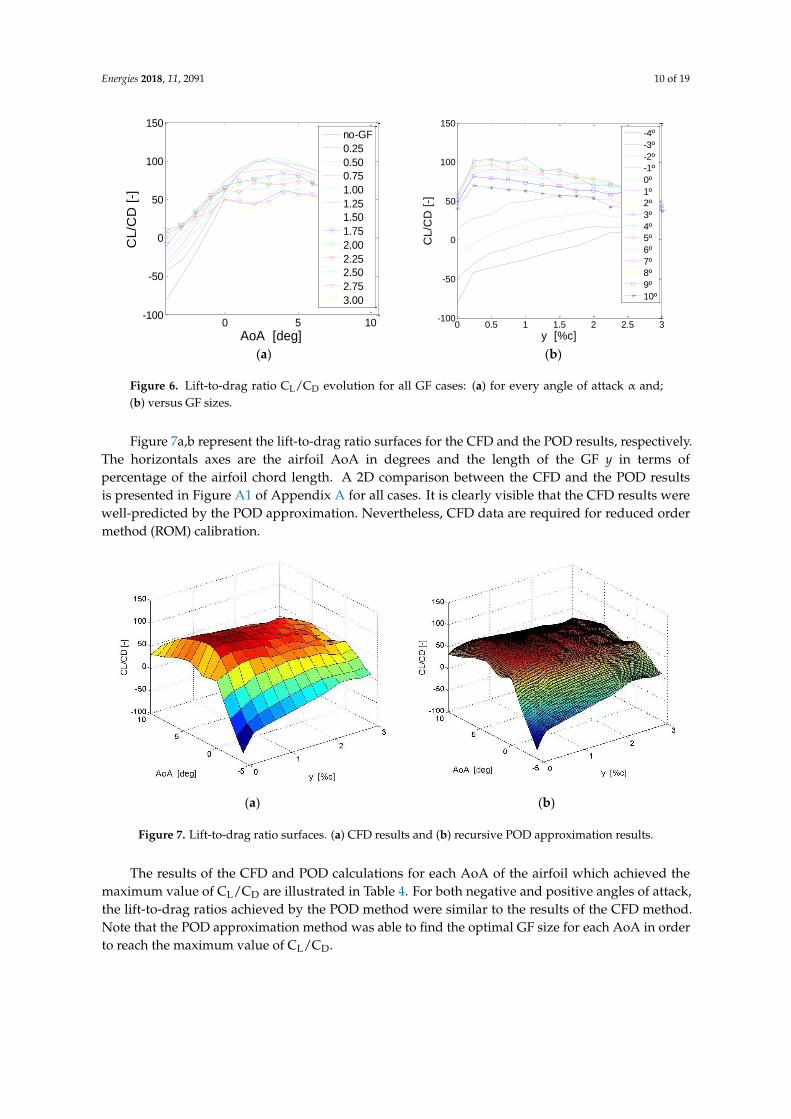
In order to determine the most advantageous size of the Gurney flap on the S810 aerodynamicairfoil a parametric study was carried. The first case investigated was the one without any GFimplemented and the other twelve cases were with different sizes (y) of the GF, as illustrated inTable 1. Each case was studied for fifteen different angles of attack α, in the range from –4 to 10.Figure 6 represents the evolution of the CL/CD ratio for each angle α and for every GF size. Figure 6arepresents the lift-to-drag ratios for all GF cases against the airfoil angles of attack in comparisonwith the airfoil with no GF implemented. In the angle of attack (AoA) range from 0 to 6, the bestaerodynamic performance was achieved in the case with a GF size of 0.50% of c. In that range ofAoAs, an increase on the lift-to-drag ratio around 70% in comparison with the clean case was achieved.From 6 to 10, the GF size of 0.25% of c reached slightly better results than the case of 0.50% of c,but still very similar.

However, for negative AoAs from 0 to –4, the highest lift-to-drag ratio was achieved by larger GFcases (around 2% of c). As illustrated in Figure 6b, the major values of CL/CD were achieved by GF sizesbetween 0.25% and 1% of c. This type of airfoil usually works with angles of attack between 4 and 6 atthe nominal power. Therefore, the most promising GF size seems to be the one with 0.50% of c.

Energies 2018, 11, 2091 10 of 19

Energies 2016, 9, x FOR PEER REVIEW 9 of 18

The computation time to calculate the lift-to-drag ratio value using the OpenFOAM CFD code

for a set of parameters was approximately 52 min on a Workstation with 8 cores and 32 GB of RAM,

while computing the approximation by POD took 2 s on a MacBook Pro with 3 GHz Intel Core i7.

Another advantage of this method is that we can very easily design an algorithm that allows us to

calculate the optimal parameters.

4. Results

4.1. Gurney Flaps

In order to determine the most advantageous size of the Gurney flap on the S810 aerodynamic

airfoil a parametric study was carried. The first case investigated was the one without any GF

implemented and the other twelve cases were with different sizes (y) of the GF, as illustrated in Table

1. Each case was studied for fifteen different angles of attack α, in the range from –4° to 10°. Figure 6

represents the evolution of the CL/CD ratio for each angle α and for every GF size. Figure 6a represents

the lift-to-drag ratios for all GF cases against the airfoil angles of attack in comparison with the airfoil

with no GF implemented. In the angle of attack (AoA) range from 0° to 6°, the best aerodynamic

performance was achieved in the case with a GF size of 0.50% of c. In that range of AoAs, an increase

on the lift-to-drag ratio around 70% in comparison with the clean case was achieved. From 6° to 10°,

the GF size of 0.25% of c reached slightly better results than the case of 0.50% of c, but still very similar.

However, for negative AoAs from 0° to –4°, the highest lift-to-drag ratio was achieved by larger

GF cases (around 2% of c). As illustrated in Figure 6b, the major values of CL/CD were achieved by GF

sizes between 0.25% and 1% of c. This type of airfoil usually works with angles of attack between 4°

and 6° at the nominal power. Therefore, the most promising GF size seems to be the one with 0.50%

of c.

(a) (b)

Figure 6. Lift-to-drag ratio CL/CD evolution for all GF cases: (a) for every angle of attack α and; (b)

versus GF sizes.

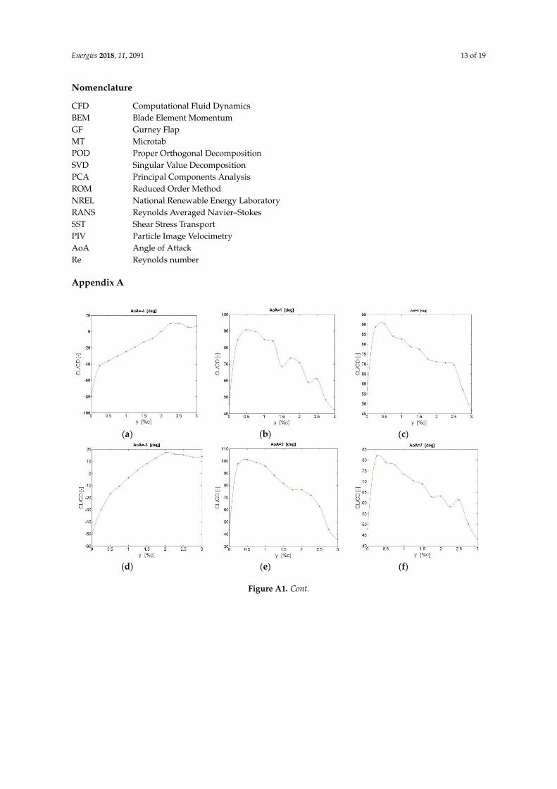
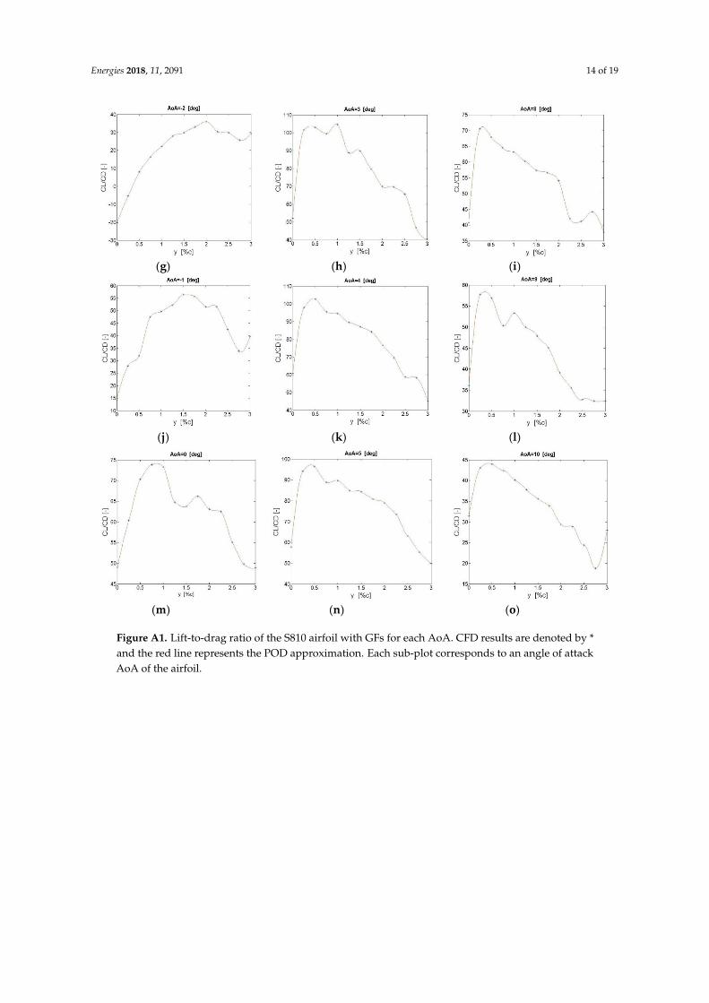
Figures 7a and 7b represent the lift-to-drag ratio surfaces for the CFD and the POD results,

respectively. The horizontals axes are the airfoil AoA in degrees and the length of the GF y in terms

of percentage of the airfoil chord length. A 2D comparison between the CFD and the POD results is

presented in Figure A1 of Appendix A for all cases. It is clearly visible that the CFD results were well-

predicted by the POD approximation. Nevertheless, CFD data are required for reduced order method

(ROM) calibration.

0 5 10-100

-50

0

50

100

150

AoA [deg]

CL/C

D [

-]

no-GF

0.25

0.50

0.75

1.00

1.25

1.50

1.75

2.00

2.25

2.50

2.75

3.00

0 0.5 1 1.5 2 2.5 3-100

-50

0

50

100

150

y [%c]

CL/C

D [

-]

-4º

-3º

-2º

-1º

0º

1º

2º

3º

4º

5º

6º

7º

8º

9º

10º

Figure 6. Lift-to-drag ratio CL/CD evolution for all GF cases: (a) for every angle of attack α and;(b) versus GF sizes.

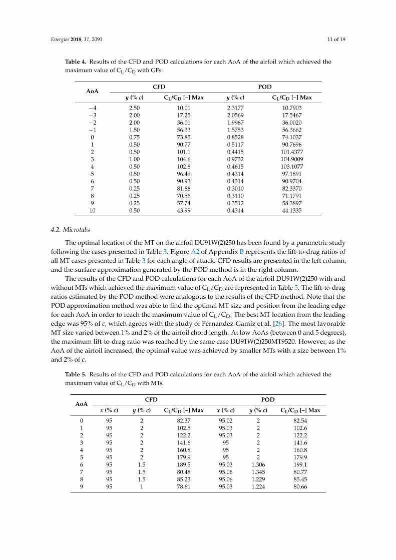
Figure 7a,b represent the lift-to-drag ratio surfaces for the CFD and the POD results, respectively.The horizontals axes are the airfoil AoA in degrees and the length of the GF y in terms ofpercentage of the airfoil chord length. A 2D comparison between the CFD and the POD resultsis presented in Figure A1 of Appendix A for all cases. It is clearly visible that the CFD results werewell-predicted by the POD approximation. Nevertheless, CFD data are required for reduced ordermethod (ROM) calibration.Energies 2016, 9, x FOR PEER REVIEW 10 of 18

(a) (b)

Figure 7. Lift-to-drag ratio surfaces. (a) CFD results and (b) recursive POD approximation results.

The results of the CFD and POD calculations for each AoA of the airfoil which achieved the

maximum value of CL/CD are illustrated in Table 4. For both negative and positive angles of attack,

the lift-to-drag ratios achieved by the POD method were similar to the results of the CFD method.

Note that the POD approximation method was able to find the optimal GF size for each AoA in order

to reach the maximum value of CL/CD.

Table 4. Results of the CFD and POD calculations for each AoA of the airfoil which achieved the

maximum value of CL/CD with GFs.

AoA CFD POD

y (% c) CL/CD [–] Max y (% c) CL/CD [–] Max

−4 2.50 10.01 2.3177 10.7903

−3 2.00 17.25 2.0569 17.5467

−2 2.00 36.01 1.9967 36.0020

−1 1.50 56.33 1.5753 56.3662

0 0.75 73.85 0.8528 74.1037

1 0.50 90.77 0.5117 90.7696

2 0.50 101.1 0.4415 101.4377

3 1.00 104.6 0.9732 104.9009

4 0.50 102.8 0.4615 103.1077

5 0.50 96.49 0.4314 97.1891

6 0.50 90.93 0.4314 90.9704

7 0.25 81.88 0.3010 82.3370

8 0.25 70.56 0.3110 71.1791

9 0.25 57.74 0.3512 58.3897

10 0.50 43.99 0.4314 44.1335

4.2. Microtabs

The optimal location of the MT on the airfoil DU91W(2)250 has been found by a parametric

study following the cases presented in Table 3. Figure B1 of Appendix B represents the lift-to-drag

ratios of all MT cases presented in Table 3 for each angle of attack. CFD results are presented in the

left column, and the surface approximation generated by the POD method is in the right column.

The results of the CFD and POD calculations for each AoA of the airfoil DU91W(2)250 with and

without MTs which achieved the maximum value of CL/CD are represented in Table 5. The lift-to-

drag ratios estimated by the POD method were analogous to the results of the CFD method. Note

Figure 7. Lift-to-drag ratio surfaces. (a) CFD results and (b) recursive POD approximation results.

The results of the CFD and POD calculations for each AoA of the airfoil which achieved themaximum value of CL/CD are illustrated in Table 4. For both negative and positive angles of attack,the lift-to-drag ratios achieved by the POD method were similar to the results of the CFD method.Note that the POD approximation method was able to find the optimal GF size for each AoA in orderto reach the maximum value of CL/CD.

Energies 2018, 11, 2091 11 of 19

Table 4. Results of the CFD and POD calculations for each AoA of the airfoil which achieved themaximum value of CL/CD with GFs.

AoACFD POD

y (% c) CL/CD [–] Max y (% c) CL/CD [–] Max

−4 2.50 10.01 2.3177 10.7903−3 2.00 17.25 2.0569 17.5467−2 2.00 36.01 1.9967 36.0020−1 1.50 56.33 1.5753 56.36620 0.75 73.85 0.8528 74.10371 0.50 90.77 0.5117 90.76962 0.50 101.1 0.4415 101.43773 1.00 104.6 0.9732 104.90094 0.50 102.8 0.4615 103.10775 0.50 96.49 0.4314 97.18916 0.50 90.93 0.4314 90.97047 0.25 81.88 0.3010 82.33708 0.25 70.56 0.3110 71.17919 0.25 57.74 0.3512 58.389710 0.50 43.99 0.4314 44.1335

4.2. Microtabs

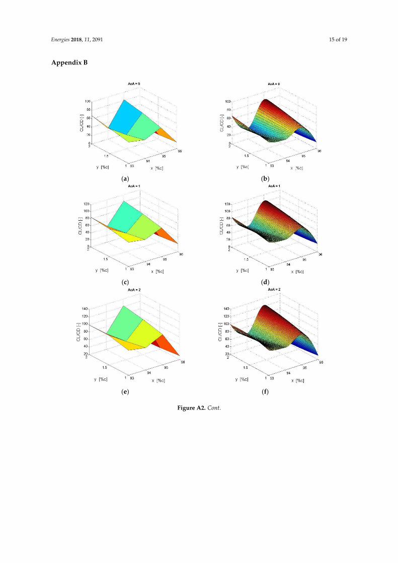
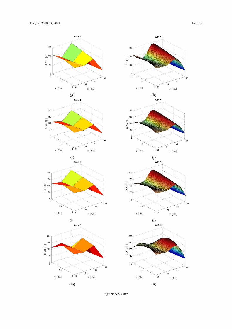
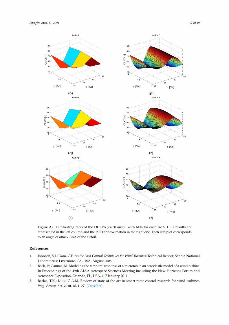
The optimal location of the MT on the airfoil DU91W(2)250 has been found by a parametric studyfollowing the cases presented in Table 3. Figure A2 of Appendix B represents the lift-to-drag ratios ofall MT cases presented in Table 3 for each angle of attack. CFD results are presented in the left column,and the surface approximation generated by the POD method is in the right column.

The results of the CFD and POD calculations for each AoA of the airfoil DU91W(2)250 with andwithout MTs which achieved the maximum value of CL/CD are represented in Table 5. The lift-to-dragratios estimated by the POD method were analogous to the results of the CFD method. Note that thePOD approximation method was able to find the optimal MT size and position from the leading edgefor each AoA in order to reach the maximum value of CL/CD. The best MT location from the leadingedge was 95% of c, which agrees with the study of Fernandez-Gamiz et al. [26]. The most favorableMT size varied between 1% and 2% of the airfoil chord length. At low AoAs (between 0 and 5 degrees),the maximum lift-to-drag ratio was reached by the same case DU91W(2)250MT9520. However, as theAoA of the airfoil increased, the optimal value was achieved by smaller MTs with a size between 1%and 2% of c.

Table 5. Results of the CFD and POD calculations for each AoA of the airfoil which achieved themaximum value of CL/CD with MTs.

AoACFD POD

x (% c) y (% c) CL/CD [–] Max x (% c) y (% c) CL/CD [–] Max

0 95 2 82.37 95.02 2 82.541 95 2 102.5 95.03 2 102.62 95 2 122.2 95.03 2 122.23 95 2 141.6 95 2 141.64 95 2 160.8 95 2 160.85 95 2 179.9 95 2 179.96 95 1.5 189.5 95.03 1.306 199.17 95 1.5 80.48 95.06 1.345 80.778 95 1.5 85.23 95.06 1.229 85.459 95 1 78.61 95.03 1.224 80.66

Energies 2018, 11, 2091 12 of 19

According to the BEM-based computations of Fernandez-Gamiz et al. [26] and the wind turbineretrofitting study carried by Astolfi et al. [46], it is expected that the increase in the lift-to-drag ratiodue to the implementation of passive flow control devices could lead to an increase in the wind turbineenergy production. As explained in the work of Fernandez-Gamiz et al. [21] in a 5 MW wind turbine,the improvement in the power production could be more significant at low and moderate windspeeds. Additionally, the recursive POD developed in the current study could be easily implementedin the control system of a wind turbine to take advantage of active flow control strategies, which is inconcordance with the study of Yen et al. [34], who presented MTs as devices with high potential foractive load control.

5. Conclusions

Firstly, an investigation for the design and analysis of a GF on a S810 airfoil and of a MT on aDU91(2)250 airfoil was carried out. Two-dimensional computational fluid dynamic simulations wereperformed on these commonly used airfoils on wind turbines, using RANS equations at Re = 106.The GF and MT design attributes resulting from the CFD computations allowed sizing of the passivedevices based on the airfoil aerodynamic performance. In both types of flow control devices, theresults showed an increase in the lift-to-drag ratio for all angles of attack considered in the currentwork. In the case of the GFs, with AoAs from 0 to 6 degrees, the highest lift-to-drag ratio was achievedby the airfoil with the GF size of 0.50% of c. An enhancement of the lift-to-drag ratio around 70% incomparison with the clean case was achieved in that range of AoAs. From 6 to 10, the GF size of0.25% of c achieved superior but similar results to the case of 0.50% of c. It was found that the best MTlocation was 95% of c measured from the airfoil leading edge, and the most favorable MT size variedbetween 1% and 2% of the chord length of the airfoil. Between 0 and 6 of airfoil AoA, the maximumlift-to-drag ratio was reached by the case DU91W(2)250MT9515. Nevertheless, as the AoA of the airfoilincreased beyond 6, the most advantageous value was achieved by a shorter MT size.

Secondly, from the data obtained by means of CFD simulations, a regular function using thereduced order method of POD was built. In both flow control cases (GFs and MTs), the recursive PODmethod was able to accurately reproduce the computational results. The developed POD recursivemethod consists of two stages—one offline, and another online. The offline step consists of constructingthe function that transforms the geometrical and physical parameters on the lift-to-drag ratio, startingfrom lift-to-drag ratio data obtained by CFD computations. In the online step, this function is used todirectly compute the lift and drag coefficients for any given set of geometrical and physical parameters,without needing any CFD computation. This leads to a method with very low computational cost thatis extraordinarily fast.

The results of the present work show that careful analysis of the GF size and MT height andlocation from the airfoil leading edge can yield effective devices for flow control in order to improvethe airfoil aerodynamic performance. In addition, the POD method was revealed as a powerful toolto predict the lift-to-drag values of these types of parametric studies. The main conclusion of thispaper is the validation of recursive POD approximation’s ability to accurately compute the maximumlift–drag ratio associated with a given GF or MT configuration, in view of further applications in activeflow control.

Author Contributions: Unai Fernandez-Gamiz prepared the case studies and performed the CFD simulations.Macarena Gomez-Mármol and Tomas Chacón Rebollo made the POD calculations. The manuscript was structuredand written by all authors.

Funding: The current research was partially supported by the Spanish Government with the Project:grant number: MTM2015-64577-C2-1-R.

Acknowledgments: The authors are very grateful to the Spanish Government Project MTM2015-64577-C2-1-R.

Conflicts of Interest: The authors declare no conflict of interest.

Energies 2018, 11, 2091 13 of 19

Nomenclature

CFD Computational Fluid DynamicsBEM Blade Element MomentumGF Gurney FlapMT MicrotabPOD Proper Orthogonal DecompositionSVD Singular Value DecompositionPCA Principal Components AnalysisROM Reduced Order MethodNREL National Renewable Energy LaboratoryRANS Reynolds Averaged Navier–StokesSST Shear Stress TransportPIV Particle Image VelocimetryAoA Angle of AttackRe Reynolds number

Appendix A

Energies 2016, 9, x FOR PEER REVIEW 13 of 18

Appendix A

(a) (b) (c)

(d) (e) (f)

(g) (h) (i)

(j) (k) (l)

Figure A1. Cont.

Energies 2018, 11, 2091 14 of 19

Energies 2016, 9, x FOR PEER REVIEW 13 of 18

Appendix A

(a) (b) (c)

(d) (e) (f)

(g) (h) (i)

(j) (k) (l)

Energies 2016, 9, x FOR PEER REVIEW 14 of 18

(m) (n) (o)

Figure A1. Lift-to-drag ratio of the S810 airfoil with GFs for each AoA. CFD results are denoted by *

and the red line represents the POD approximation. Each sub-plot corresponds to an angle of attack

AoA of the airfoil.

Appendix B

(a) (b)

(c) (d)

(e) (f)

Figure A1. Lift-to-drag ratio of the S810 airfoil with GFs for each AoA. CFD results are denoted by *and the red line represents the POD approximation. Each sub-plot corresponds to an angle of attackAoA of the airfoil.

Energies 2018, 11, 2091 15 of 19

Appendix B

Energies 2016, 9, x FOR PEER REVIEW 14 of 18

(m) (n) (o)

Figure A1. Lift-to-drag ratio of the S810 airfoil with GFs for each AoA. CFD results are denoted by *

and the red line represents the POD approximation. Each sub-plot corresponds to an angle of attack

AoA of the airfoil.

Appendix B

(a) (b)

(c) (d)

(e) (f)

Figure A2. Cont.

Energies 2018, 11, 2091 16 of 19Energies 2016, 9, x FOR PEER REVIEW 15 of 18

(g) (h)

(i) (j)

(k) (l)

(m) (n)

Figure A2. Cont.

Energies 2018, 11, 2091 17 of 19Energies 2016, 9, x FOR PEER REVIEW 16 of 18

(o) (p)

(q) (r)

(s) (t)

Figure B1. Lift-to-drag ratio of the DU91W(2)250 airfoil with MTs for each AoA. CFD results are

represented in the left column and the POD approximation in the right one. Each sub-plot

corresponds to an angle of attack AoA of the airfoil.

References

1. Johnson, S.J.; Dam, C.P. Active Load Control Techniques for Wind Turbines. Technical Report; Sandia National

Laboratories: Livermore, CA, USA, August 2008.

2. Baek, P.; Gaunaa, M. Modeling the temporal response of a microtab in an aeroelastic model of a wind

turbine. In Proceedings of the 49th AIAA Aerospace Sciences Meeting including the New Horizons Forum

and Aerospace Exposition, Orlando, FL, USA, 4–7 January 2011.

3. Barlas, T.K.; Kuik, G.A.M. Review of state of the art in smart rotor control research for wind turbines. Prog.

Aerosp. Sci. 2010, 46, 1–27, doi:10.1016/j.paerosci.2009.08.002.

4. Wood, R.M. A Discussion of Aerodynamic Control Effectors Concepts (ACEs) for Future Unmanned Air

Vehicles (UAVs). In Proceedings of the AIAA 1st Technical Conference and Workshop on Unmanned

Aerospace Vehicle, Systems, Technologies, and Operations, Portsmouth, VA, USA, 20–23 May 2002.

Figure A2. Lift-to-drag ratio of the DU91W(2)250 airfoil with MTs for each AoA. CFD results arerepresented in the left column and the POD approximation in the right one. Each sub-plot correspondsto an angle of attack AoA of the airfoil.

References

1. Johnson, S.J.; Dam, C.P. Active Load Control Techniques for Wind Turbines; Technical Report; Sandia NationalLaboratories: Livermore, CA, USA, August 2008.

2. Baek, P.; Gaunaa, M. Modeling the temporal response of a microtab in an aeroelastic model of a wind turbine.In Proceedings of the 49th AIAA Aerospace Sciences Meeting including the New Horizons Forum andAerospace Exposition, Orlando, FL, USA, 4–7 January 2011.

3. Barlas, T.K.; Kuik, G.A.M. Review of state of the art in smart rotor control research for wind turbines.Prog. Aerosp. Sci. 2010, 46, 1–27. [CrossRef]

Energies 2018, 11, 2091 18 of 19

4. Wood, R.M. A Discussion of Aerodynamic Control Effectors Concepts (ACEs) for Future Unmanned AirVehicles (UAVs). In Proceedings of the AIAA 1st Technical Conference and Workshop on UnmannedAerospace Vehicle, Systems, Technologies, and Operations, Portsmouth, VA, USA, 20–23 May 2002.

5. Aramendia, I.; Fernandez-Gamiz, U.; Ramos-Hernanz, J.; Sancho, J.; Lopez-Guede, J.; Zulueta, E.Flow Control Devices for Wind Turbines. In Energy Harvesting and Energy Efficiency: Technology, Methods,and Applications; Bizon, N., Mahdavi Tabatabaei, N., Blaabjerg, F., Kurt, E., Eds.; Springer: Berlin, Germany,2017; pp. 629–655.

6. Aramendia-Iradi, I.; Fernandez-Gamiz, U.; Sancho-Saiz, J.; Zulueta-Guerrero, E. State of the art of active andpassive flow control devices for wind turbines. Dyna 2016, 91, 512–516. [CrossRef]

7. Johnson, S.J.; Baker, J.P.; van Dam, C.P.; Berg, D. An overview of active load control techniques for windturbines with an emphasis on microtabs. Wind Energy 2010, 13, 239–253. [CrossRef]

8. Frederick, M.; Kerrigan, E.C.; Graham, J.M.R. Gust alleviation using rapidly deployed trailing-edge flaps.J. Wind Eng. Ind. Aerodyn. 2010, 98, 712–723. [CrossRef]

9. Woodgate, M.A.; Pastrikakis, V.A.; Barakos, G.N. Rotor computations with active gurney flaps. Presentedat the ERCOFTAC Symposium on Unsteady Separation in Fluid-Structure Interaction, Mykonos, Greece,17–21 June 2013; pp. 133–166.

10. Pastrikakis, V.A.; Steijl, R.; Barakos, G.N. Effect of active gurney flaps on overall helicopter flight envelope.Aeronaut. J. 2016, 120, 1230–1261. [CrossRef]

11. Wang, J.J.; Li, Y.C.; Choi, K.-S. Gurney flap-lift enhancement, mechanisms and applications. Prog. Aerosp. Sci.2008, 44, 22–47. [CrossRef]

12. Liebeck, R.H. Design of Subsonic Airfoils for High Lift. J. Aircr. 1978, 15, 547–561. [CrossRef]13. Jeffrey, D.; Zhang, X.; Hurst, D.W. Aerodynamics of gurney flaps on a single-element high-lift wing. J. Aircr.

2000, 37, 295–301. [CrossRef]14. Lee, T.; Su, Y.Y. Lift enhancement and flow structure of airfoil with joint trailing-edge flap and gurney flap.

Exp. Fluids 2010, 50, 1671–1684. [CrossRef]15. Tang, D.; Dowell, E.H. Aerodynamic loading for an airfoil with an oscillating gurney flap. J. Aircr. 2007, 44,

1245–1257. [CrossRef]16. Camocardi, M.; Marañon, J.; Delnero, J.; Colman, J. Experimental study of a naca 4412 airfoil with movable

gurney flap. In Proceedings of the 49th AIAA Aerospace Sciences Meeting including the New HorizonsForum and Aerospace Exposition, Orlando, FL, USA, 4–7 January 2011.

17. Lee, T. Piv study of near-field tip vortex behind perforated gurney flaps. Exp. Fluids 2010, 50, 351–361.[CrossRef]

18. Cole, J.A.; Vieira, B.A.O.; Coder, J.G.; Premi, A.; Maughmer, M.D. Experimental Investigation into the Effectof Gurney Flaps on Various Airfoils. J. Aircr. 2013, 50, 1287–1294. [CrossRef]

19. Liu, L.; Padthe, A.K.; Friedmann, P.P. Computational study of microflaps with application to vibrationreduction in helicopter rotors. AIAA J. 2011, 49, 1450–1465. [CrossRef]

20. Min, B.-Y.; Sankar, L.N.; Rajmohan, N.; Prasad, J.V.R. Computational Investigation of Gurney Flap Effects onRotors in Forward Flight. J. Aircr. 2009, 46, 1957–1964. [CrossRef]

21. Fernandez-Gamiz, U.; Zulueta, E.; Boyano, A.; Ansoategui, I.; Uriarte, I. Five Megawatt Wind Turbine PowerOutput Improvements by Passive Flow Control Devices. Energies 2017, 10, 742. [CrossRef]

22. Chow, R.; Dam, C.P.V. Unsteady computational investigations of deploying load control microtabs. J. Aircr.2006, 43, 1458–1469. [CrossRef]

23. van Dam, C.P.; Chow, R.; Zayas, J.R.; Berg, D.E. Computational investigations of small deploying tabs andflaps for aerodynamic load control. J. Phys. Conf. Ser. 2007, 75, 012027. [CrossRef]

24. Chow, R.; van Dam, C.P. On the temporal response of active load control devices. Wind Energy 2010, 13,135–149. [CrossRef]

25. Tsai, K.-C.; Pan, C.-T.; Cooperman, A.; Johnson, S.; van Dam, C. An innovative design of a microtabdeployment mechanism for active aerodynamic load control. Energies 2015, 8, 5885–5897. [CrossRef]

26. Fernandez-Gamiz, U.; Zulueta, E.; Boyano, A.; Ramos-Hernanz, A.J.; Lopez-Guede, M.J. Microtab Designand Implementation on a 5 MW Wind Turbine. Appl. Sci. 2017, 7, 536. [CrossRef]

27. Hwangbo, H.; Ding, Y.; Eisele, O.; Weinzierl, G.; Lang, U.; Pechlivanoglou, G. Quantifying the effect of vortexgenerator installation on wind power production: An academia-industry case study. Renew. Energy 2017,113, 1589–1597. [CrossRef]

Energies 2018, 11, 2091 19 of 19

28. Lee, G.; Ding, Y.; Xie, L.; Genton, M.G. A kernel plus method for quantifying wind turbine performanceupgrades. Wind. Energy 2014, 18, 1207–1219. [CrossRef]

29. Astolfi, D.; Castellani, F.; Terzi, L. Wind Turbine Power Curve Upgrades. Energies 2018, 11, 1300. [CrossRef]30. Azaïez, M.; Belgacem, F.B.; Rebollo, T.C. Error bounds for POD expansions of parameterized transient

temperatures. Comput. Methods Appl. Mech. Eng. 2016, 305, 501–511. [CrossRef]31. Azaiez, M.; Ben Belgacem, F.; Chacón Rebollo, T. Recursive POD expansión for reaction-diffusion equation.

Adv. Mod. Simul. Eng. Sci. 2016, 3. [CrossRef]32. Pinnau, R. Model Reduction via Proper Orthogonal Decomposition. In Model Order Reduction: Theory,

Research Aspects and Applications; Springer: Berlin, Germany, 2008; pp. 95–109.33. Chacon Rebollo, T.; Delgado Avila, E.; Gomez Marmol, M.; Ballarin, F.; Rozza, G. On a Certified Smagorinsky

Reduced Basis Turbulence Model. Siam J. Numer. Anal. 2017, 55, 3047–3067. [CrossRef]34. Yen, D.; van Dam, C.; Braeuchle, F.; Smith, R.; Collins, S. Active Load Control and Lift Enhancement Using

MEM Translational Tabs. In Proceedings of the Fluids 2000 Conference and Exhibit, Denver, CO, USA,19–22 June 2000. [CrossRef]

35. Ramsay, R.R.; Hoffmann, M.J.; Gregorek, G.M. Effects of Grit Roughness and Pitch Oscillations on the S810Airfoil; Technical Report; National Renewable Energy Lab.: Golden, CO, USA, 1996; p. 152.

36. OpenFOAM. Available online: https://www.openfoam.org/ (accessed on 1 June 2017).37. Menter, F. Zonal Two Equation k-w Turbulence Models for Aerodynamic Flows. In Proceedings of the 23rd

Fluid Dynamics, Plasmadynamics, and Lasers Conference, Orlando, FL, USA, 6–9 July 1993. [CrossRef]38. Kral, L.D. Recent experience with different turbulence models applied to the calculation of flow over aircraft

components. Prog. Aerosp. Sci. 1998, 34, 481–541. [CrossRef]39. Gatski, T.B. Turbulence Modeling for Aeronautical Flows. VKI Lecture Series: CFD-Based Aircraft Drag

Prediction and Reduction. Available online: https://www.cfd-online.com/Forum/news.cgi/read/737(accessed on 1 November 2003).

40. Mayda, E.A.; van Dam, C.P.; Nakafuji, D. Computational Investigation of Finite Width Microtabs forAerodynamic Load Control. In Proceedings of the 43rd AIAA Aerospace Sciences Meeting and Exhibit,Reno, NV, USA, 10–13 January 2005. [CrossRef]

41. Thompson, J.F.; Warsi, Z.U.A.; Mastin, C.W. Numerical Grid Generation; Elsevier Science Publishing:London, UK, 1985.

42. Vinokur, M. On one-dimensional stretching functions for finite-difference calculations. J. Comput. Phys. 1983,50, 215–234. [CrossRef]

43. Sørensen, N.N.; Mendez, B.; Munoz, A.; Sieros, G.; Jost, E.; Lutz, T.; Papadakis, G.; Voutsinas, S.;Barakos, G.N.; Colonia, S.; et al. CFD code comparison for 2D airfoil flows. J. Phys. Conf. Ser. 2016,753. [CrossRef]

44. Timmer, W.A.; van Rooij, R.P.J.O.M. Summary of the Delft University wind turbine dedicated airfoils. J. Sol.Energy Eng. 2003, 125, 488–496. [CrossRef]

45. Jonkman, J.; Butterfield, S.; Musial, W.; Scott, G. Definition of a 5 MW Reference Wind Turbine for Offshore SystemDevelopment; National Renewable Energy Laboratory: Golden, CO, USA, 2009.

46. Astolfi, D.; Castellani, F.; Terzi, L. A SCADA data mining method for precision assessment of performanceenhancement from aerodynamic optimization of wind turbine blades. J. Phys. Conf. Ser. 2018, 1037.[CrossRef]

© 2018 by the authors. Licensee MDPI, Basel, Switzerland. This article is an open accessarticle distributed under the terms and conditions of the Creative Commons Attribution(CC BY) license (http://creativecommons.org/licenses/by/4.0/).