Embed Size (px)
Citation preview
Lecture 9 Plane waves and core potentials
© Prof. W. F. Schneider CBE 60547 – Computational Chemistry 1/16 8:36:06 PM 3/29/2012 University of Notre Dame
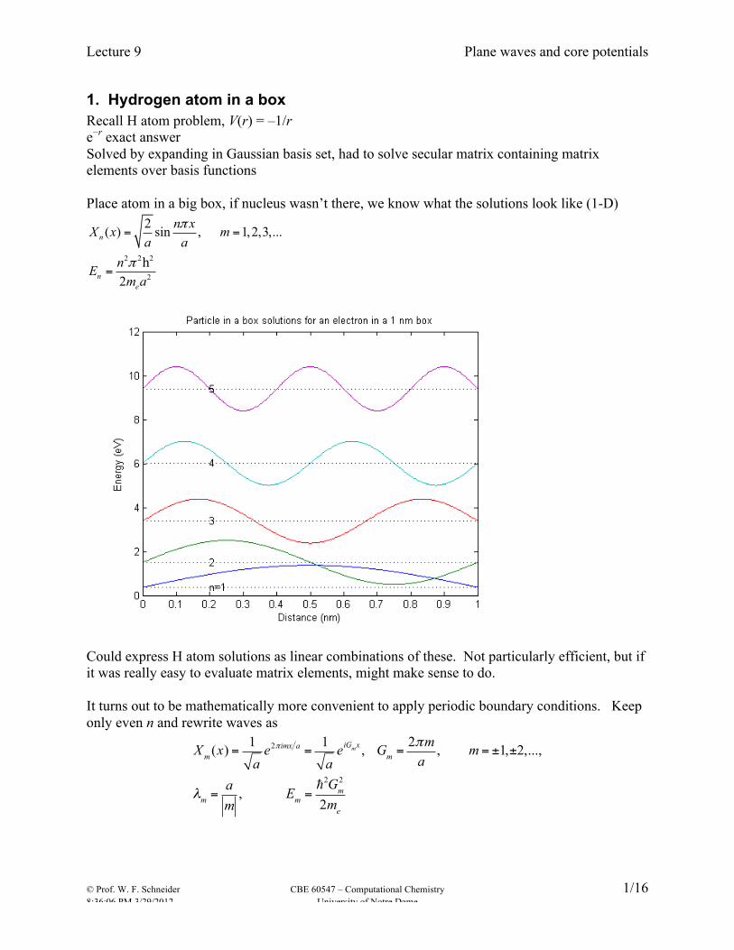
1. Hydrogen atom in a box Recall H atom problem, V(r) = –1/r e−r exact answer Solved by expanding in Gaussian basis set, had to solve secular matrix containing matrix elements over basis functions Place atom in a big box, if nucleus wasn’t there, we know what the solutions look like (1-D)
2
2
2 2
( ) sin , 1,2,32 ,...
2
n
ne
nX x ma
nE
xa
m a
π
π
= =
=h
Could express H atom solutions as linear combinations of these. Not particularly efficient, but if it was really easy to evaluate matrix elements, might make sense to do. It turns out to be mathematically more convenient to apply periodic boundary conditions. Keep only even n and rewrite waves as
Xm(x) =1ae2πimx a = 1
aeiGmx , Gm =
2πma, m = ±1,±2,...,
λm =am, Em =
2Gm2
2me
Lecture 9 Plane waves and core potentials
© Prof. W. F. Schneider CBE 60547 – Computational Chemistry 2/16 8:36:06 PM 3/29/2012 University of Notre Dame
(Ditto y and z.) Can write solutions for H atom as linear combination of these “plane wave” basis functions:
1 2( ,) miG xi im m
mG mx c e
aaπ
χ = =∑
If we let m run to infinity we would have a “complete” basis and could represent the H orbital exactly. In general we can’t keep an infinite number of m, so have to cut off somewhere, defined by
2Gm2
2me<2Gcut
2
2me= Ecutoff
Defines minimum wavelength retained in basis, and thus size m of basis. Note for a given Ecutoff, larger a implies bigger m. Within DFT, if we define a box size, an Ecutoff and a particular exchange-correlation functional, we’ve got ourselves a model!
−12d 2
dx2+υ(x)+υCoulomb(x)+υxc[ρ(x!)]
"
#$
%
&'ψi (x) = εiψi (x)
Kinetic energy: Diagonal in basis functions…easy!
( )2
22
1221
m miG x iG xm mm
ded
e Gx
δʹ′ʹ′− =
Potential energy terms: Can take advantage of Fourier transforms to evaluate:
1( ) ( ) ( ) ( )miG x iGxm m
mx G e G x e
adxυ υ υ υ −= =∑ ∫
( ) ( ) ( )m m m m miG x iG x iG x iG x iG xm m m
me x e G e e e Gυ υ υʹ′ ʹ′ʹ′ ʹ′
ʹ′ʹ′ ʹ′−ʹ′ʹ′
= =∑
How many Fourier components to include in the sums? Turns out for a basis of size m you need 2m components to specify the potential exactly, but you can get away with smaller. The cost and accuracy of the calculation scale with this choice.
2. Periodic boundary conditions Subtle but important point is that this approach is based on a periodic representation of a system; an artificial construction for something (like an atom or molecule) that isn’t actually periodic. Use the term supercell to describe periodic box. Have to make box large enough to avoid spurious interactions between periodic images.
Lecture 9 Plane waves and core potentials
© Prof. W. F. Schneider CBE 60547 – Computational Chemistry 3/16 8:36:06 PM 3/29/2012 University of Notre Dame
In particular, υ(x)+υCoulomb(x) is periodic and long-ranged, because it contains all the electrostatic 1/r terms. Have to use special tricks (Ewald summations) to evaluate these sums, and have to group electrostatic terms to avoid non-convergent sums. Key limitations of supercell approach (see Martin):
• Supercell must be net charge neutral (the electrostatic energy of an infinite, charged system diverges)
• Supercell must not have a net electric field • The absolute electrostatic potential is not well-defined (there is no “vacuum” to reference
an electron energy to in an infinite system). It is possible to overcome some of these limitations by introducing compensating background charges, dipoles, multipoles, …
3. Supercells – Cartesian and fractional coordinates Plane-wave calculations use periodic boundary conditions. Have to define two things to describe atomic arrangement: (1) Lattice constants of periodic cell, defined by three lattice vectors, a1, a2, a3
e.g., our cube for H, but could be any of the Bravais lattices, depending on the relationships between the three vectors
Every point R is equivalent to any other point R´= R + n1a1 + n2a2 + n3a3
(2) Locations of atoms within the periodic cell (the so-called “basis”)
Latter can be done by specifying locations of atoms in Cartesian coordinates r.
Typically easier to specify in fractional coordinates f of the lattice vectors.
Related by r = Af, where A is matrix generated by combining lattice vectors in column form.
4. Gaussian v. Vasp Compare Gaussian (6-311G(d,p)) and Vasp inputs and outputs for a spin-polarized PW91 H atom. Gaussian Vasp 1 input file 4 input files
POSCAR: structure input INCAR: program options POTCAR: identities of atoms KPOINTS: k-point sampling (more later)
z-matrix coordinates Atom positions relative to a supercell
Lecture 9 Plane waves and core potentials
© Prof. W. F. Schneider CBE 60547 – Computational Chemistry 4/16 8:36:06 PM 3/29/2012 University of Notre Dame
Arbitrary basis set Plane-wave cutoff Detailed options hidden Options “out there” Hartree units eV units 2 output files (.log and .chk) Lots of output files
OSZICAR: iteration summary OUTCAR: detailed output CONTCAR: final geometry
6 basis functions (6-311G(d,p)) 9045 basis functions (!!) (10 Å cube on a side, 250 eV cutoff)
3 cycles to converge (good initial guess)
15 cycles to converge (initial plane wave guess more difficult)
Spin-up and spin-down orbital eigenvalues
Spin-component “band” energies
Total energy referenced to ionized atom
Total energy referenced to…pseudopotential atomic state
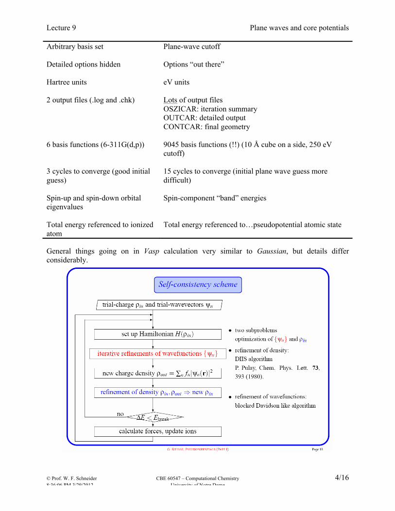
General things going on in Vasp calculation very similar to Gaussian, but details differ considerably.
Lecture 9 Plane waves and core potentials
© Prof. W. F. Schneider CBE 60547 – Computational Chemistry 5/16 8:36:06 PM 3/29/2012 University of Notre Dame
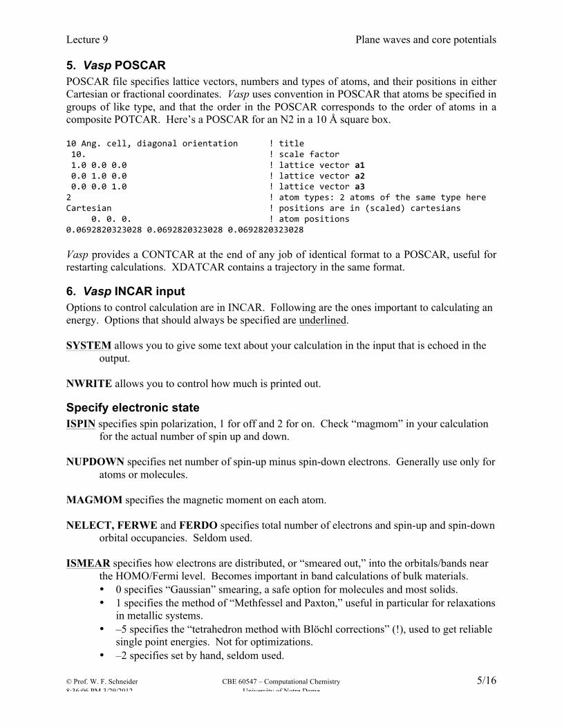
5. Vasp POSCAR POSCAR file specifies lattice vectors, numbers and types of atoms, and their positions in either Cartesian or fractional coordinates. Vasp uses convention in POSCAR that atoms be specified in groups of like type, and that the order in the POSCAR corresponds to the order of atoms in a composite POTCAR. Here’s a POSCAR for an N2 in a 10 Å square box. 10 Ang. cell, diagonal orientation ! title 10. ! scale factor 1.0 0.0 0.0 ! lattice vector a1 0.0 1.0 0.0 ! lattice vector a2 0.0 0.0 1.0 ! lattice vector a3 2 ! atom types: 2 atoms of the same type here Cartesian ! positions are in (scaled) cartesians 0. 0. 0. ! atom positions 0.0692820323028 0.0692820323028 0.0692820323028 Vasp provides a CONTCAR at the end of any job of identical format to a POSCAR, useful for restarting calculations. XDATCAR contains a trajectory in the same format.
6. Vasp INCAR input Options to control calculation are in INCAR. Following are the ones important to calculating an energy. Options that should always be specified are underlined. SYSTEM allows you to give some text about your calculation in the input that is echoed in the
output. NWRITE allows you to control how much is printed out.
Specify electronic state ISPIN specifies spin polarization, 1 for off and 2 for on. Check “magmom” in your calculation
for the actual number of spin up and down. NUPDOWN specifies net number of spin-up minus spin-down electrons. Generally use only for
atoms or molecules. MAGMOM specifies the magnetic moment on each atom. NELECT, FERWE and FERDO specifies total number of electrons and spin-up and spin-down
orbital occupancies. Seldom used. ISMEAR specifies how electrons are distributed, or “smeared out,” into the orbitals/bands near
the HOMO/Fermi level. Becomes important in band calculations of bulk materials. • 0 specifies “Gaussian” smearing, a safe option for molecules and most solids. • 1 specifies the method of “Methfessel and Paxton,” useful in particular for relaxations
in metallic systems. • –5 specifies the “tetrahedron method with Blöchl corrections” (!), used to get reliable
single point energies. Not for optimizations. • –2 specifies set by hand, seldom used.
Lecture 9 Plane waves and core potentials
© Prof. W. F. Schneider CBE 60547 – Computational Chemistry 6/16 8:36:06 PM 3/29/2012 University of Notre Dame
SIGMA sets the “smearing parameter,” which works hand-in-hand with ISMEAR. For
molecules and insulators, 0.05 eV is a sensible value; for metals 0.2 eV. Large values can help convergence but to large gives unphysical results. Aim to keep the electronic “entropy” (difference between free energy and total energy) < 1 meV/atom.
Precision parameters ENCUT specifies the plane wave energy cutoff, in eV. Vasp will select a default based on
ENMAX in the POTCAR, but much wiser to specify yourself. Max(ENMAX) over all the POTCARs is a safe default. Should in general test for convergence of properties of interest with ENCUT.
PREC specifies general precision of the calculation, including things like cut-off (ENCUT), the
accuracy of real-space core potential projections (LREAL), and the sizes of the FFT grids (NGX, NGY, NGZ). Use normal for normal stuff, accurate if you need high precision results.
LREAL specifies how to transform core potentials between reciprocal and real space. .FALSE.
(the default) says to do it exactly, good for small cells, but more expensive. “auto” says to create optimized real-space operators. Generally more efficient.
IDIPOL turns on “dipole corrections” to the total energy. Important only in calculations in
which the supercell has a large dipole moment. LORBIT is not a precision parameter, but it turns on printing out of charge analyses. –11 is a
good default value.
Self-consistent field parameters ALGO specifies the SCF algorithm. Note Vasp separates the problem into optimizations of the
wavefunction and the charge density. At the end of the SCF the two are consistent, but during the course of the SCF they are not. The default ALGO=fast uses a sequence of block diagonalization and DIIS methods that are, well, fast. ALGO=normal uses the safer but slower diagonalization method alone. In general SCF is more touchy for periodic systems. Never bother to calculate all orbitals (termed “bands”), only occupied and a few unoccupied.
NBANDS specifies how many bands (orbitals) to calculate. You always want to calculate all the
occupied ones and, for numerical reasons, at least some of the unoccupied ones. In general for performance reasons you don’t need or want to calculate all of the empty ones. The default is safe.
EDIFF specifies the SCF convergence criterion. 1e-4 for routine, 1e-5 for more accurate. NELM specifies maximum number of SCF cycles. If your calculation does not converge after the default number of steps, DO NOT just increase NELM!!!! Look carefully at change in energy, at the orbital occupancies, all the other computational details. Lack of convergence is telling you something!
Lecture 9 Plane waves and core potentials
© Prof. W. F. Schneider CBE 60547 – Computational Chemistry 7/16 8:36:06 PM 3/29/2012 University of Notre Dame
ISTART, INIWAV, ICHARG specify how to initialize the wavefunction and charge density.
Exchange-correlation parameters GGA specifies the DFT functional. The POTCARs are constructed for specific GGAs, and by default the exchange-correlation functional is determined from the POTCARs. LASPH determines how the exchange-correlation functional is evaluated in the core regions of atoms. Default is .FALSE., to evaluate using a spherical approximation. .TRUE. includes non-spherical contributions and should be used for magnetic centers, e.g. in oxides (Mike!). LHFCALC provides access to Hartree-Fock and “hybrid” functionals. This is very new and very expensive, so use only after careful study of the literature!
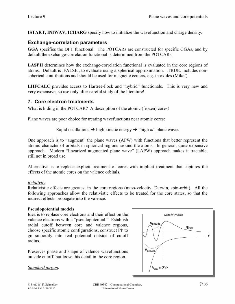
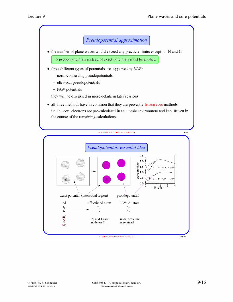
7. Core electron treatments What is hiding in the POTCAR? A description of the atomic (frozen) cores! Plane waves are poor choice for treating wavefunctions near atomic cores:
Rapid oscillations à high kinetic energy à “high m” plane waves One approach is to “augment” the plane waves (APW) with functions that better represent the atomic character of orbitals in spherical regions around the atoms. In general, quite expensive approach. Modern “linearized augmented plane wave” (LAPW) approach makes it tractable, still not in broad use. Alternative is to replace explicit treatment of cores with implicit treatment that captures the effects of the atomic cores on the valence orbitals. Relativity Relativistic effects are greatest in the core regions (mass-velocity, Darwin, spin-orbit). All the following approaches allow the relativistic effects to be treated for the core states, so that the indirect effects propagate into the valence. Pseudopotential models Idea is to replace core electrons and their effect on the valence electrons with a “pseudopotential.” Establish radial cutoff between core and valence regions, choose specific atomic configurations, construct PP to go smoothly into real potential outside of cutoff radius. Preserves phase and shape of valence wavefunctions outside cutoff, but loose this detail in the core region. Standard jargon: Vion ∝ Z/r
Vpseudo
ψreal
ψpseudo
Cutoff radius
r
Lecture 9 Plane waves and core potentials
© Prof. W. F. Schneider CBE 60547 – Computational Chemistry 8/16 8:36:06 PM 3/29/2012 University of Notre Dame
Transferability – ability of PP to be applied in different chemical environments Local vs. non-local – Spherically symmetric (local) vs. l-dependent (non-local) Norm-conserving – Preserving |ψ|2 of valence wavefunctions; important for getting long-range Coulomb potential correct Soft vs. hard –
Hard: closer to true atomic potential, requiring large KE cutoff Soft: larger perturbation on atomic potential, allowing smaller KE cutoff
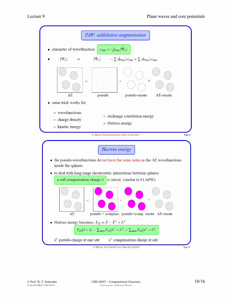
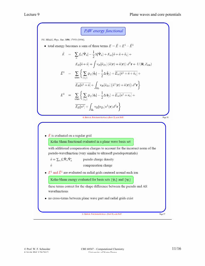
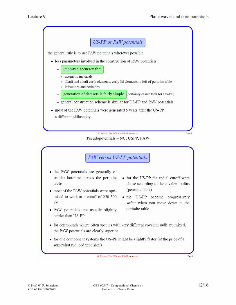
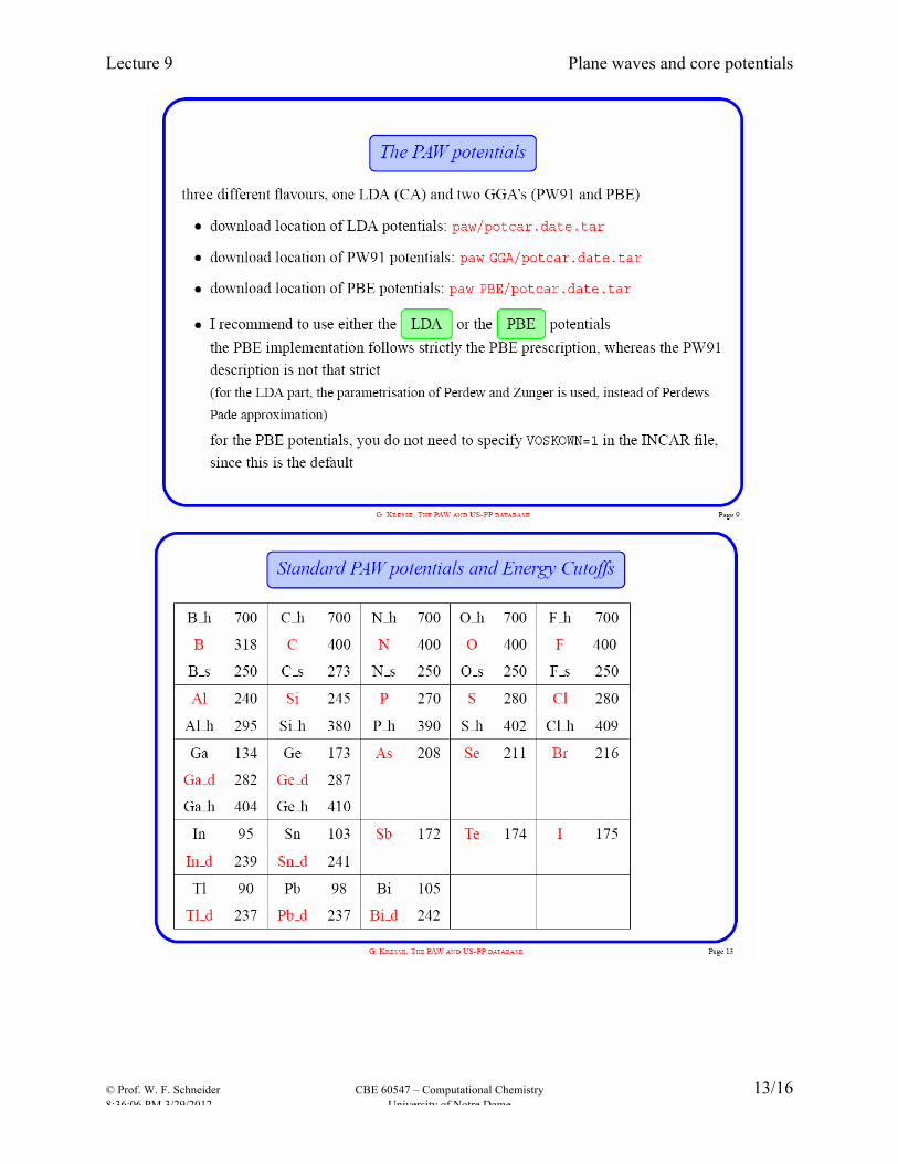
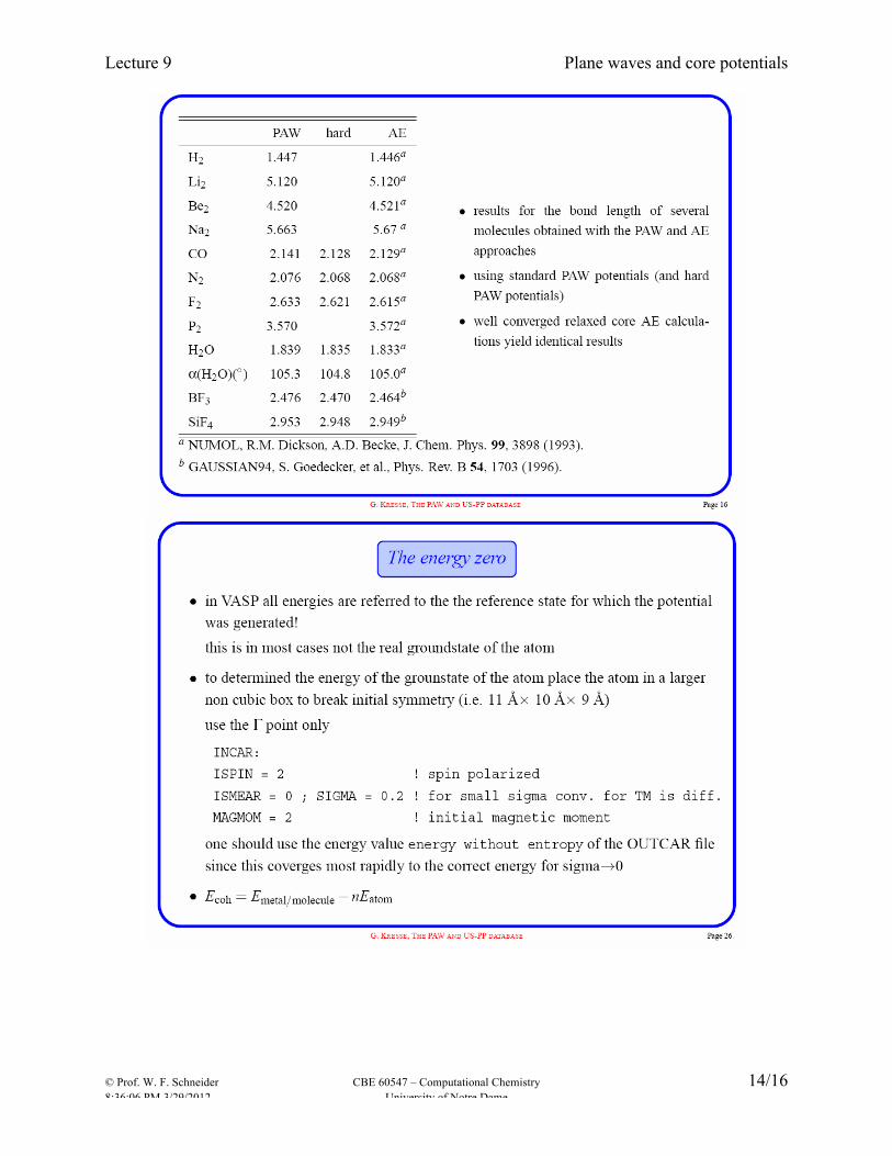
Ultra-soft (Vanderbilt) pseudo-potential: relax norm-conservation constraint to reduce cutoff, and compensate by putting “augmentation” charges on all atoms. These were the first potentials to enable efficient large-scale calculations. Projector augmented wave (PAW) PAW most modern approach, combines advantages of APW and of ultrasoft PPs. Not strictly a PP approach: constructs full wavefunction as combination of valence (plane wave) part and precomputed core parts from atomic calculations using same XC potential. Retains full nodal structure of valence wavefunctions. Generation of these potentials is not for the casual user (just as the case for making AO basis sets). The great strength of Vasp is a very complete and reliable library of potentials for the whole periodic table and for several exchange-correlation functional. Following slides borrowed from Georg Kresse presentation:
Lecture 9 Plane waves and core potentials
© Prof. W. F. Schneider CBE 60547 – Computational Chemistry 9/16 8:36:06 PM 3/29/2012 University of Notre Dame
Lecture 9 Plane waves and core potentials
© Prof. W. F. Schneider CBE 60547 – Computational Chemistry 10/16 8:36:06 PM 3/29/2012 University of Notre Dame
Lecture 9 Plane waves and core potentials
© Prof. W. F. Schneider CBE 60547 – Computational Chemistry 11/16 8:36:06 PM 3/29/2012 University of Notre Dame
Lecture 9 Plane waves and core potentials
© Prof. W. F. Schneider CBE 60547 – Computational Chemistry 12/16 8:36:06 PM 3/29/2012 University of Notre Dame
Pseudopotentials – NC, USPP, PAW
Lecture 9 Plane waves and core potentials
© Prof. W. F. Schneider CBE 60547 – Computational Chemistry 13/16 8:36:06 PM 3/29/2012 University of Notre Dame
Lecture 9 Plane waves and core potentials
© Prof. W. F. Schneider CBE 60547 – Computational Chemistry 14/16 8:36:06 PM 3/29/2012 University of Notre Dame
Lecture 9 Plane waves and core potentials
© Prof. W. F. Schneider CBE 60547 – Computational Chemistry 15/16 8:36:06 PM 3/29/2012 University of Notre Dame
8. Comparing energies between calculations When comparing energies between different calculations, e.g. to calculate reaction energies, must make sure to use the same cutoff, potentials, and all other key parameters underlined in section 5 in all calculations! Look for the “total energy” in the output.
9. Wavefunctions and charge densities As with any electronic structure calculation, the primary outputs are the total energy, the charge density, and the orbitals (or “bands”). Vasp provides some tools to look at these: Setting LCHARG=.TRUE. turns on creation of the CHGCAR, which contains the total charge density (and, for spin-polarized calculations, the spin-up minus spin-down density) evaluated on the NGX × NGY × NGZ grid. Not so interesting by itself, but by calculating a system and its parts identically in the same supercell, charge-density-differences can be created that show how charge “moves” when bonds are made. Setting LWAVE=.TRUE. turns on output of a WAVECAR, which includes everything about the final wavefunctions. Used primarily to restart calculations. LORBIT controls output of the DOSCAR and PROCAR which contain analysis of the total density of states and of each band, respectively. Controlled with RWIGS, EMIN, and EMAX. A supplementary code exists to extract Bader charges from the CHGCAR.
10. Exploring potential energy space Forces calculated using Hellman-Feynman theorem. No concern about Pulay forces (derivatives of basis functions wrt atom positions). Generally limited to Cartesian coordinates in supercell calculations—no internal coordinates, redundant coordinates. As with everything else, these can be more ill-behaved than Gaussian optimizations. There is an option in the POSCAR file to allow motions of only some of the atoms, called Selective Dynamics. Primarily useful when modeling surfaces.
Geometry optimizations IBRION = 2 turns on a conjugate-gradient optimization, safe but slower. IBRION = 1 turns on a quasi-Newton-Raphson, DIIS optimization. Uses a diagonal Hessian guess that
gets updates. Great close to minima or TS, hazardous otherwise. NFREE specifies how many previous steps to keep in the DIIS algorithm. Should always be less than the total number of degrees of freedom, and probably no bigger than 10.
IBRION = 3 turns on damped molecular dynamics, evidently good when you really have a bad intial
guess. I’ve neber tried it. NSW sets the maximum number of geometry steps. 0 means a single-point calculation, > 0 means an
optimization. EDIFFG determines the convergence criterion. > 0 means the optimization stops when the difference in
energy between two steps is < EDIFFG. < 0 means the optimization stops when the maximum force is < |EDIFFG| eV/Å. I prefer the latter. –0.05 is good for normal stuff, –0.03 for
Lecture 9 Plane waves and core potentials
© Prof. W. F. Schneider CBE 60547 – Computational Chemistry 16/16 8:36:06 PM 3/29/2012 University of Notre Dame
publication quality, might need even smaller if you want to calculate accurate frequencies. Note that the smaller EDIFFG is, the smaller EDIFF should be.
POTIM scales the forces that are used in the optimization. The efficiency of optimizations can be
sensitive to this. Start with the default 0.5, and if you are going to be doing a lot of calculations look at the manual for how to set more reliably.
ISW specifies whether to vary the atoms, the lattice vectors, or both. ISW = 1 just moves the atoms,
which is usually what you want.
Frequency calculations IBRION = 5 turns on a “dumb” numerical Hessian and frequency calculation that moves every atom
NFREE steps in the x, y, and z directions. NFREE = 2 gives 2-sided differences. POTIM specifies the step size, probably 0.01 or 0.015 Å.
IBRION = 6 turns on a smarter algorithm that takes advantage of any symmetry to cut down on the
number of force evaluations needed. IBRION = 7 and 8 turns on an analytical, perturbation-theory-based evaluation of the Hessian matrix.
Never tried it.
Molecular dynamics IBRION = 0 turns on molecular dynamics, when you just want to shake things up! MD is expensive, so
you will want to scale back on all your precision parameters, like PREC = low and a lower ENCUT. Better turn symmetry off (ISYM = 0).
NSW sets the number of MD steps, and POTIM the timestep in fs. SMASS = –3 turns on a simple NVE MD run; energy is conserved (or ought to be). SMASS = –1 turns on a scaled velocity MD. This allows you to do a simulated annealing, starting from a
high temperature and gradually cooling, or to roughly simulate a fixed temperature. NBLOCK controls the frequency with which the velocities are rescaled.
SMASS > 0 turns on an NVT MD run, and the value of SMASS specifies the thermostat mass. Ask an
expert. TEBEG, TEEND specify the initial and final temperatures in the MD run. Initial velocities are set
randomly according to TEBEG.


![BAS-300G INSTRUCTION MANUAL BAS-311G BAS … BAS-311G, BAS-326G iSAFETY INSTRUCTIONS [1] Safety indications and their meanings This instruction manual and the indications and symbols](https://img.pdfslide.us/doc/110x75/5ad1f1607f8b9a05208c18a3/bas-300g-instruction-manual-bas-311g-bas-bas-311g-bas-326g-isafety-instructions.jpg)