1

How you get from real data (points),

To continuous plots;

To power spectra analysis of the data.

2

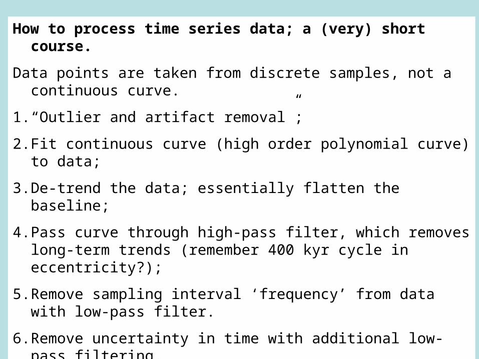
How to process time series data; a (very) short course.

Data points are taken from discrete samples, not a continuous curve.

1. “Outlier and artifact removal”;

2. Fit continuous curve (high order polynomial curve) to data;

3. De-trend the data; essentially flatten the baseline;

4. Pass curve through high-pass filter, which removes long-term trends (remember 400 kyr cycle in eccentricity?);

5. Remove sampling interval ‘frequency’ from data with low-pass filter.

6. Remove uncertainty in time with additional low-pass filtering.

7. “Reflect” data at both ends of the curve – to avoid high frequency ‘ringing’.

Now – do spectral analysis on resulting curve.

3

CO2 flux to/from the oceans is NOT uniform.

Some areas have input, some have output.

4

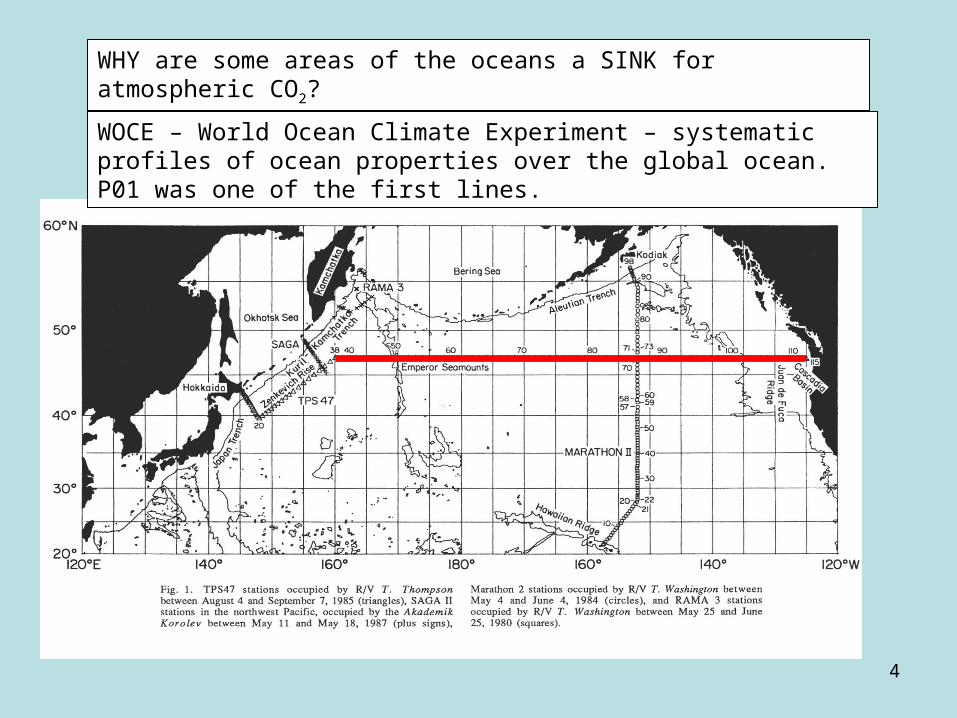
WOCE – World Ocean Climate Experiment – systematic profiles of ocean properties over the global ocean. P01 was one of the first lines.

WHY are some areas of the oceans a SINK for atmospheric CO2?

5

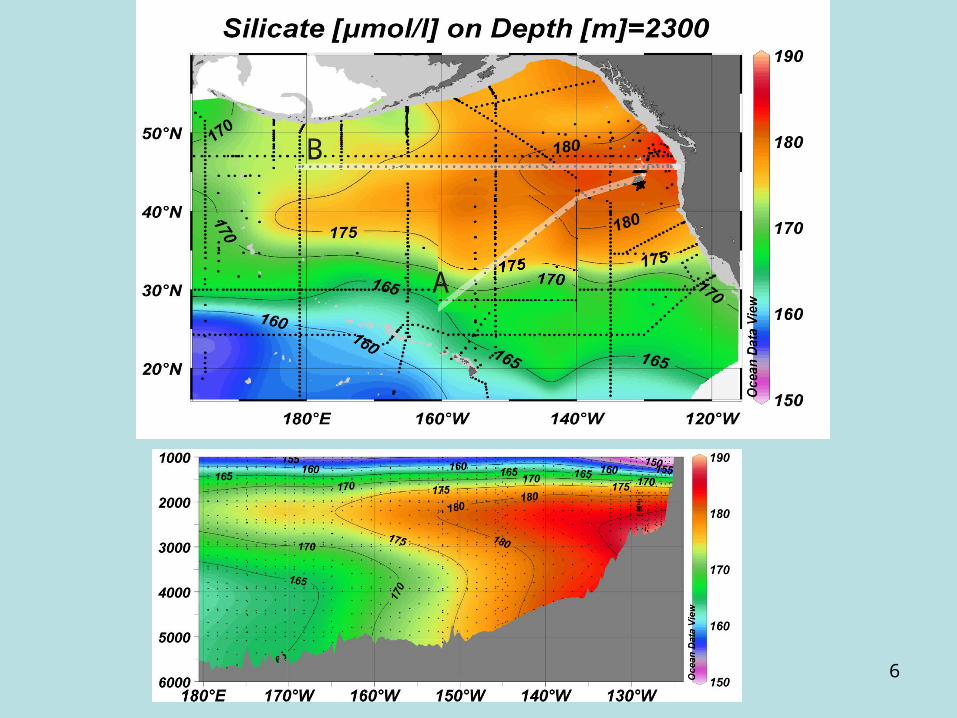
Talley and Joyce, JGR, 1992 – Dissolved Si plume across the N. Pacific

N.AmericaSiberia

N. Pacific sea floor

6

A

B

7

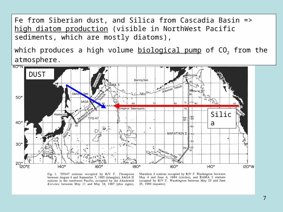
Fe from Siberian dust, and Silica from Cascadia Basin => high diatom production (visible in NorthWest Pacific sediments, which are mostly diatoms),

which produces a high volume biological pump of CO2 from the atmosphere.

DUST

Silica

8

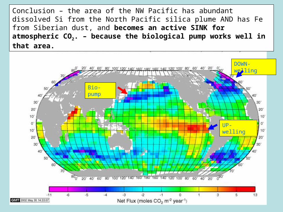
Conclusion – the area of the NW Pacific has abundant dissolved Si from the North Pacific silica plume AND has Fe from Siberian dust, and becomes an active SINK for atmospheric CO2. – because the biological pump works well in that area.

DOWN- welling

Bio-pump

UP- welling

9

Antarctic Record of CO2 and Temperature

Eemian interglacial

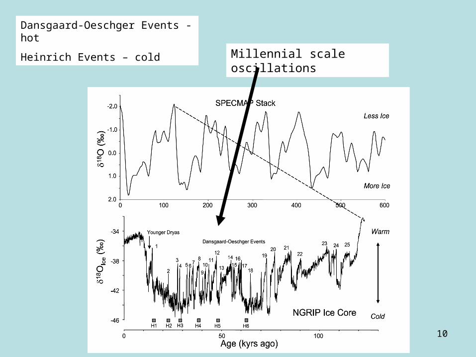
Millennial scale oscillationsYounger Dryas

10

Millennial scale oscillations

Dansgaard-Oeschger Events - hot

Heinrich Events – cold

11

Eemian Interglacial period

12

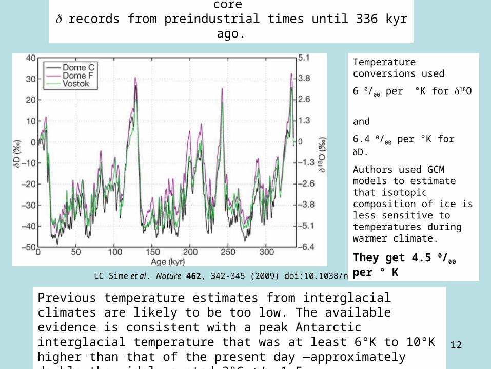
LC Sime et al. Nature 462, 342-345 (2009) doi:10.1038/nature08564

Time series of Dome C, Dome F and Vostok ice core records from preindustrial times until 336 kyr ago.

Previous temperature estimates from interglacial climates are likely to be too low. The available evidence is consistent with a peak Antarctic interglacial temperature that was at least 6°K to 10°K higher than that of the present day —approximately double the widely quoted 3°C +/- 1.5

Temperature conversions used

6 0/00 per °K for 18O

and

6.4 0/00 per °K for D.

Authors used GCM models to estimate that isotopic composition of ice is less sensitive to temperatures during warmer climate.

They get 4.5 0/00 per ° K

13

How does the Eemian atmosphere compare to the PRESENT one?

14

Records of sea level change during the Eemian Last Interglacial period are about 5 meters HIGHER THAN PRESENT– associated with a 3.50 temperature increase.

There is considerable debate in the paleo-climate community about WHERE THIS WATER IS COMING FROM.

Recent studies indicate that much (most) of this came from the melting of the Greenland ice sheet.

15

Last Glacial Maximum (~20K yrs ago) and afterwards

• What was climate like during LGM?• What happened to end LGM?• How has climate varied since LGM?• What were the likely mechanisms of climate

change?

16

Ice Sheet Extent

• Laurentide, Cordilleran and Scandinavian Ice Sheets

• Areal extent at LGM reconstructed by 14C dated end moraines (25% of land covered at LGM vs 10% today).

• Thickness of ice sheets is harder to estimate than area.

17

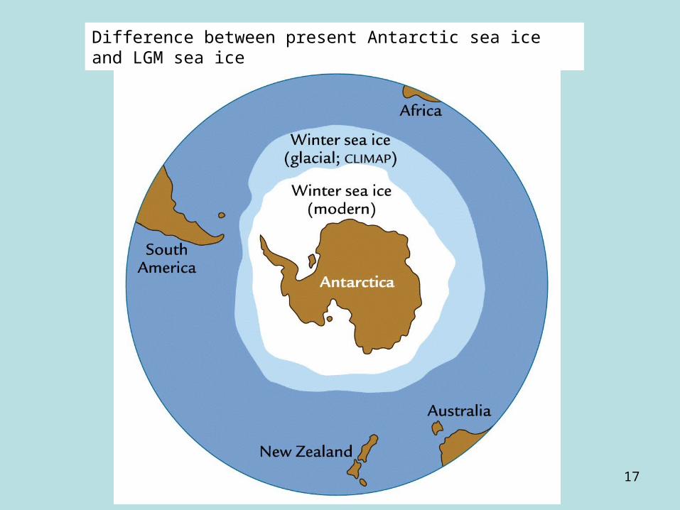
Difference between present Antarctic sea ice and LGM sea ice

18

How thick were

the ice sheets?

Two models – thick (early) and thin (more recent). Thickness determination is difficult: 30% of ice is buried below level plane. Thicknesses are now contrained by sealevel estimates and new ice flow (cemented vs free base) models.

19This ‘rebound’ from past glacial loading can confuse measurements of present sea level change.

20

How do we determine the volume of the LGM Ice Sheet?

1. From sea level rise;

2. Glacial moraines give lateral extent (but not thickness)

3. ‘Rebound’ of the depressed continent beneath the ice sheet (cm/year) can be used to estimate thickness.

continent

ice 70%

30%

21

Post-glacial rebound. If bottom of ice sheet is depressed (buried) below the initial level surface, and then the ice sheet melts, the land mass will rebound to the original height. 14C dating of the old beach marks (as the land rose) allow estimates of this rebound rate. 150 m/7000 yrs = 2 cm/year.

Hudson Bay paleo-beach

22

LC Sime et al. Nature 462, 342-345 (2009) doi:10.1038/nature08564

Time series of Dome C, Dome F and Vostok ice core records from preindustrial times until 336 kyr ago.

Previous temperature estimates from interglacial climates are likely to be too low. The available evidence is consistent with a peak Antarctic interglacial temperature that was at least 6°K to 10°K higher than that of the present day —approximately double the widely quoted 3°C +/- 1.5

Temperature conversions used

6 0/00 per °K for 18O

and

6.4 0/00 per °K for D.

Authors used GCM models to estimate that isotopic composition of ice is less sensitive to temperatures during warmer climate.

They get 4.5 0/00 per ° K

23

Eemain Interglacial period

perhaps the BEST analog of future climate change.

•Temperature peak for the Eemian occurred about 125,000 years BP,

•Global temperatures were about 3.5 deg C warmer than present (new Sime et al data says 3 to 5°C warmer).

•In Europe, where data is really good, pollen from drill cores indicates that temperature forests moved into areas that are now arctic tundra.

•Which translates to about 7 to 8 deg C higher in the Arctic latitudes.

•Note that current model estimates are that arctic temperatures only have to be 5 to 8 deg C higher – to melt the Greenland ice cap…

•Eemian sea level estimated to be 6 to 7 m higher than present…

24

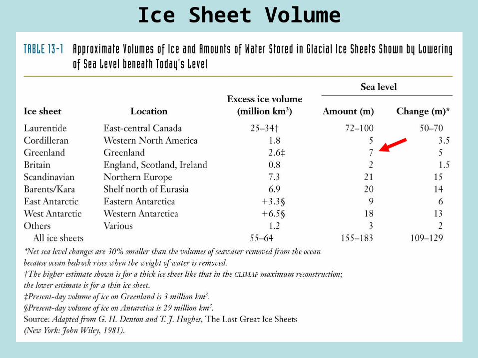
Ice Sheet Volume

25

How do we determine the volume of the LGM Ice Sheet?

1. From sea level rise;

2. Glacial moraines give lateral extent (but not thickness)

3. ‘Rebound’ of the depressed continent beneath the ice sheet (cm/year) can be used to estimate thickness.

continent

ice 70%

30%

26

During the Eemian Interglacial period, global sea level was ~6 to 7 meters higher than present. Where did this water come from?

Previous models indicated that it came from West Antarctic Ice Sheet, but

New Models indicate that most (~4 to 5.5 m) came from Greenland Ice Sheet.

Where the water came from (for the 7 m SL rise) depends on the value of , the constant of proportionality between 18O and temperature,

For Greenland.

Recent modeling results suggest a different value of a than previously used.

Previous values = 0.67 0/00 per °C.

NEW values = 0.4 0/00 per °C.

Assume 10 0/00 change at Eemian interglacial.

27

Assume 10 0/00 change at Eemian interglacial

Previous values = 0.67 0/00 per °C.

T for 10 0/00 = (10)/(0.67) = 15°C change.

NEW values = 0.4 0/00 per °C. for Greenland!

T for 10 0/00 = (10)/(.4) = 25°C

or 10°C warmer than previous models!.

old

new

28

Surface elevation maps for the Greenland ice sheet at its Eemian minimum.

Maps of three different values for a. Map b is preferred. Map c is consistent with previous modeling efforts.

Center of Ice Dome was only 200 to 300 m lower during Eemian than present summit.

New model that produced higher temperatures was based on local atmospheric environment, and not global values.

Greenland ice sheet would have melted ‘around the edges’, while maintaining central core of ice.(Cuffey and Marshall, Nature, 404, 2000).

29

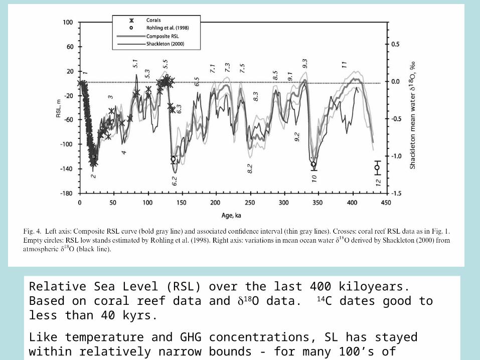
Relative Sea Level (RSL) over the last 400 kiloyears. Based on coral reef data and 18O data. 14C dates good to less than 40 kyrs.

Like temperature and GHG concentrations, SL has stayed within relatively narrow bounds - for many 100’s of thousands of years.

30

Wave-cut terraces on San Clemente Island, California.

Nearly horizontal surfaces, separated by step-like cliffs, were created during former intervals of high sea level; the highest terrace represents the oldest sea-level high stand.

Because San Clemente Island is slowly rising, terraces cut during an interglacial continue to rise with the island during the following glacial interval.

31

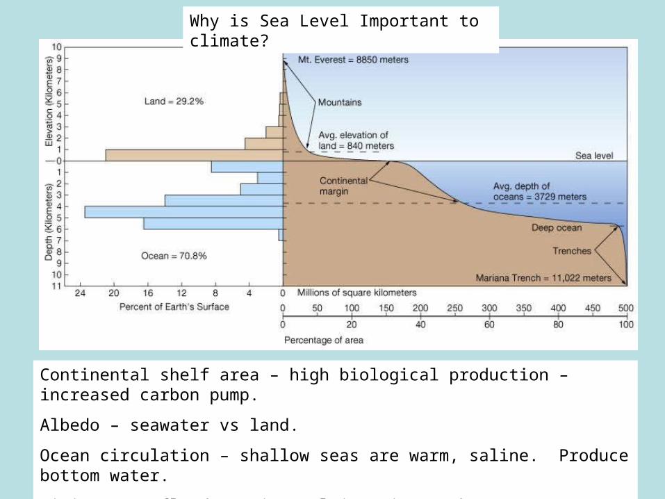
Why is Sea Level Important to climate?

Continental shelf area – high biological production – increased carbon pump.

Albedo – seawater vs land.

Ocean circulation – shallow seas are warm, saline. Produce bottom water.

Rising seas flood continental interiors; change precipitation patterns.

32

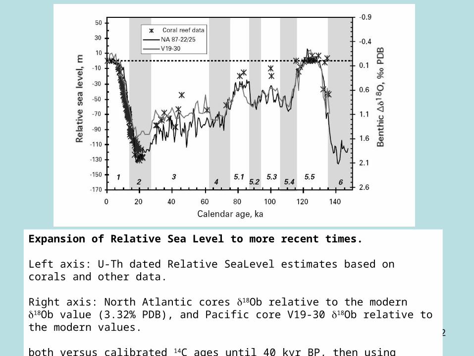
Expansion of Relative Sea Level to more recent times.

Left axis: U-Th dated Relative SeaLevel estimates based on corals and other data.

Right axis: North Atlantic cores 18Ob relative to the modern 18Ob value (3.32% PDB), and Pacific core V19-30 18Ob relative to the modern values.

both versus calibrated 14C ages until 40 kyr BP, then using SPECMAP isotope data for older ages.

33

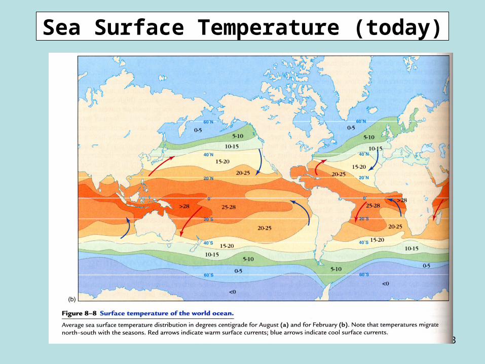
Sea Surface Temperature (today)

34

Sea Surface Temperature Change at LGM

35

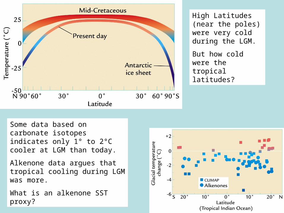
High Latitudes (near the poles) were very cold during the LGM.

But how cold were the tropical latitudes?

Some data based on carbonate isotopes indicates only 1° to 2°C cooler at LGM than today.

Alkenone data argues that tropical cooling during LGM was more.

What is an alkenone SST proxy?

36

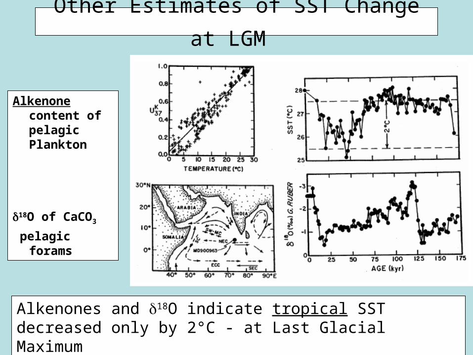
Other Estimates of SST Change at LGM

Alkenone content of pelagic Plankton

18O of CaCO3

pelagic forams

Alkenones and 18O indicate tropical SST decreased only by 2°C - at Last Glacial Maximum

37

38

e. Huxleyieveryones favorite

What is an alkenone?

A saturated fat used by phytoplankton (for cell walls, interior fluid).

The degree of saturation (number of carbon-hydrogen bonds) in these fats depends on temperature. HIGH saturation fats become solid at low temperatures (like lard).

So extraction of these alkenones from plankton in sediments (specific species), and measurement of their degree of ‘saturation’, can give the temperature at which the formed.

ALKENONES; a proxy for seawater temperatures –

without needing to know ice volume!

39

What is a saturated fat?

Changing the degree of saturation changes the physical properties of the fat, including their viscosity (ability to flow) and melting temperature

40

Saturated fat Unsaturated fattransfat –

Not climate related

Olive oil

41

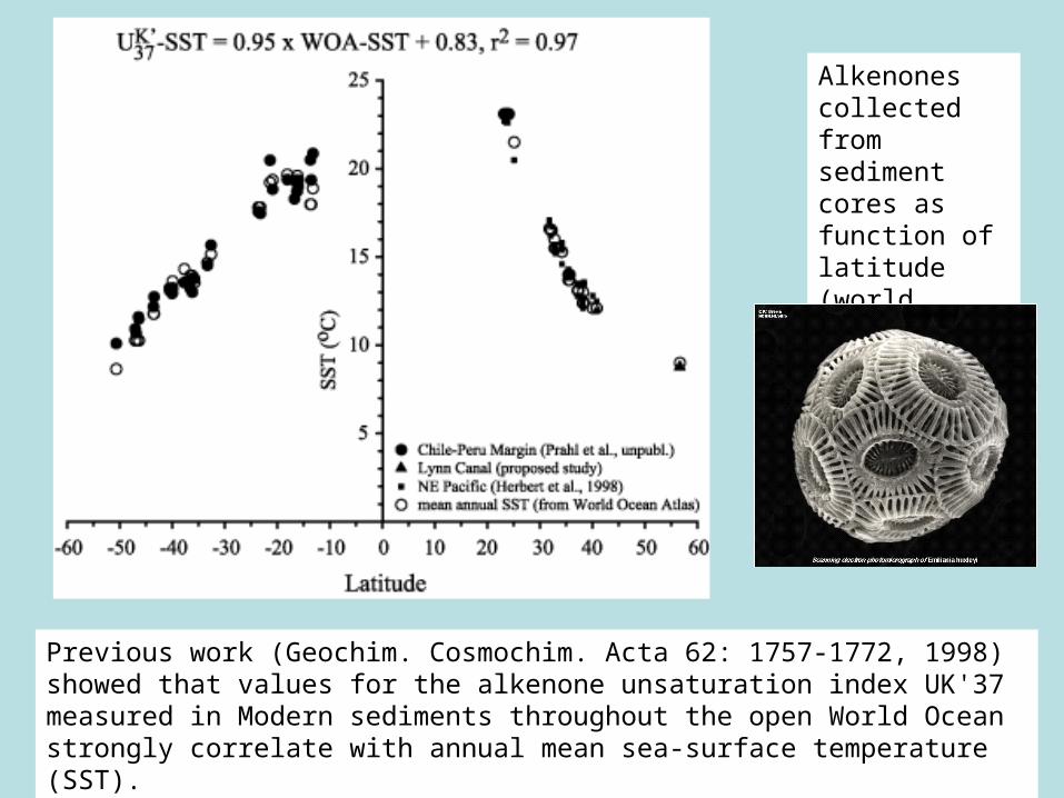
Previous work (Geochim. Cosmochim. Acta 62: 1757-1772, 1998) showed that values for the alkenone unsaturation index UK'37 measured in Modern sediments throughout the open World Ocean strongly correlate with annual mean sea-surface temperature (SST).

Alkenones collected from sediment cores as function of latitude (world wide).

42

So by

•Picking out individual species of phytoplankton from sediment cores.

•extraction of alkenones (using organic solvents) from these skeletons

•Running the extractions in a gas chromatograph – to get the specific fat saturated to unsaturated ratio

•It is possible to get sea water temperatures (benthic or pelagic) when the phytoplankton grew

WITHOUT THE NEED TO KNOW ICE VOLUME.

43

ALKENONE record of SST off Santa Barbara, CA

Comparing 18O with alkenone seawater temperatures

44

So if you do alkenone extraction and analysis from sediments (i.e., take a series of cores along a profile along a longitude)

that are LGM in age in the tropics, you can estimate the sea surface temperature – in the tropics – at LGM time.

And that is quite small (i.e., the equator didn’t get very cold at LGM although the poles and intermediate latitudes did).

45

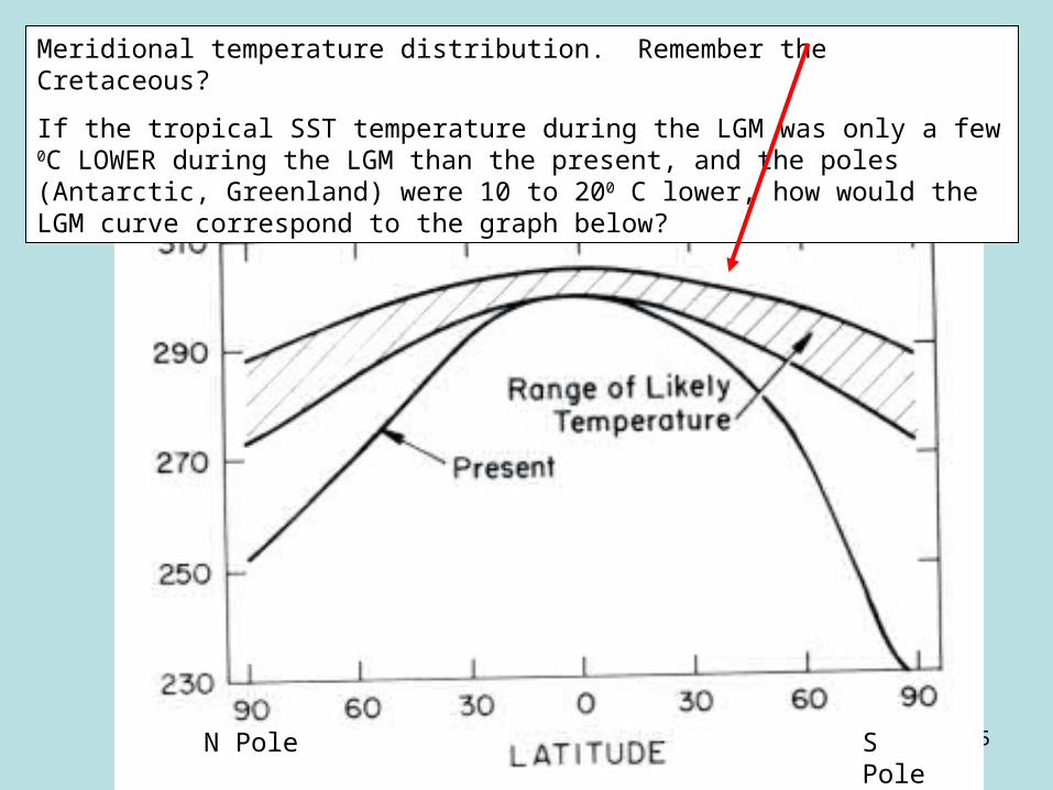
Meridional temperature distribution. Remember the Cretaceous?

If the tropical SST temperature during the LGM was only a few 0C LOWER during the LGM than the present, and the poles (Antarctic, Greenland) were 10 to 200 C lower, how would the LGM curve correspond to the graph below?

N Pole S Pole

46

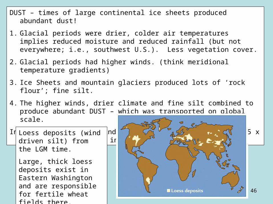
DUST – times of large continental ice sheets produced abundant dust!

1. Glacial periods were drier, colder air temperatures implies reduced moisture and reduced rainfall (but not everywhere; i.e., southwest U.S.). Less vegetation cover.

2. Glacial periods had higher winds. (think meridional temperature gradients)

3. Ice Sheets and mountain glaciers produced lots of ‘rock flour’; fine silt.

4. The higher winds, drier climate and fine silt combined to produce abundant DUST – which was transported on global scale.

Indian Ocean sediments indicate that LGM dust levels were 5 x higher than present – in that area.

Loess deposits (wind driven silt) from the LGM time.

Large, thick loess deposits exist in Eastern Washington and are responsible for fertile wheat fields there.

47

Desert dust source regions today –

Arrows are prevailing winds today: during LGM, these areas produced even MORE dust than they are today. Note: dust from the Sahara desert is blown out into the south Atlantic, providing IRON that fertilizes upper ocean productivity

48

Regions with abundant sand dunes during:

Top – today.

Bottom – LGM time.

Dust levels in Antarctica were 10 x those today, as estimated from the ice cores.

If surface ocean biology (diatoms vs coccolithophores) plays a role in the transition from glacial to interglacial periods…

By INCREASING the biological PUMP

it is likely to be through ocean circulation – and dust (as a nutrient supply).

49

Climate change near the North American Ice Sheets:

Near the edge of the ice sheets, the climate was much wetter than present; with Lake Bonneville (covered 40% of the State of Utah) being an example.

Lake Bonneville existed about 15K years ago, and drained catastrophically into the Columbia River when the natural dam in the north failed.

This drainage may (or may not) have produced changes in the ocean circulation in the NE Pacific Ocean – along with Lake Missoula floods.

In contrast to the SW, the Pacific NW was colder and drier, and many areas were desert.

50

Jet stream in modern times: note it is just north of Seattle.

Jet stream (from numerical models) during Last Glacial Maximum: note that it is considerably farther south.

51

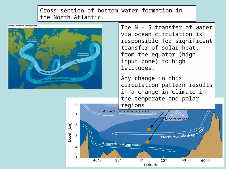
Cross-section of bottom water formation in the North Atlantic.

The N - S transfer of water via ocean circulation is responsible for significant transfer of solar heat, from the equator (high input zone) to high latitudes.

Any change in this circulation pattern results in a change in climate in the temperate and polar regions

52

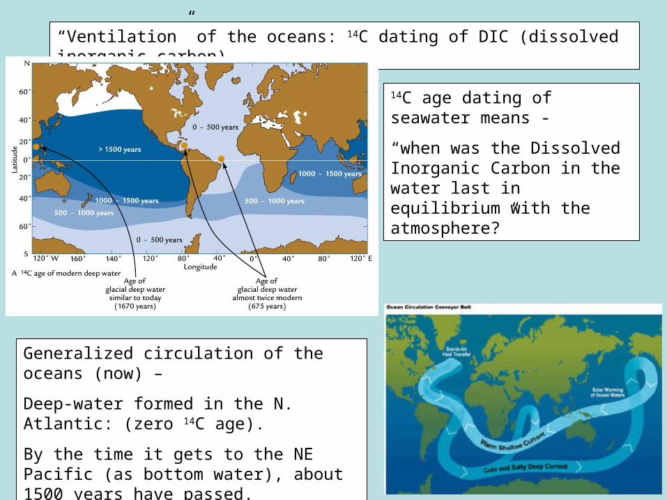
“Ventilation” of the oceans: 14C dating of DIC (dissolved inorganic carbon)

14C age dating of seawater means -

“when was the Dissolved Inorganic Carbon in the water last in equilibrium with the atmosphere?”

Generalized circulation of the oceans (now) –

Deep-water formed in the N. Atlantic: (zero 14C age).

By the time it gets to the NE Pacific (as bottom water), about 1500 years have passed.

53

14C dating of DIC (dissolved inorganic carbon)

Dissolved inorganic carbon in seawater.

HCO3– (1777 mol/kg) and CO3= (225 mol/kg). So mostly bicarbonate.

Some of these carbon atoms are the isotope 14C, which is formed in the atmosphere from cosmic ray bombardment, and decays which with a half life (50% gone) of 5,730 years.

Probably can measure out to 6 half-lives, or 30,000 years.

DIC can be obtained from water samples taken from the top and bottom of the water column.

By carefully measuring the “14C age” of this DIC and comparing surface and benthic values, it is possible to get an estimate of the number of years since that bottom water was exposed on the surface.

54

14C

Ocean convection cell: if convection is FAST, then surface and deep water will have (about) the same values of 14C.

If the convection cell is slow (stopped), surface and bottom water will have very different 14C values.

Young 14C

Old (decayed) 14C

55

By measuring the 14C values in sediments in benthic and pelagic forams – as a function of sediment age, it is possible to estimate the ‘vigor’ of ocean circulation at different times (i.e., during the present, and during the LGM).

In the Pacific, the age difference (benthic vs pelagic) is similar to today;

In the equatorial Atlantic, the age difference was about twice (675 years) the modern value of 350 years.

This means bottom water circulation in the Atlantic at LGM was slower than today – i.e, less bottom water formation at high latitudes.

This means that during the LGM, less thermal energy was transferred from the equatorial Atlantic to the north Atlantic; with strong implications for climate in the northern hemisphere.

The area around Paris, for instance, became arctic tundra.

56

Deep Water Formation: Present vs LGM

57

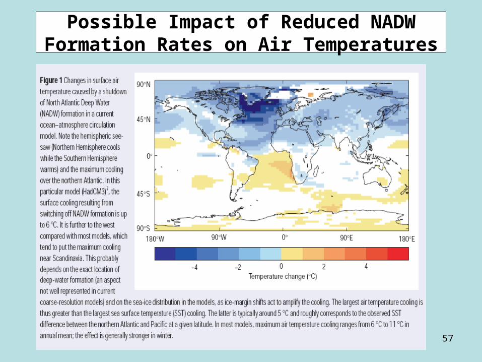
Possible Impact of Reduced NADW Formation Rates on Air Temperatures

58

Vegetation Changes

Use pollen records from several lakes to reconstruct regional vegetation distribution during LGM.

NOW

LGM

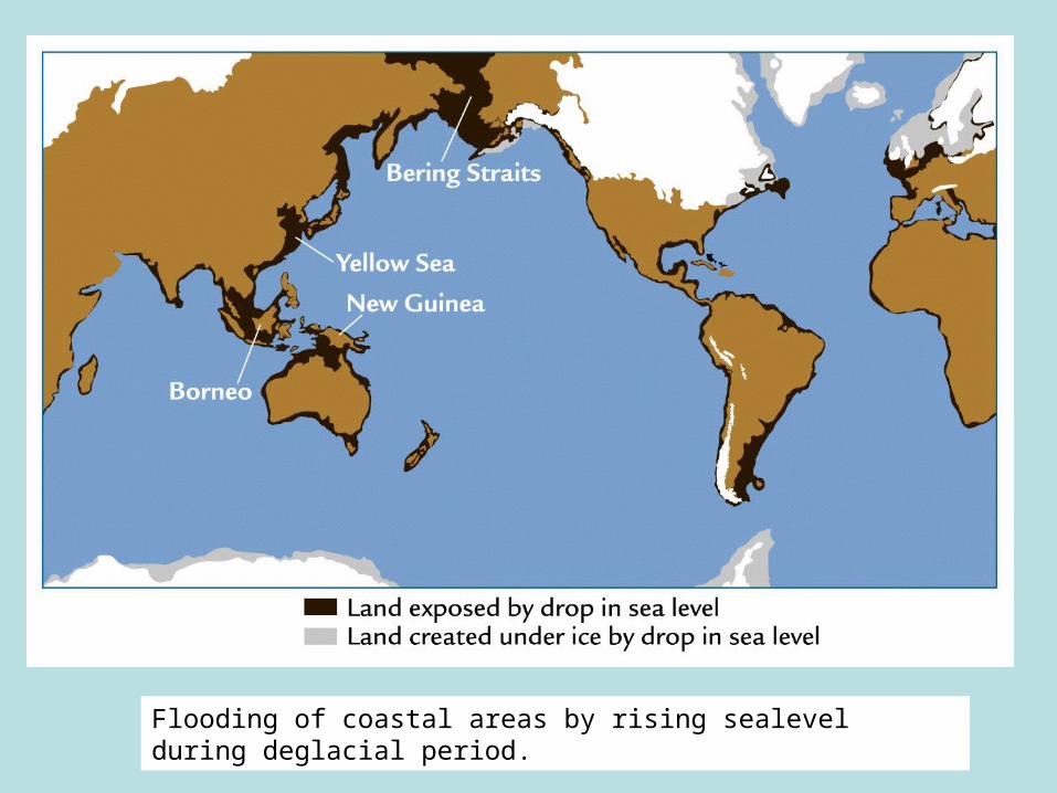
Flooding of coastal areas by rising sealevel during deglacial period.

60

Atmospheric Gases during LGM

CO2 was 180 ppm (vs 280 ppm at warm interglacials)

CH4 was ~350 ppb (vs 700 ppb at interglacials)

61

Summary: Climate Conditions during LGM

• Insolation rates about the same as today.• Colder (~ -4 º C globally and ~ -10 ºC near

the poles (maybe colder) and ~-2 to -3 ºC in tropics).• Ice Sheet volume was ~ twice today.• Sea Level lower by ~ 125m.• Drier and dustier (globally).

• Reduced atmospheric CO2 and CH4 levels

• Vegetation more arctic like (tundra, steppe).

• Deep Ocean circulation more sluggish.

62

Ice Sheet Retreat

Ice Sheet retreat begins about 18 -14 kyrs ago, and are largely gone by 6,000 years ago.

63

Sea Level Rise

• Use 14C and 230Th/238U to date the age of a sequence of submerged corals that lived close to the sea surface.

• The rate of sea level rise has pulses.

(14C ages are too young by up to ~3K yrs.)

What have we covered so far – the Basic Questions

1. Climate has not always been similar to the present; in fact has rarely been like the present Holocene climate.

2. Climate depends on a large number of variables - with abundant feedbacks, and climate change is not necessarily intuitive.

3. The scientific community does not understand some basics about climate, even for recent periods where the data are good. This includes the causes of the glacial/interglacial cycles.

4.Climate change can be both dramatic, and fast: the return to glacial climate during the Younger Dryas may have happened in just a few decades.

5. Computer models are just (digital) plausibility arguments, and are limited by our understanding of what are the important variables, in resolution, and in ability to predict the future.

Summary: Climate Conditions during Last Glacial Maximum

• Insolation rates about the same as today.

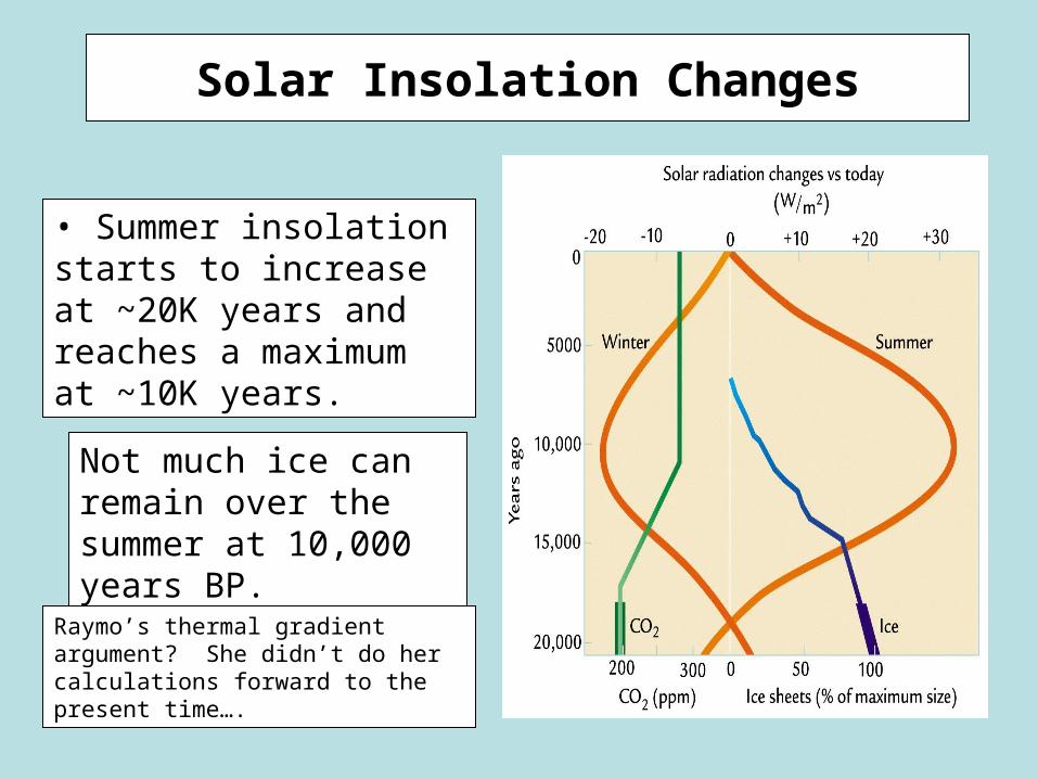
Solar Insolation Changes

• Summer insolation starts to increase at ~20K years and reaches a maximum at ~10K years.

Not much ice can remain over the summer at 10,000 years BP.

Raymo’s thermal gradient argument? She didn’t do her calculations forward to the present time….

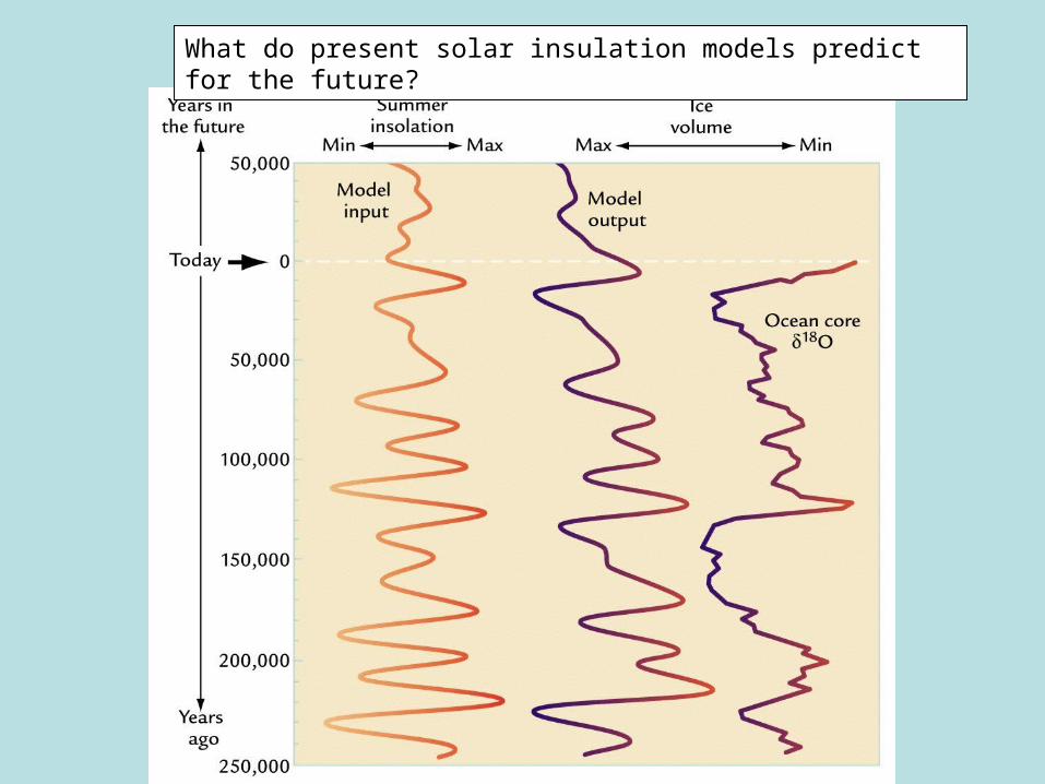
What do present solar insulation models predict for the future?

Summary: Climate Conditions during LGM

• Insolation rates about the same as today.• Colder (~ -4 º C globally and ~ -10 ºC (or –

20) near the poles and ~-2 to -3 ºC in tropics).• Ice Sheet volume was ~ twice today.• Sea Level lower by ~ 125m. Exposed large

continental shelf areas.• Drier and dustier (globally).• Reduced atmospheric CO2 and CH4 levels• Vegetation more arctic like (tundra, steppe).• Deep Ocean circulation more sluggish.

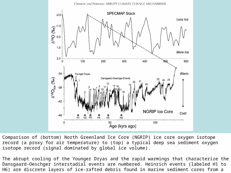
Comparison of (bottom) North Greenland Ice Core (NGRIP) ice core oxygen isotope record (a proxy for air temperature) to (top) a typical deep sea sediment oxygen isotope record (signal dominated by global ice volume).

The abrupt cooling of the Younger Dryas and the rapid warmings that characterize the Dansgaard-Oeschger interstadial events are numbered. Heinrich events (labeled H1 to H6) are discrete layers of ice-rafted debris found in marine sediment cores from a wide swath of the subpolar North Atlantic. They have been interpreted to reflect the episodic discharge of massive numbers of icebergs from the Hudson Strait region.