Embed Size (px)
Citation preview
1
Histograms and Wavelets
on Probabilistic DataGraham Cormode, AT&T Labs Research
Minos Garofalakis, Technical University of Crete
Email: [email protected], [email protected]
F
Abstract
There is a growing realization that uncertain information is a first-class citizen in modern database management.
As such, we need techniques to correctly and efficiently process uncertain data in database systems. In particular, data
reduction techniques that can produce concise, accurate synopses of large probabilistic relations are crucial. Similar to
their deterministic relation counterparts, such compact probabilistic data synopses can form the foundation for human
understanding and interactive data exploration, probabilistic query planning and optimization, and fast approximate query
processing in probabilistic database systems.
In this paper, we introduce definitions and algorithms for building histogram- and Haar wavelet-based synopses on
probabilistic data. The core problem is to choose a set of histogram bucket boundaries or wavelet coefficients to optimize
the accuracy of the approximate representation of a collection of probabilistic tuples under a given error metric. For a
variety of different error metrics, we devise efficient algorithms that construct optimal or near optimal size B histogram and
wavelet synopses. This requires careful analysis of the structure of the probability distributions, and novel extensions of
known dynamic-programming-based techniques for the deterministic domain. Our experiments show that this approach
clearly outperforms simple ideas, such as building summaries for samples drawn from the data distribution, while taking
equal or less time.
Index Terms
Histograms, wavelets, uncertain data
1 INTRODUCTION
Modern real-world applications generate massive amounts of data that is often uncertain and imprecise. For
instance, data integration and record linkage tools can produce distinct degrees of confidence for output
data tuples (based on the quality of the match for the underlying entities) [8]; similarly, pervasive multi-
sensor computing applications need to routinely handle noisy sensor/RFID readings [25]. Motivated by
these new application requirements, recent research on probabilistic data management aims to incorporate
uncertainty and probabilistic data as “first-class citizens” in the DBMS.
DRAFT
2
Among different approaches for modeling uncertain data, tuple- and attribute-level uncertainty models
have seen wide adoption both in research papers as well as early system prototypes [1], [2], [3]. In such
models, the attribute values for a data tuple are specified using a probability distribution over different
mutually-exclusive alternatives (that might also include non-existence, i.e., the tuple is not present in the
data), and assuming independence across tuples. The popularity of tuple-/attribute-level uncertainty
models is due to their ability to describe complex dependencies while remaining simple to represent
in current relational systems, with intuitive query semantics. In essence, a probabilistic database is a
concise representation for a probability distribution over an exponentially-large collection of possible
worlds, each representing a possible “grounded” (deterministic) instance of the database (e.g., by flipping
appropriately-biased independent coins to select an instantiation for each uncertain tuple). This “possible-
worlds” semantics also implies clean semantics for queries over a probabilistic database—essentially,
the result of a probabilistic query defines a distribution over possible query results across all possible
worlds [8]. The goal of query answering over uncertain data is to provide the expected value of the
answer, or tail bounds on the distribution of answers.
Unfortunately, despite its intuitive semantics, the paradigm shift towards tuple-level uncertainty also
implies computationally-intractable #P -hard data complexity even for simple query processing opera-
tions [8]. These negative complexity results for query evaluation raise serious practicality concerns for
the applicability of probabilistic database systems in realistic settings. One possible avenue of attack is
via approximate query processing techniques over probabilistic data. As in conventional database systems,
such techniques need to rely on appropriate data reduction methods that can effectively compress large
amounts of data down to concise data synopses while retaining the key statistical traits of the original
data collection [10]. It is then feasible to run more expensive algorithms over the much compressed
representation, and obtain a fast and accurate answer. In addition to enabling fast approximate query
answers, over probabilistic data, such compact synopses can also provide the foundation for human
understanding and interactive data exploration, and probabilistic query planning and optimization.
The data-reduction problem for deterministic databases is well understood, and several different syn-
opsis construction tools exist. Histograms [20] and wavelets [4] are two of the most popular general-purpose
data-reduction methods for conventional data distributions. It is hence meaningful and interesting to build
corresponding histogram and wavelet synopses of probabilistic data. Here, histograms, as on traditional
“deterministic” data, divide the given input data into “buckets” so that all tuples falling in the same
bucket have similar behavior: bucket boundaries are chosen to minimize a given error function that
measures the within-bucket dissimilarity. Likewise, wavelets represent the probabilistic data by choosing
a small number of wavelet basis functions which best describe the data, and contain as much of the
“expected energy” of the data as possible. So, for both histograms and wavelets, the synopses aim
to capture and describe the probabilistic data as accurately as possible given a fixed size of synopsis.
This description is of use both to present to users to compactly show the key components of the data,
DRAFT
3
as well as in approximate query answering and query planning. Clearly, if we can find approximate
representations that compactly represent a much larger data set, then we can evaluate queries on these
summaries to give an approximate answer much more quickly than finding the exact answer. As a more
concrete example, consider the problem of estimating the expected cardinality of a join of two probabilistic
relations (with a join condition on two uncertain attributes): this can be a very expensive operation, as
all possible alternatives for potentially joining uncertain tuples (e.g., OR-tuples in Trio [2]) need to be
carefully considered. On the other hand, the availability of concise, low-error histogram/wavelet synopses
for probabilistic data can naturally enable fast, accurate approximate answers to such queries (in ways
similar to the deterministic case [4], [19]).
Much recent work has explored many different variants of the basic synopsis problem, and we sum-
marize the main contributions in Section 3. Unfortunately, this work is not applicable when moving
to probabilistic data collections that essentially represent a huge set of possible data distributions (i.e.,
“possible worlds”). It may seem that probabilistic data can be thought of defining a weighted instance
of the deterministic problem, but we show empirically and analytically that this yields poor represen-
tations. Thus, building effective histogram or wavelet synopses for such collections of possible-world
data distributions is a challenging problem that mandates novel analyses and algorithmic approaches.
As in the large body of work on synopses for deterministic data, we consider a number of standard error
functions, and show how to find the optimal synopsis relative to this class of function.
Our Contributions. In this paper we give the first formal definitions and algorithmic solutions for
constructing histogram and wavelet synopses over probabilistic data. In particular:
• We define the “probabilistic data reduction problem” over a variety of cumulative and maximum
error objectives, based on natural generalizations of histograms and wavelets from deterministic to
probabilistic data.
• We give efficient techniques to find optimal histograms under all common cumulative error objectives
(such as sum-squared error and sum-relative error), and corresponding maximum error objectives.
Our techniques rely on careful analysis of each objective function in turn, and showing that the cost of
a given bucket, along with its optimal representative value, can be found efficiently from appropriate
precomputed arrays. These results require careful proof, due to the distribution of values each item
can take on, and the potential correlations between items.
• For wavelets, we similarly show optimal techniques for the core sum-squared error (SSE) objec-
tive. Here, it suffices to compute the wavelet transformation of a deterministic input derived from
the probabilistic input. We also show how to extend algorithms from the deterministic setting to
probabilistic data for non-SSE objectives.
• We report on experimental evaluation of our methods, and show that they achieve appreciably better
results than simple heuristics. The space and time costs are always equal or better than the heuristics.
DRAFT
4
• We outline extensions of our results to handle multi-dimensional data; to show that fast approximate
solutions are possible; and to consider richer, probabilistic representations of the data.
Outline. After surveying prior work on uncertain data, we describe the relevant data models and synopsis
objectives in Section 3. Sections 4 and 5 present our results on histogram and wavelet synopses for
uncertain data. We give a thorough experimental analysis of our techniques in Section 6, and discuss
some interesting extensions of our ideas as well as directions for future work in Section 7. Finally, Section 8
concludes the paper.
2 RELATED WORK
There has been significant interest in managing and processing uncertain and probabilistic data within
database systems in recent years. Key ideas in probabilistic databases are presented in tutorials by Dalvi
and Suciu [32], [9], and built on by systems such as Trio [2], MystiQ [3], MCDB [22], and MayBMS [1].
Initial research has focused on how to store and process uncertain data within database systems, and hence
how to answer SQL-style queries. Subsequently, there has been a growing realization that in addition to
storing and processing uncertain data, there is a need to run advanced algorithms to analyze uncertain
data. Recent work has studied how to compute properties of streams of uncertain tuples such as the
expected average and number of distinct items [5], [23], [24]; clustering uncertain data [7]; and finding
frequent items within uncertain data [34].
There has also been work on finding quantiles of unidimensional data [5], [24], which can be thought of
as the equi-depth histogram; the techniques to find these show that it simplifies to the problem of finding
quantiles over weighted data, where the weight of each item is simply its expected frequency. Similarly,
finding frequent items is somewhat related to finding high-biased histograms. Lastly, we can also think of
building a histogram as being a kind of clustering of the data along the domain. However, the nature of
the error objectives on histograms that are induced by the formalizations of clustering are quite different
from here, and so probabilistic clustering techniques [7] do not give good solutions for histograms. To
our knowledge, no prior work has studied problems of building histogram and wavelet synopses of
probabilistic data. Moreover, none of the prior work on building summaries of certain/deterministic
data can be applied to probabilistic data to give meaningful results (the necessary background on this
work is given in in Section 3.2). In parallel to this work, Zheng [35] studied the SSE histogram problem
in the streaming context, and showed similar results to those given in Section 4.1. Lastly, Re and Suciu
introduce the concept of approximate lineage [29]: where tuples have a complex lineage as a function of
various (probabilistic) events, these lineages can be represented approximately. This is a different notion
of approximate representations of probabilistic data, but is primarily concerned with different models of
uncertainty to those we study here.
DRAFT
5
3 PRELIMINARIES AND PROBLEM FORMULATION
3.1 Probabilistic Data Models
A variety of models of probabilistic data have been proposed. The different models capture various levels
of independence between the individual data values described. Each model describes a distribution over
possible worlds: each possible world is a (traditional) relation containing some number of tuples. The
most general model describes the complete correlations between all tuples; effectively, it describes every
possible world and its associated probability explicitly. However, the size of such a model for even a
moderate number of tuples is immense, since the exponentially many possible combinations of values
are spelled out. In practice, finding the (exponentially many) parameters for the fully general model is
infeasible; instead, more compact models are adopted which can reduce the number of parameters by
making independence assumptions between tuples.
The simplest probabilistic model is the basic model, which consists of a sequence of tuples containing
a single value and the probability that it exists in the data. More formally,
Definition 1: The basic model consists of a set of m tuples where the jth tuple consists of a pair 〈tj , pj〉.
Here, tj is an item drawn from a fixed domain, and pj is the probability that tj appears in any possible
world. Each possible world W is formed by the inclusion of a subset of the items tj . We write j ∈ W if
tj is present in the possible world W , and j 6∈ W otherwise. Each tuple is assumed to be independent of
all others, so the probability of possible world W is given by
Pr[W ] =∏
j∈W
pj
∏j 6∈W
(1− pj).
Note here that the items tj can be somewhat complex (e.g., a row in a table), but without loss of
generality we will treat them as simple objects. In particular, we will be interested in cases that can be
modeled as when the tjs are drawn from a fixed, ordered domain (such as 1, 2, 3 . . .) of size n, and several
tjs can correspond to occurrences of the same item. We consider two extensions of the basic model, which
each capture dependencies not expressible in the basic model by providing a compact discrete probability
density function (pdf) in place of the single probability.
Definition 2: In the tuple pdf model, instead of a single (item, probability) pair, there is a set of pairs
with probabilities summing to at most 1. That is, the input consists of a sequence of tuples tj ∈ T of
the form 〈(tj1, pj1), . . . (tj`, pj`)〉. Each tuple specifies a set of mutually exclusive possible values for the
ith row of a relation. The sum of the probabilities within a tuple is at most 1; the remaining probability
measures the chance that there is no corresponding item. We interpret this as a discrete pdf for the jth
item in the input: Pr[tj = tj1] = pj1, and so on. Each tuple is assumed to be independent of all others, so
the probability of any possible world can be computed via multiplication of the relevant probabilities.
This model has been widely adopted, and is used in Trio (i.e., OR-tuples) [2], and elsewhere [24]. It
captures the case where an observer makes readings, and has some uncertainty over what was seen. An
DRAFT
6
alternate case is when an observer makes readings of a known item (for example, this could be a sensor
making discrete readings), but has uncertainty over a value or frequency associated with the item:
Definition 3: The value pdf model consists of a sequence of tuples of the form 〈i : (fi1, pi1) . . . (fi`, pi`)〉,
where the probabilities in each tuple sum to at most 1. Each tuple specifies the distribution of frequencies
of a separate item; the distributions of different items are assumed to be independent. This describes a
discrete pdf for the random variable gi giving (say) the distribution of the frequencies of the ith item:
Pr[gi = fi1] = pi1, and so on. Due to the independence, the probability of any possible world is computed
via multiplication of probabilities for the frequency of each item in turn. If probabilities in a tuple sum
to less than one, the remainder is taken to implicitly specify the probability that the frequency is zero,
by analogy with the basic model. Let the set of all values of frequencies used be V , so every (f, p) pair
has f ∈ V .
One can go on to describe more complex models which further describe the interactions between
different items (e.g., via graphical models), but these are complex to instantiate in practice; prior work
on query processing and mining mostly works in the models described here, or variations thereof. For
both the basic and tuple models, the frequency of any given item i within a possible world, gi, is a non-
negative integer, and each occurrence corresponds to a tuple from the input. The value pdf model can
specify arbitrary fractional frequencies, but the number of such frequencies is bounded by the size of the
input, m. In this work we may assume that the frequencies are restricted to integer values, although this
is not necessary for our results. The basic model is a special case of the tuple pdf and value pdf model,
but neither of these two is contained within the other. However, input in the tuple pdf model induces
a distribution over frequencies of each item. We define the induced value pdf which provides Pr[gi = v]
for some v ∈ V and for each item i. The important detail is that, unlike in the value pdf model, these
induced pdfs are not independent; nevertheless, this representation is useful in our subsequent analysis.
For data presented in the tuple pdf format, building the induced value pdf for each value inductively
takes time O(|V|) to update the partial value pdf with each new tuple. The total space required is linear
in the size of the input, O(m).
Definition 4: Given an input in any of these models, let W denote the space of all possible worlds,
and Pr[W ] denote the probability associated with possible world W ∈ W . We can then compute the
expectation of various quantities over possible worlds, given a function f which can be evaluated on a
possible world W , as
EW [f ] =∑
W∈WPr[W ]f(W ). (1)
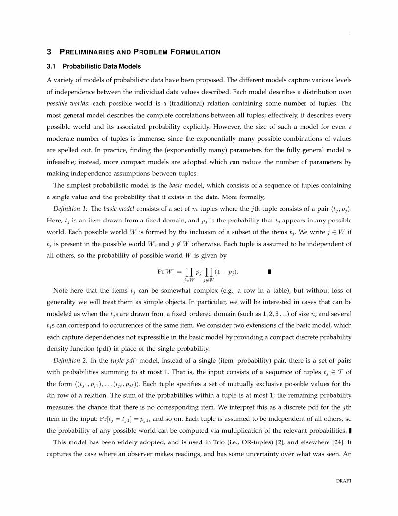
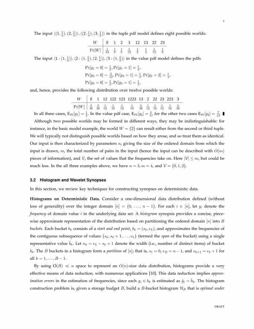
Example 1: Consider the ordered domain containing the three items 1, 2, 3. The input 〈1, 12 〉, 〈2, 1
3 〉, 〈2, 14 〉, 〈3, 1
2 〉
in the basic model defines the following twelve possible worlds and corresponding probabilities:
W ∅ 1 12 122 123 1223 13 2 22 23 223 3
Pr[W ] 18
18
548
148
548
148
18
548
148
548
148
18
DRAFT
7
The input 〈(1, 12 ), (2, 1
3 )〉, 〈(2, 14 ), (3, 1
2 )〉 in the tuple pdf model defines eight possible worlds:
W ∅ 1 2 3 12 13 22 23
Pr[W ] 124
18
18
112
18
14
112
16
The input 〈1 : (1, 12 )〉, 〈2 : (1, 1
3 ), (2, 14 )〉, 〈3 : (1, 1
2 )〉 in the value pdf model defines the pdfs
Pr[g1 = 0] = 12 ,Pr[g1 = 1] = 1
2 ,
Pr[g2 = 0] = 512 ,Pr[g2 = 1] = 1
3 ,Pr[g2 = 2] = 14 ,
Pr[g3 = 0] = 12 ,Pr[g3 = 1] = 1
2 ,
and, hence, provides the following distribution over twelve possible worlds:
W ∅ 1 12 122 123 1223 13 2 22 23 223 3
Pr[W ] 548
548
112
116
112
116
548
112
116
112
116
548
In all three cases, EW [g1] = 12 . In the value pdf case, EW [g2] = 5
6 , for the other two cases EW [g2] = 712 .
Although two possible worlds may be formed in different ways, they may be indistinguishable: for
instance, in the basic model example, the world W = 2 can result either from the second or third tuple.
We will typically not distinguish possible worlds based on how they arose, and so treat them as identical.
Our input is then characterized by parameters n, giving the size of the ordered domain from which the
input is drawn, m, the total number of pairs in the input (hence the input can be described with O(m)
pieces of information), and V , the set of values that the frequencies take on. Here |V| ≤ m, but could be
much less. In the all three examples above, we have n = 3,m = 4, and V = 0, 1, 2.
3.2 Histogram and Wavelet Synopses
In this section, we review key techniques for constructing synopses on deterministic data.
Histograms on Deterministic Data. Consider a one-dimensional data distribution defined (without
loss of generality) over the integer domain [n] = 0, . . . , n − 1. For each i ∈ [n], let gi denote the
frequency of domain value i in the underlying data set. A histogram synopsis provides a concise, piece-
wise approximate representation of the distribution based on partitioning the ordered domain [n] into B
buckets. Each bucket bk consists of a start and end point, bk = (sk, ek), and approximates the frequencies of
the contiguous subsequence of values sk, sk + 1, . . . , ek (termed the span of the bucket) using a single
representative value bk. Let nk = ek − sk + 1 denote the width (i.e., number of distinct items) of bucket
bk. The B buckets in a histogram form a partition of [n]; that is, s1 = 0, eB = n− 1, and sk+1 = ek + 1 for
all k = 1, . . . , B − 1.
By using O(B) n space to represent an O(n)-size data distribution, histograms provide a very
effective means of data reduction, with numerous applications [10]. This data reduction implies approx-
imation errors in the estimation of frequencies, since each gi ∈ bk is estimated as gi = bk. The histogram
construction problem is, given a storage budget B, build a B-bucket histogram HB that is optimal under
DRAFT
8
some aggregate error metric. The histogram error metrics to minimize include, for instance, the Sum-Squared-
Error
SSE(H) =n∑
i=1
(gi − gi)2 =B∑
k=1
ek∑i=sk
(gi − bk)2
(which defines the important class of V-optimal histograms [19], [21]) and the Sum-Squared-Relative-Error:
SSRE(H) =n∑
i=1
(gi − gi)2
maxc, |gi|2
(where constant c in the denominator avoids excessive emphasis being placed on small frequencies [11],
[14]). The Sum-Absolute-Error (SAE) and Sum-Absolute-Relative-Error (SARE) are defined similarly to SSE
and SSRE, replacing the square with an absolute value so that
SAE(H) =n∑
i=1
|gi − gi| ; SARE(H) =n∑
i=1
|gi − gi|maxc, |gi|
.
In addition to such cumulative metrics, maximum error metrics provide approximation guarantees on the
relative/absolute error of individual frequency approximations [14]; these include Maximum-Absolute-
Relative-Error
MARE(H) = maxi∈[n]
|gi − gi|maxc, |gi|
.
Histogram construction satisfies the principle of optimality: If the Bth bucket in the optimal histogram
spans the range [i + 1, n − 1], then the remaining B − 1 buckets must form an optimal histogram for
the range [0, i]. This immediately leads to a Dynamic-Programming (DP) algorithm for computing the
optimal error value OPTH[j, b] for a b-bucket histogram spanning the prefix [1, j] based on the following
recurrence:
OPTH[j, b]= min0≤l<j
h(OPTH[l, b− 1],minbBE([l + 1, j], b)), (2)
where BE([x, y], z) denotes the error contribution of a single histogram bucket spanning [x, y] using a
representative value of z to approximate all enclosed frequencies, and h(x, y) is simply x+y (respectively,
maxx, y) for cumulative (resp., maximum) error objectives. The key to translating the above recurrence
into a fast algorithm lies in being able to quickly find the best representative b and the corresponding
optimal error value BE() for the single-bucket case.
For example, in the case of the SSE objective the representative value minimizing a bucket’s SSE con-
tribution is exactly the average bucket frequency bk =Pek
i=skgi
nkgiving an optimal bucket SSE contribution
of:
minbk
BE(bk = [sk, ek], bk) =ek∑
i=sk
g2i −
1nk
( ek∑i=sk
gi
)2.
By precomputing two n-vectors that store the prefix sums∑j
i=0 gi and∑j
i=0 g2i for each j = 0, . . . , n− 1,
the SSE contribution for any bucket bk in the DP recurrence can be computed in O(1) time, giving rise
to an O(n2B) algorithm for building the SSE-optimal (or, V-optimal) B-bucket histogram [21]. Similar
DRAFT
9
l = 3 2 2
−1
1/2
g0 g1 g2 g3 g4 g5 g6 g7
c5
c0
c1 −5/4
0 2 3 5 4 4
−1
0
0 0c7c6
c3c2
c4
11/4
l = 1
l = 0
l = 2
+
−
+
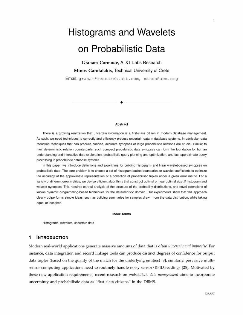
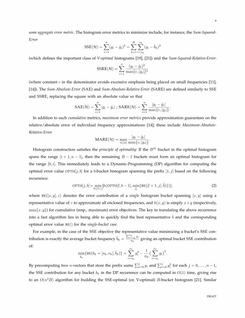
Fig. 1. Error-tree structure on n = 8 items for data distribution array A = [2, 2, 0, 2, 3, 5, 4, 4] (l = coefficient
resolution levels.)
ideas apply for the other error metrics discussed above. For instance, the optimal MARE contribution for
a single bucket depends only on the maximum/minimum frequencies. Using appropriate precomputed
data structures on dyadic ranges leads to an efficient, O(Bn log2 n) DP algorithm for building MARE-
optimal histograms on deterministic data [14].
Wavelets on Deterministic Data. Haar wavelet synopses [4], [12], [15], [33] provide another data reduction
tool based on the Haar Discrete Wavelet Decomposition (DWT) [31] for hierarchically decomposing
functions. At a high level, the Haar DWT of a data distribution over [n] consists of a coarse overall
approximation (the average of all frequencies) together with n− 1 detail coefficients (constructed through
recursive pairwise averaging and differencing) that influence the reconstruction of frequency values at
different scales. The Haar DWT process can be visualized through a binary coefficient tree structure, as in
Figure 1. Leaf nodes gi correspond to the original data distribution values in A[]. The root node c0 is the
overall average frequency, whereas each internal node ci (i = 1, . . . , 7) is a detail coefficient computed
as the half the difference between the average of frequencies in ci’s left child subtree and the average of
frequencies in ci’s right child subtree (e.g., c3 = 12 ( 3+5
2 − 4+42 ) = 0). Coefficients in level l are normalized
by a factor of√
2l: this makes the transform an orthonormal basis [31], so that the sum of squares of
coefficients equals the sum of squares of the original data values, by Parseval’s theorem.
Any data value gi can be reconstructed as a function of the coefficients which are proper ancestors
of the corresponding node in the coefficient tree: the reconstructed value can be found by summing
DRAFT
10
appropriately scaled multiples of these log N + 1 coefficients alone. For example, in Figure 1, g4 = c0 −
c1 + c6 = 114 − (− 5
4 )+ (−1) = 3. The support of a coefficient ci is defined as the interval of data values
that ci is used to reconstruct; it is a dyadic interval of size 2log n−l for a coefficient at resolution level l (see
Fig. 1).
Given limited space for maintaining a wavelet synopsis a thresholding procedure retains B n Haar coeffi-
cients as a highly-compressed approximate representation of the data (remaining coefficients are implicitly
set to 0). As with histogram construction, the aim is to determine the “best” subset of B coefficients to
retain, so that some overall error measure is minimized. By orthonormality of the normalized Haar basis,
greedily picking the B largest coefficients (based on absolute normalized value) is optimal for SSE error [31].
Recent work proposes schemes for optimal and approximate thresholding under different error metrics.
These schemes formulate a dynamic program over the coefficient-tree structure that tabulates the optimal
solution for a subtree rooted at node cj given the contribution from the choices made at proper-ancestor nodes
of cj in the tree. This idea handles a broad class of distributive error metrics (including all error measures
discussed above), as well as weighted Lp-norm error for arbitrary p) [12], [15].
There are two distinct versions of the thresholding problem for non-SSE error metrics. In the restricted
version the thresholding algorithm is forced to select values for the synopsis from the standard Haar
coefficient values (computed as discussed above). Such a restriction, however, may make little sense when
optimizing for non-SSE error, and can, in fact, lead to sub-optimal synopses for non-SSE error [15]. In
the unrestricted version of the problem, retained coefficient values are chosen to optimize the target error
metric [15]. Let OPTW[j, b, v] denote the optimal error contribution across all frequencies gi in the support
(i.e., subtree) of coefficient cj assuming a total space budget of b coefficients retained in cj ’s subtree; and,
a (partial) reconstructed value of v based on the choices made at proper ancestors of cj . Then, based on
the Haar DWT reconstruction process, we can compute OPTW[j, b, v] as the minimum of two alternative
error values at cj :
(1) Optimal error when retaining the best value for cj , found by minimizing over all values vj for cj and
allotments of the remaining budget across the left and right child of cj , i.e.,
OPTWr[j, b, v] = minvj ,0≤b′≤b−1
h(OPTW[2j, b′, v + vj ], OPTW[2j + 1, b−b′−1, v−vj ]).
(2) Optimal error when not retaining cj , computed similarly:
OPTWnr[j, b, v] = minvj ,0≤b′≤b
h(OPTW[2j, b′, v], OPTW[2j + 1, b− b′, v]),
where h() stands for summation (max) for cumulative (resp., maximum) error-metric objectives. In the
restricted problem, minimization over vj is eliminated (since the value for cj is fixed), and the values for
the “incoming” contribution v can be computed by stepping through all possible subsets of ancestors for
cj — since the depth of the tree is O(log n), this implies an O(n2) thresholding algorithm [12]. In the
unrestricted case, Guha and Harb propose efficient approximation schemes that employ techniques for
bounding and approximating the range of possible v values [15].
DRAFT
11
3.3 Probabilistic Data Reduction Problem
The key difference in the probabilistic data setting is that data-distribution frequencies gi (and the Haar
DWT coefficients) are now random variables. We use gi(W ) (ci(W )) to denote the (instantiated) frequency
of the ith item (resp., value of the ith Haar coefficient) in possible world W—we can omit the explicit
dependence on W for the sake of conciseness. The error of a given data synopsis is also a random variable
over the collection of possible worlds. Our goal becomes that of constructing a data synopsis (histogram
or wavelet) that optimizes an expected measure of the target error objective over possible worlds. More formally,
let err(gi, gi) denote the error of approximating gi by gi (e.g., squared error or absolute relative error for
item i); then, our problem can be formulated as follows.
[Synopsis Construction for Probabilistic Data] Given a collection of probabilistic attribute values, a
synopsis space budget B, and a target (cumulative or maximum) error metric, determine a histogram
synopsis with B buckets or a wavelet synopsis comprising B Haar coefficients that minimizes either (1)
the expected cumulative error over all possible worlds, i.e., EW [∑
i err(gi, gi)] (in the case of a cumulative
error objective); or, (2) the maximum value of the per-item expected error over all possible worlds, i.e.,
maxiEW [err(gi, gi)] (for a maximum error objective).
A natural first attempt to solve the probabilistic data reduction problem is to look to prior work, and
ask whether techniques based on sampling, or building a weighted deterministic data set could apply.
More precisely, one could try the Monte-Carlo approach of sampling a possible world W with probability
Pr[W ] and building the optimal synopsis for W (similar to [22]); or for each item i finding EW [gi], and
building the synopsis of the “expected” data. Our subsequent analysis shows that such attempts are
insufficient. We give precise formulations of the optimal solution to the problem under a variety of error
metrics, and one can verify by inspection that they do not in general correspond to any of these simple
solutions. Further, we compare the optimal solution to these solutions in our experimental evaluation,
and observe that the quality of the solution found is substantially poorer. This stands in contrast to prior
work on estimating functions such as expected number of distinct items [5], [24], which analyze the
number of samples needed to give an accurate estimate. This is largely because synopses are not scalar
values—it is not meaningful to find the “average” of multiple synopses.
4 HISTOGRAMS ON UNCERTAIN DATA
We first consider producing optimal histograms for probabilistic data under cumulative error objectives
which minimize the expected cost of the histogram over all possible worlds. Our techniques are based
on applying the dynamic programming approach. Most of our effort is in showing how to compute the
optimal b for a bucket b under a given error objective, and also to compute the corresponding value of
EW [BE(b, b)]. Here, we observe that the principle of optimality still holds even under uncertain data: since
the expectation of the sum of costs of each bucket is equal to the sum of the expectations, removing the
DRAFT
12
final bucket should leave an optimal B − 1 bucket histogram over the prefix of the domain. Hence, we
will be able to invoke equation (2), and find a solution which evaluates O(Bn2) possibilities.
4.1 Sum-squared error Histograms
The sum-squared error measure SSE is the sum of the squared differences between the values within
a bucket bk and the representative value of the bucket, bk. For a fixed possible world W , the optimal
value for bi is the mean of the frequencies gi in the bucket and the measure reduces to a multiple of
the sample variance of the values within the bucket. This holds true even under probabilistic data, as
we show below. For deterministic data, it is straightforward to quickly compute the (sample) variance
within a given bucket, and therefore use dynamic programming to select the optimum bucketing [21].
In order to use the DP approach on uncertain data, which specifies exponentially many possible worlds,
we must be able to efficiently compute the variance in a given bucket b specified by start point s and
end point e.
Fact 1: Under the sum-squared error measure, the cost is minimized by setting b = 1nb
EW [∑e
i=s gi] = b.
Proof: The cost of the bucket is
SSE(b, b) =EW [e∑
i=s
(gi − b)2] = EW [e∑
i=s
(gi − b + b− b)2]
=e∑
i=s
EW [(gi − b)2] + EW [2(b− b)(gi − b) + (b− b)2]
=e∑
i=s
(EW [g2i ] + EW [b2 − 2gib](b− b)2) + 2(b− b)(EW [
e∑i=s
(gi − b)])
=e∑
i=s
(EW [g2i ]− b2 + (b− b)2).
Since the last term is always positive, it is minimized by setting b = b.
We can then write SSE(b, b) as the combination of two terms:
SSE(b, b) =e∑
i=s
EW [g2i ]− 1
nbEW
[ e∑i=s
gi
]2. (3)
The first term is the expectation (over possible worlds) of the sum of squares of frequencies of each
item in the bucket. The second term can be interpreted as the square of the expected weight of the bucket,
scaled by the span of the bucket. We show how to compute each term efficiently in our different models.
Value pdf model. In the value pdf model, we have a distribution for each item i over frequency values
vj ∈ V giving Pr[gi = vj ]. By independence of the pdfs, we havee∑
i=s
EW [g2i ] =
e∑i=s
∑vj∈V
Pr[gi = vj ]v2j .
DRAFT
13
Meanwhile, for the second term, we can find
EW [e∑
i=s
gi] =e∑
i=s
∑vj∈V
Pr[gi = vj ]vj .
Combining these two expressions, we obtain:
SSE(b, b) =e∑
i=s
∑vj∈V
Pr[gi = vj ]v2j −
1nb
( e∑i=s
∑vj∈V
Pr[gi = vj ]vj
)2.
Tuple pdf model. In the tuple pdf case, things seem more involved, due to interactions between items
in the same tuple. As shown by equation (3), we need to compute EW [g2i ] and EW [(
∑i gi)]2. Let the set
of tuples in the input be T = tj, so each tuple has an associated pdf giving Pr[tj = i], from which we
can derive Pr[a ≤ tj ≤ b], the probability that the ith tuple in the input is falls between a and b in the
input domain.
EW [g2i ] = VarW [gi] + (EW [gi])2 =
∑tj∈T
Pr[tj = i](1− Pr[tj = i]) + (∑tj∈T
Pr[tj = i])2.
Here, we rely on the fact that variance of each gi is the sum of the variances arising from each tuple in
the input. Observe that although there are dependencies between particular items, these do not affect the
computation of the expectations for individual items, which can be then be summed to find the overall
answer. For the second term, we treat all items in the same bucket together as a single item and compute
its expected square by iterating over all tuples in the input T :
EW [e∑
i=s
gi]2 = (∑tj∈T
Pr[s ≤ tj ≤ e])2.
Combining these,
SSE(b, b) =e∑
i=s
∑tj∈T
Pr[tj = i](1− Pr[tj = i]) + (∑tj∈T
Pr[tj = i])2
− 1nb
(∑tj∈T
Pr[s ≤ tj ≤ e])2.
Efficient Computation. The above development shows how to find the cost of a specified bucket.
Computing the minimum cost histogram requires comparing the cost of many different choices of buckets.
As in the deterministic case, since the cost is the sum of the costs of the buckets, the dynamic programming
solution can find the optimal cost. This computes the cost of the optimal j bucket solution up to position
` combined with the cost of the optimal k−j bucket solution over positions `+1 to n. This means finding
the cost of O(n2) buckets. By analyzing the form of the above expressions for the cost of a bucket, we
can precompute enough information to allow the cost of any specified bucket to be found in time O(1).
DRAFT
14
For the tuple pdf model (the value pdf model is similar but simpler) we precompute arrays of length
n:
A[e] =e∑
i=1
( ∑tj∈T
Pr[tj = i](1− Pr[tj = i]) + (∑tj∈T
Pr[tj = i])2)
B[e] =∑tj∈T
Pr[tj ≤ e],
for 1 ≤ e ≤ s, and set A[0] = B[0] = 0. Then, the cost SSE((s, e), b) is given by
A[e]−A[s− 1]− (B[e]−B[s−1])2
(e−s+1) .
With the input in sorted order, these three arrays can be computed with a linear pass over the input.
In summary:
Theorem 1: Optimal SSE histograms can be computed over probabilistic data presented in the value
pdf or tuple pdf models in time O(m + Bn2).
4.2 Sum-Squared-Relative-Error Histograms
The sum of squares of relative errors measure, SSRE over deterministic data computes the difference
between b, the representative value for the bucket, and each value within the bucket, and reports the
square of this difference as a ratio to the square of the corresponding value. Typically, an additional
‘sanity’ parameter c is used to limit the value of this quantity in case some values in the bucket are very
small. With probabilistic data, we take the expected value of this quantity over all possible worlds. So,
given a bucket b, the cost is
SSRE(b, b) = EW
[e∑
i=s
(gi − b)2
max(c2, g2i )
].
By linearity of expectation, the cost given b can be computed by evaluating at all values of gi which have
a non-zero probability (i.e. at all v ∈ V).
Value pdf model. We write the SSRE cost in terms of the probability that, over all possible worlds, the
ith item has frequency vj ∈ V . Then,
SSRE(b, b) =e∑
i=s
∑vj∈V
Pr[gi = vj ](vj − b)2
max(c2, v2j )
. (4)
We rewrite this using the function w(x) = 1/ max(c2, x2), which is a fixed value once x is specified.
Now, our cost is
SSRE(b, b) =e∑
i=s
∑vj∈V
(Pr[gi = vj ]w(vj)v2
j
− 2 Pr[gi = vj ]w(vj)vj b + Pr[gi = vj ]w(vj)b2),
DRAFT
15
which is a quadratic in b. Simple calculus demonstrates that the optimal value of b to minimize this cost
is
b =
∑ei=s
∑vj∈V Pr[gi = vj ]vjw(vj)∑e
i=s
∑vj∈V Pr[gi = vj ]w(vj)
.
Substituting this value of b gives SSRE(b, b) =eX
i=s
Xvj∈V
Pr[gi = vj ]v2j w(vj)−
(Pe
i=s
Pvj∈V Pr[gi = vj ]vjw(vj))
2Pei=s
Pvj∈V Pr[gi = vj ]w(vj)
.
Define the following arrays:
X[e] =∑e
i=1
∑vj∈V Pr[gi = vj ]v2
j w(vj)
Y [e] =∑e
i=1
∑vj∈V Pr[gi = vj ]vjw(vj)
Z[e] =∑e
i=1
∑vj∈V Pr[gi = vj ]w(vj).
The cost of any bucket specified by s and e is found in constant time from these as:
minb
SSE((s, e), b) = X[e]−X[s− 1]− (Y [e]− Y [s− 1])2
Z[e]− Z[s− 1].
Dynamic programming then finds the optimal set of buckets. One can also verify that if we fix w(v) = 1
for all v, corresponding to the sum of squared errors, then after rearrangement and simplification, this
expression reduces to that in Section 4.1. It also solves the deterministic version of the problem in the
case where each value pdf gives certainty of achieving a particular frequency.
Tuple pdf model. For this cost measure, the cost for the bucket b given by equation (4) is the sum of
costs obtained by each item in the bucket. We can focus solely on the contribution to the cost made by a
single item i, and observe that equation (4) depends only on the (induced) distribution giving Pr[gi = vj ]:
there is no dependency on any other item. So we compute the induced value pdf (Section 3.1) for each
item independently, and apply the above analysis.
Theorem 2: Optimal SSRE histograms be can computed over probabilistic data presented in the value
pdf model in time O(m + Bn2) and O(m|V|+ Bn2) in the tuple pdf model.
4.3 Sum-Absolute-Error Histograms
Let V be the set of possible values taken on by the gis, indexed so that v1 ≤ v2 ≤ . . . ≤ v|V|. Given some
b, let j′ satisfy vj′ ≤ b < vj′+1 (we can insert ‘dummy’ values of v0 = 0 and v|V|+1 = ∞ if b falls outside
DRAFT
16
of v1 . . . v|V|). The sum of absolute errors is given by
SAE(b, b) =e∑
i=s
∑vj∈V
Pr[gi = vj ]|b− vj |
=e∑
i=s
(b− vj′) Pr[gi ≤ vj′ ] + (vj′+1 − b) Pr[gi ≥ vj′+1]
+∑vj∈V
Pr[gi ≤ vj ](vj+1 − vj) if vj < vj′
Pr[gi > vj ](vj+1 − vj) if vj ≥ vj′ .
The contribution of the first two terms can be written as
(vj′+1 − vj′) Pr[gi ≤ vj′ ] + (b− vj′+1)(Pr[gi ≤ vj′ ]− Pr[gi ≥ vj′+1]).
This gives a quantity that is independent of b added to one that depends linearly on Pr[gi ≤ vj′ ]−Pr[gi >
vj′+1], which we define as ∆j′ . So if ∆j′ > 0, we can reduce the cost by making b closer to vj′+1; if ∆j′ < 0,
we can reduce the cost by making b closer to vj′ . Therefore, the optimal value of b occurs when we make
it equal to some vj value (since, when ∆j′ = 0, we have the same result when setting b to either vj′ or
vj′+1, or anywhere in between). So, we assume that b = vj′ for some vj′ ∈ V and can state
SAE(b, b) =e∑
i=s
∑vj∈V
Pr[gi ≤ vj ](vj+1 − vj) if b > vj
Pr[gi > vj ](vj+1 − vj) if b ≤ vj .
Now, set
Pj,s,e =e∑
i=s
Pr[gi ≤ vj ] and P ∗j,s,e =
e∑i=s
Pr[gi > vj ].
Observe that Pj,s,e is monotone increasing in j while P ∗j,s,e is monotone decreasing in j. So, we have
SAE(b, b) =∑vj<b
Pj,s,e(vj+1 − vj) +∑vj≥b
(P ∗j,s,e)(vj+1 − vj). (5)
There is a contribution of (vj+1−vj) for all j values, multiplied by either P [j, s, e] or P ∗[j, s, e]. Consider
the effect on SAE if we step b through values v1, v2 . . . v|V|. We have
SAE(b, v`+1)− SAE(b, v`) = (P`,s,e − P ∗`+1,s,e)(v`+1 − v`).
Because Pj,s,e is monotone increasing in j, and P ∗j,s,e is monotone decreasing in j, the quantity P`,s,e −
P ∗`+1,s,e is monotone increasing in `. Thus SAE(b, b) can have a single minimum value as b is varied, and
is increasing in both directions away from this value. Importantly, this minimum does not depend on the
vj values themselves; instead, it occurs (approximately) when Pj,s,e ≈ P ∗j,s,e ≈ nb/2, where nb = (e−s+1)
as before. It therefore suffices to find the v′j value defined by
v′j = arg minv`∈V
∑vj<v`∈V
Pj,s,e +∑
vj>v`∈VP ∗
j,s,e,
and then set b = vj′ to obtain the optimal SAE cost.
DRAFT
17
Tuple and Value pdf models. In the value pdf case, it is straightforward to compute the P and P ∗ values
directly from the input pdfs. For the tuple pdf case, observe that from the form of the expression for
SAE, there are no interactions between different gi values: although the input specifies interactions and
(anti)correlations between different variables, for computing the error in a bucket we can treat each item
independently in turn. We therefore convert to the induced value pdf (at an additional cost of O(m|V|)),
and use this in our subsequent computations.
Efficient Computation. To quickly find the cost of a given bucket b, we first find the optimal b. We
precompute∑
vj<` Pj,1,e(vj+1 − vj) and∑
vj≥` P ∗j,1,e(vj+1 − vj) values for all v` ∈ V and e ∈ [n]. Now
SAE(b, b) for any b ∈ V can be computed (from (5)) as the sum of two differences of precomputed values.
The minimum value attainable by any b can then be found by a ternary search over the values V , using
O(log |V|) probes. Finally, the cost for the bucket using this b is also found from the same information.
The time cost is O(|V|n) preprocessing to build tables of prefix sums, and O(log |V|) to find the optimal
cost of a given bucket. Therefore,
Theorem 3: Optimal SAE histograms can be computed over probabilistic data presented in the (induced)
value pdf model in time O(n(|V|+ Bn + n log |V|)).
For all of models of probabilistic data, |V| ≤ m is polynomial in the size of the input, so the total cost
is also polynomial.
4.4 Sum-Absolute-Relative-Error Histograms
For sum of absolute relative errors, bucket cost SARE(b, b) is
EW(e∑
i=s
|gi − b|max(c, gi)
) =e∑
i=s
∑vj∈V
Pr[gi = vj ]max(c, vj)
|vj − b| =e∑
i=s
∑vj∈V
wi,j |vj − b|,
where we define wi,j = Pr[gi=vj ]max(c,vj)
. But, more generally, the wi,j can be arbitrary non-negative weights.
This expression is more complicated than the squared relative error version due to the absolute value in
the numerator. Setting j′ so that vj′ ≤ b ≤ vj′+1, we can write the cost as
e∑i=s
∑vj∈V
wi,j(b− vj) if vj < b
wi,j(vj − b) if vj ≥ b
=e∑
i=s
∑vj∈V
wi,j(b− vj′ +∑
vj≤v`<vj′ v`+1 − v`) if vj < b
wi,j(vj′ − b +∑
vj′≤v`<vjv`+1 − v`) if vj ≥ b.
(6)
We define Wi,j =∑j
r=1 wi,r and W ∗i,j =
∑|V |r=j+1 wi,r, so that, rearranging the previous sum, the cost is
SARE(b, b) =e∑
i=s
Wi,j′(b− vj′)−W ∗i,j(b− vj′+1) +
∑vj∈V
Wi,j(vj+1 − vj) for vj′ > vj
W ∗i,j(vj − vj−1) for vj′ ≤ vj .
DRAFT
18
The same style of argument as above suffices to show that the optimal choice of b is when b = vj′ for
some j′. We define Pj,s,e =∑e
i=s Wi,` and P ∗j,s,e =
∑ei=s W ∗
i,`, so we have
SARE(b, b) =∑
vj′>vj∈V
Pj,s,e(vj+1 − vj) +∑
vj′≤vj∈V
P ∗j,s,e(vj+1 − vj).
Observe that this matches the form of (5). As in Section 4.3, Pj,s,e is monotone increasing in j, and
P ∗j,s,e is decreasing in j. Therefore, the same argument holds to show that there is a unique minimum
value of SARE, and it can be found by a ternary search over the range. Likewise, the form of the cost in
equation (6) shows that there are no interactions between different items, so we work in the (induced)
value pdf model. By building corresponding data structures based on tabulating prefix sums of the new
P and P ∗ functions, we conclude:
Theorem 4: Optimal SARE histograms can be computed over probabilistic data presented in the tuple
and value pdf models in time O(n(|V|+ Bn + n log |V| log n)).
4.5 Max-Absolute-Error and Max-Absolute-Relative-Error
Thus far, we have relied on the linearity of expectation and related properties such as summability of
variance to simplify the expressions of cost and aid in the analysis. When we consider other error metrics,
such as the maximum error and maximum relative error, we cannot immediately use such linearity
properties, and so the task becomes more involved. Here, we provide results for maximum absolute
error and maximum absolute relative error, MAE and MARE. Over a deterministic input, the maximum
error in a bucket b is MAE(b, b) = maxs≤i≤e |gi − b|, and the maximum relative error is MARE(b, b) =
maxs≤i≤e|gi−b|
max(c,gi). We focus on bounding the maximum value of the per-item expected error1. Here, we
consider the frequency of each item in the bucket in turn for the expectation, and then take the maximum
over these costs. So, we can write the costs as
MAE(b, b) = maxs≤i≤e
∑vj∈V
Pr[gi = vj ]|vj − b|
MARE(b, b) = maxs≤i≤e
∑vj∈V
Pr[gi = vj ]max(c, vj)
|vj − b|.
We can represent these both as maxs≤i≤e
∑|V |j=1 wi,j |vj − b|, where wi,j are non-negative weights indepen-
dent of b. Now observe that we have the maximum over what can be thought of as nb parallel instances of
a sum-absolute relative error (SARE) problem, one for each i value. Following the analysis in Section 4.4,
we observe that each function fi(b) =∑|V|
j=1 |vj − b| has a single minimum value, and is increasing away
from its minimum. It follows that the upper envelope of these functions, given by maxs≤i≤e fi(b) also
has a single minimum value, and is increasing as we move away from this minimum. So we can perform
1. The alternate formulation, where we seek to minimize the expectation of the maximum error, is also plausible, and worthy of
further study.
DRAFT
19
a ternary search over the values of vj to find j′ such that the optimal b lies between vj′ and vj′+1. Each
evaluation for a chosen value of b can be completed in time O(nb): that is, O(1) for each value of i,
by creating the appropriate prefix sums as discussed in Section 4.4 (it is possible to improve this cost
by appropriate precomputations, but this will not significantly alter the asymptotic cost of the whole
operation). The ternary search over the values in V takes O(log |V|) evaluations, giving a total cost of
O(nb log |V|).
Knowing that b must lie in this range, the cost is of the form
MARE(b, b) = maxs≤i≤e
αi(b− vj′) + βi(vj′+1 − b) + γi = maxs≤i≤e
b(αi − βi) + (γi + βivj′+1 − αivj′),
where the αi, βi, γi values are determined solely by j′, the wi,j ’s and the vjs, and are independent of b.
This means we must now minimize the maximum value of a set of univariate linear functions in the
range vj′ ≤ b ≤ vj′+1. A divide-and-conquer approach, based on recursively finding the intersection of
convex hulls of subsets of the linear functions yields an O(nb log nb) time algorithm2. Combining these,
we determine that evaluating the optimal b and the corresponding cost for a given bucket takes time
O(nb log nb|V|). We can then apply the dynamic programming solution, since the principle of optimality
holds over this error objective. Because of the structure of the cost function, it suffices to move from the
tuple pdf model to the induced value pdf, and so we conclude,
Theorem 5: The optimal B bucket histogram under maximum-absolute-error (MAE) and maximum-
absolute-relative-error (MARE) over data in either the tuple or value pdf models can be found in time
O(n2(B + n log n|V|)).
5 HAAR WAVELETS ON PROBABILISTIC DATA
We first present our results on the core problem of finding the B term optimal wavelet representation
under sum-squared error, and then discuss extensions to other error objectives.
5.1 SSE-Optimal Wavelet Synopses
Any input defining a distribution over original gi values immediately implies a distribution over Haar
wavelet coefficients ci. Assume that we are already in the transformed Haar wavelet space; that is, we
have a possible-worlds distribution over Haar DWT coefficients, with ci(W ) denoting the instantiation
of ci in world W (defined by the gi(W )s). Our goal is to pick B coefficient indices I and corresponding
coefficient values ci for each i ∈ I to minimize the expected SSE in the data approximation. By Parseval’s
theorem [31] and linearity of the Haar transform in each possible world, the SSE of the data approximation
is the SSE in the approximation of the normalized wavelet coefficients. By linearity of expectation, the
2. The same underlying optimization problem arises in a weighted histogram context—see [17] for the full details.
DRAFT
20
expected SSE for the resulting synopsis Sw(I) is:
EW [SSE(Sw(I))] =∑i∈I
EW [(ci − ci)2] +∑i 6∈I
E[(ci)2].
Suppose we are to include i in our index set I of selected coefficients. Then, the optimal setting of ci is
the expected value of the ith (normalized) Haar wavelet coefficient, by the same argument style as Fact 1.
That is,
µci = EW [ci] =∑wj
Pr[ci = wj ] · wj ,
computed over the set of values taken on by the coefficients, wj . Further, by linearity of expectation and
the fact that the Haar wavelet transform can be thought of as a linear operator H applied to the input
vector A, we have
µci = EW [Hi(A)] = Hi(EW [A]).
In other words, we can find the µci ’s by computing the wavelet transform of the expected frequencies,
EW(gi). So, the µci’s can be computed with linear effort from the input, in either tuple pdf or value pdf
form. Based on the above observation, we can rewrite the expected SSE as:
EW [SSE(Sw(I))] =∑i∈I
σ2ci
+∑i 6∈I
E[(ci)2],
where σ2ci
= VarW [ci] is the variance of ci. From the above expression, it is clear that the optimal strategy is
to pick the B coefficients giving the largest reduction in the expected SSE (since there are no interactions
across coefficients); furthermore, the “benefit” of selecting coefficient i is exactly E[(ci)2]−σ2ci
= µ2ci
. Thus,
the thresholding scheme that optimizes expected SSE is to simply select the B Haar coefficients with
the largest (absolute) expected normalized value. (This scheme naturally generalizes the conventional
deterministic SSE thresholding case (Section 3.2).)
Theorem 6: With O(n) time and space, we can compute the optimal SSE wavelet representation of
probabilistic data in the tuple and value pdf models.
Example. Suppose again that we have a distribution on wavelet coefficients (1, 2, 3), defined by the tuples
(1, 12 ), (2, 1
3 ), (2, 14 ), (3, 1
2 ). 2 has the largest absolute mean, of 712 . Picking this as the k = 1 coefficient
representation incurs expected error σ21 + 1
212 + 1212 = 1 + 708
123 = 1.4097.
5.2 Wavelet Synopses for non-SSE Error
The DP recurrence formulated over the Haar coefficient error tree for non-SSE error metrics in the
deterministic case (Section 3.2) extends naturally to the case of probabilistic data. The only change is
that we now define OPTW[j, b, v] to denote the expected optimal value for the error metric of interest
under the same conditions as the deterministic case. The recursive computation steps remain exactly the
same. The interesting point with the coefficient-tree DP recurrence is that almost all of the actual error
DRAFT
21
computation takes place at the leaf (i.e., data) nodes of the tree — the DP recurrences combine these
computed error values appropriately in a bottom-up fashion. For deterministic data, the error at a leaf
node i with an incoming value of v from its parents is just the point error metric of interest with gi = v;
that is, for leaf i, we compute OPTW[i, 0, v] = err(gi, v) which can be done in O(1) time (note that leaf
entries in OPTW[] are only defined for b = 0 since space is never allocated to leaves).
In the case of probabilistic data, such leaf-error computations are a little more complicated since we
now need to compute the expected point-error value
EW [err(gi, v)] =∑W
Pr[W ] · err(gi(W ), v),
over all possible worlds W ∈ W . But this computation can still be done in O(1) time assuming pre-
computed data structures similar to those we have derived for error objectives in the histogram case. To
illustrate the main ideas, consider the case of absolute relative error metrics, i.e., err(gi, gi) = w(gi) · |gi− gi|
where w(gi) = 1/ maxc, |gi|. Then, we can expand the expected error at gi as follows:
OPTW[i, 0, v] = EW [w(gi) · |gi − v|] =∑vj∈V
Pr[gi = vj ]w(vj) ·
(v − vj) if v > vj
(vj − v) if v ≤ vj ,
where, as earlier, V denotes the set of possible values for any frequency random variable gi. So, we have
an instance of a sum-absolute-relative-error problem, since the form of this optimization matches that in
Section 4.3. By precomputing appropriate arrays of size O(|V|) for each i, we can search for the optimal
“split point” vj′ ∈ V in time O(log |V|).
We can do the above computation in O(log |V|) time by precomputing two O(n|V|) arrays A[i, x], B[i, x],
and two O(n) arrays C[i], D[i], defined as follows:
A[i, x] =∑v′≤x
Pr[gi = v′]w(v′) C[i] =∑v′
Pr[gi = v′]w(v′)
B[i, x] =∑v′≤x
Pr[gi = v′]v′w(v′) D[i] =∑v′
Pr[gi = v′]v′w(v′),
for all i ∈ [n] and all possible “split points” x ∈ V . Then, given an incoming contribution v from ancestor
nodes, we perform a logarithmic search to recover the largest value xv ∈ V such that xv ≤ v, and compute
the expected error as:
EW [w(gi) · |gi − v|] = v(2A[i, xv]− C[i]) + D[i]− 2B[i, xv].
The above precomputation ideas naturally extend to other error metrics as well, and allow us to
easily carry over the algorithms and results (modulo the small O(log |V|) factor above) for the restricted
case, where all coefficient values are fixed, e.g., to their expected values as required for expected SSE
minimization. The following theorem summarizes:
DRAFT
22
0
20
40
60
80
100
0 200 400 600 800 1000
Err
or
%
Buckets
Sum squared errror, n=104
ProbabilisticExpectation
Sampled World
(a) Squared error
0
20
40
60
80
100
0 200 400 600 800 1000
Err
or
%
Buckets
Sum of Absolute Error n=104
ProbabilisticExpectation
Sampled World
(b) Absolute error
0
200
400
600
800
1000
1200
0 200 400 600 800 1000
Tim
e / s
Buckets
Sum Squared Relative Error Time Cost, n=104
(c) Time as B varies
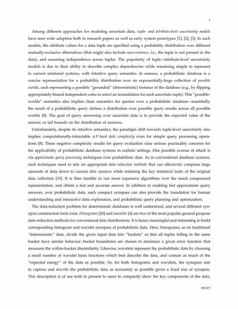
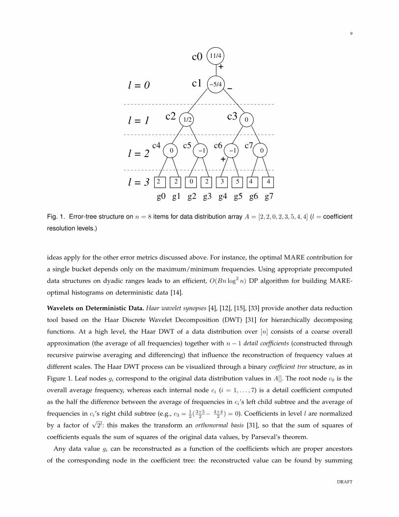
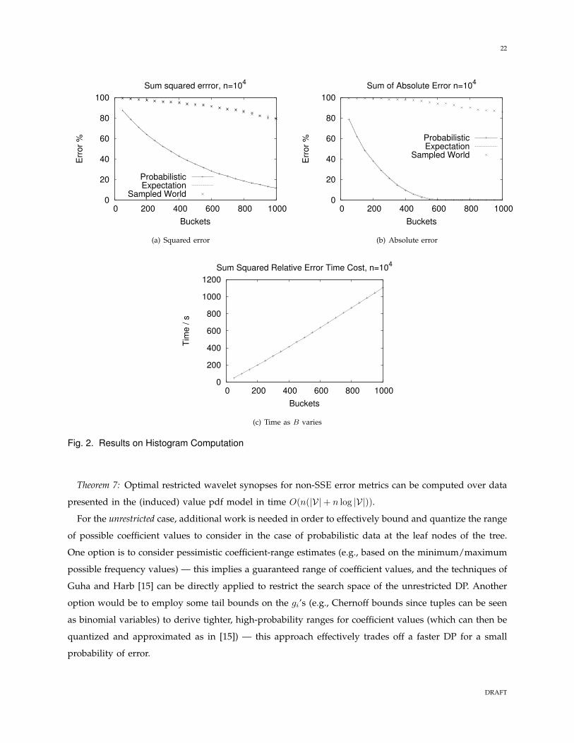
Fig. 2. Results on Histogram Computation
Theorem 7: Optimal restricted wavelet synopses for non-SSE error metrics can be computed over data
presented in the (induced) value pdf model in time O(n(|V|+ n log |V|)).
For the unrestricted case, additional work is needed in order to effectively bound and quantize the range
of possible coefficient values to consider in the case of probabilistic data at the leaf nodes of the tree.
One option is to consider pessimistic coefficient-range estimates (e.g., based on the minimum/maximum
possible frequency values) — this implies a guaranteed range of coefficient values, and the techniques of
Guha and Harb [15] can be directly applied to restrict the search space of the unrestricted DP. Another
option would be to employ some tail bounds on the gi’s (e.g., Chernoff bounds since tuples can be seen
as binomial variables) to derive tighter, high-probability ranges for coefficient values (which can then be
quantized and approximated as in [15]) — this approach effectively trades off a faster DP for a small
probability of error.
DRAFT
23
0
20
40
60
80
100
0 200 400 600 800 1000
Err
or
%
Buckets
Sum squared relative error, n=104, c=0.1
ProbabilisticExpectation
Sampled World
(a) Squared relative error with c = 0.1
0
20
40
60
80
100
0 200 400 600 800 1000
Err
or
%
Buckets
Sum squared relative error, n=104, c=0.5
ProbabilisticExpectation
Sampled World
(b) Squared relative error with c = 0.5
0
20
40
60
80
100
0 200 400 600 800 1000
Err
or
%
Buckets
Sum squared relative error, n=104, c=1.0
ProbabilisticExpectation
Sampled World
(c) Squared relative error with c = 1.0
0
20
40
60
80
100
0 200 400 600 800 1000
Err
or
%
Buckets
Sum of Relative Errors, n=104, c=0.1
ProbabilisticExpectation
Sampled World
(d) Relative error with c = 0.1
0
20
40
60
80
100
0 200 400 600 800 1000
Err
or
%
Buckets
Sum of Relative Errors, n=104, c=0.5
ProbabilisticExpectation
Sampled World
(e) Relative error with c = 0.5
0
20
40
60
80
100
0 200 400 600 800 1000
Err
or
%
Buckets
Sum of Relative Errors, n=104 c=1.0
ProbabilisticExpectation
Sampled World
(f) Relative error with c = 1.0
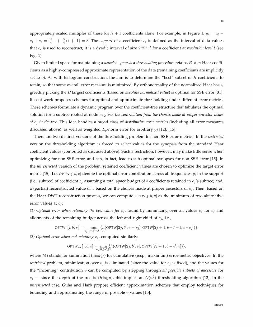
Fig. 3. Results on Histogram Computation with Relative Error
DRAFT
24
6 EXPERIMENTS
We implemented our algorithms in C, and carried out a set of experiments to compare the quality and
scalability of our results against those from naively applying methods designed for deterministic data.
Experiments were performed on a desktop 2.4GHz machine with 2GB RAM.
Data Sets. We experimented using a mixture of real and synthetic data sets. The real dataset came from
the MystiQ project3 which includes approximately m = 127, 000 tuples describing 27, 700 distinct items.
These correspond to links between a movie database and an e-commerce inventory, so the tuples for each
item define the distribution of the number of expected matches. This uncertain data provides input in the
basic model. Synthetic data was generated using the MayBMS [1] extension to the TPC-H generator 4. We
used the lineitem-partkey relation, where the multiple possibilities for each uncertain item are interpreted
as tuples with uniform probability over the set of values in the tuple pdf model.
Sampled Worlds and Expectation. We compare our methods to the two naive methods of building a
synopsis for uncertain data using deterministic techniques discussed in Section 3.3. The first is to simply
sample a possible world, and compute the (optimal) synopsis for this deterministic sample, as in [22]. The
second is to compute the expected frequency of each item, and build the synopsis of this deterministic
input. This can be thought of as equivalent to sampling many possible worlds, combining and scaling
the frequencies of these, and building the summary of the result. For consistency, we use the same code
to compute the respective synopses over both probabilistic and certain data, since deterministic data is
a special case of probabilistic data in the value pdf model.
6.1 Histograms on Probabilistic Data
We use our methods described in Section 4 to build the histogram over n items using B buckets, and
compute the cost of the histograms under the relevant metric (e.g. SSE, SARE, etc.). Observe that, unlike
in the deterministic case, a histogram with B = n buckets does not have zero error: we have to choose a
fixed representative b for each bucket, so any bucket with some uncertainty will have a contribution to
the expected cost. We therefore compute the percentage error of a given histogram as the fraction of the
cost difference between the one bucket histogram (largest achievable error) and the n bucket histogram
(smallest achievable error).
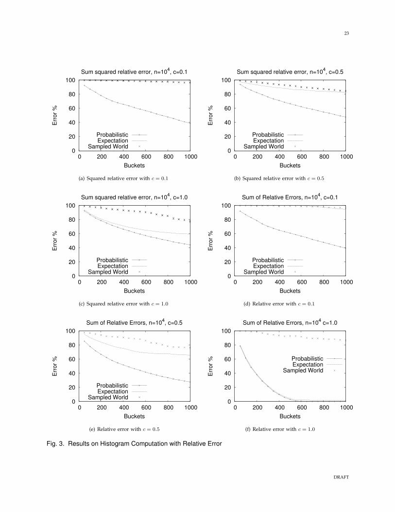
Quality. For uniformity, we show results for the MystiQ movie data set; results on synthetic data were
similar, and are omitted for brevity. The quality of the different methods on the same n = 10, 000 distinct
data items is shown in Figures 2 and 3. In each case, we measured the cost for using up to 1000 buckets
over the four cumulative error measures: SSE, SSRE, SAE, and SARE. We show two values of the sanity
3. http://www.cs.washington.edu/homes/suciu/project-mystiq.html
4. http://www.cs.cornell.edu/database/maybms/
DRAFT
25
0
200
400
600
800
1000
1200
1400
1600
0 5000 10000 15000 20000 25000 30000
Tim
e / s
n
Sum Squared Relative Error Time Cost, B=200
(a) Time as n varies
0
20
40
60
80
100
0 1000 2000 3000 4000 5000
Err
or
%
Coefficients
SSE Wavelets, Movie data, n=215
ProbabilisticSample
(b) Wavelets on real data
0
20
40
60
80
100
0 200 400 600 800 1000
Err
or
%
Coefficients
SSE Wavelets, Synthetic Data, n=215
ProbabilisticSample
(c) Wavelets on synthetic data
Fig. 4. Histogram timing costs and results on Wavelet Computation
constant for relative error, c = 0.5 and c = 1.0. Since our results show that the dynamic programming
finds the optimum set of buckets, there is no surprise that the cost is always smaller than the two naive
methods. Figure 3(b) shows a typical case for relative error: the probabilistic method is appreciably better
than using the expected costs, which in turn is somewhat better than building the histogram of a sampled
world. We show the results for three independent samples to show that there is fairly little variation in
the cost. For SSE and SAE (Figure 2(a) and 2(b)), while using a sampled world is still poor, the cost of
using the expectation is very close to that of our probabilistic method. The reason is that the histogram
obtains the most benefit by putting items with similar behavior in the same bucket, and on this data,
the expectation is a good indicator of behavioral similarity. This is not always the case, and indeed,
Figure 2(b) shows that while our method obtains the smallest possible error with about 600 buckets,
using the expectation never finds this solution. Other values of c tend to vary smoothly between two
DRAFT
26
extremes: increasing c allows the expectation method to get closer to the probabilistic solution (as in
Figure 3(f)). This is because as c approaches the maximum achievable frequency of any item, there is
no longer any dependency on the frequency, only on c, and so the cost function is essentially a scaled
version of the squared error or absolute error respectively. Reducing c towards 0 further disadvantages
the expectation method, and it has close to 100% error even when a very large number of buckets are
provided; meanwhile, the probabilistic method smoothly reduces in error down to zero.
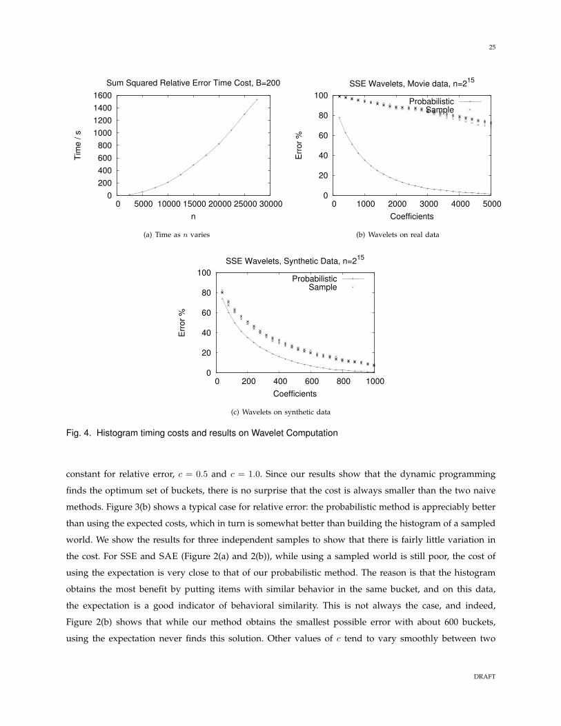
Scalability. Figures 2(c) and 4(a) show the time cost of our methods. We show the results for SSE,
although the results are very similar for other metrics, due to a shared code base. We see a strong linear
dependency on the number of buckets, B, and a close to quadratic dependency on n (since as n doubles,
the time cost slightly less than quadruples). This confirms our analysis that shows the cost is dominated
by an O(Bn2) term. The time to apply the naive methods is almost identical, since they both ultimately
rely on solving a dynamic program of the same size, which dwarfs any reduced linear preprocessing
cost. Therefore, the cost is essentially the same as for deterministic data. The time cost is acceptable, but
it suggests that for larger relations it will be advantageous to pursue the faster approximate solutions
outlined in Section 7.2.
6.2 Wavelets on Probabilistic Data
We implemented our methods for computing wavelets under the SSE objective. Here, the analysis shows
that the optimal solution is to compute the wavelet representation of the expected data (since this is
equivalent to generating the expected values of the coefficients, due to linearity of the wavelet transform
function), and then pick the B largest coefficients. We contrast to the effect of sampling possible worlds
and picking the coefficients corresponding to the largest coefficients of the sampled data. We measure the
error by computing the sum of the square of the µci ’s not picked by the method, and expressing this as a
percentage of the sum of all such µci’s, since our analysis demonstrates that this is the range of possible
error (Section 5.1). Figures 4(b) and 4(c) shows the effect of varying the number of coefficients B on the
real and synthetic data sets: while increasing the number of coefficients improves the cost in the sampled
case, it is much more expensive than the optimal solution. Both approaches take the same amount of
time, since they rely on computing a standard Haar wavelet transform of certain deterministic data: it
takes linear time to produce the expected values and then compute the coefficients; these are sorted to
find the B largest. This took much less than a second on our experimental set up.
7 EXTENSIONS
7.1 Multi-Dimensional Histograms
In this paper, we primarily consider summarizing one-dimensional probabilistic relations, since even
these can be sufficiently large to merit summarization. But, probabilistic databases can also contain rela-
tions which are multi-dimensional: these capture information about the correlation between the uncertain
DRAFT
27
attribute and multiple data dimensions. The description of such relations are naturally even larger, and
so even more deserving of summarization.
Our one-dimensional data can be thought of as defining a conditional distribution: given a value i,
we have a random variable X whose distribution is conditioned on i. Extending this to more complex
data, we have a random variable X whose distribution is conditioned on d other values: i, j, k . . .. This
naturally presents us with a multi-dimensional setting. In one dimension we argued that the typical case
is that similar values of i lead to similar distributions, which can be grouped together and replaced with
a single representative Similarly, the assumption is that similar regions in the multi-dimensional space
will have similar distributions, and so can be replaced by a common representative. Now, instead of
ranges of pdfs, the buckets will correspond to axis-aligned (hyper)rectangles in d-dimensional space.
More formally, in this setting each tuple tj is drawn from the cross-product of d ordered domains.
Without loss of generality, these can be thought of as defining d dimensional arrays, where each entry
consists of a probability distribution describing the behavior of the corresponding item. The goal is then to
partition this array into B (hyper)rectangles, and to retain a single representative of each (hyper)rectangle.
Our primary results above translate to this situation: given a (hyper)rectangle of pdfs, the optimal
representative for each error metric obeys the same properties. The intuition behind this is that while
the choice of a bucket depends on the ordered dimensions, the error within a bucket (and, hence, the
optimal representative) depends only on the set of pdfs which are within the bucket. For example, the
optimal representative for SSE is still the mean value of all the pdfs in the bucket. However, due to the
layout of the data, employing dynamic programming becomes more costly: firstly, because the dynamic
program has to consider a greater space of possible partitionings, and, secondly, because it may be more
difficult to quickly find the representative of a given (hyper)rectangle.
Consider the case of two-dimensional data under SSE. To find the cost of any given rectangular bucket,
we need to find the cost as given by (3). For the one-dimensional case, this can be done in constant time
by writing this expression as a function of a small number of terms, each of which can be computed for
the bucket based on prefix sums. The same concept applies in two-dimensions: given a bucket defined
by (s1, e1, s2, e2), we can find the sum of probabilities within the bucket in the tuple pdf model (say) by
precomputing B[e1, e2] =∑
tj∈T Pr[tj ∈ (0, e1, 0, e2)], i.e. the sum of probabilities that tuples fall in the
rectangle (0, e1, 0, e2). Then, the sum of probabilities for only the bucket is given by∑tj∈T
Pr[tj ∈ (s1, e1, s2, e2)] = B[e1, e2]−B[e1, s2 − 1]−B[s1 − 1, e2] + B[s1 − 1, s2 − 1].
Similar calculations follow naturally for other quantities (these are spelled out in detail in [18]). The
same principle extends to higher dimensions for finding the sum of values within any axis-aligned
(hyper)rectangle by evaluating an expression of 2d terms based on the Inclusion-Exclusion Principle (the
above case illustrates this for d = 2). This requires precomputing and storing a number of sums that is
linear in the size of the multi-dimensional domain.
DRAFT
28
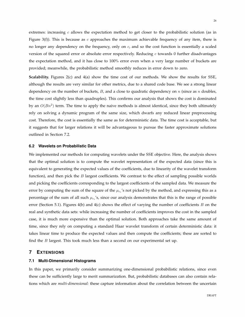
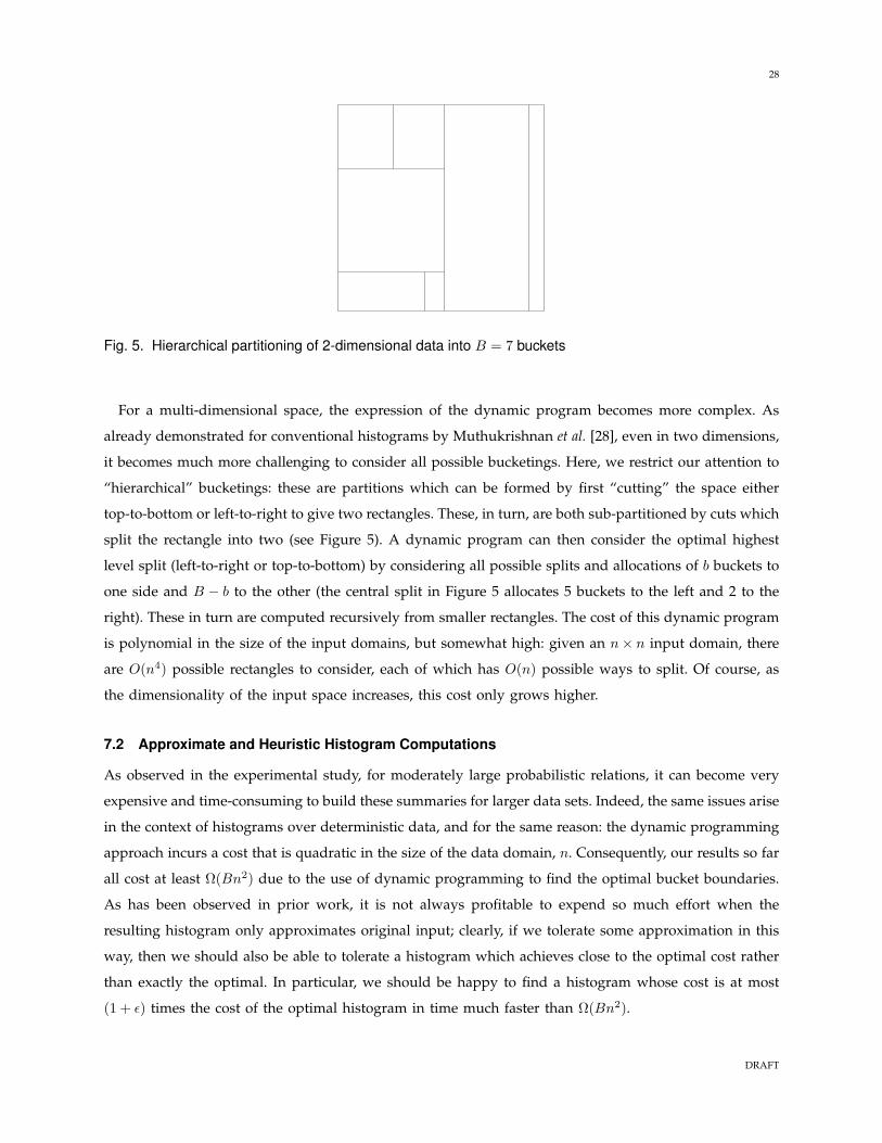
Fig. 5. Hierarchical partitioning of 2-dimensional data into B = 7 buckets
For a multi-dimensional space, the expression of the dynamic program becomes more complex. As
already demonstrated for conventional histograms by Muthukrishnan et al. [28], even in two dimensions,
it becomes much more challenging to consider all possible bucketings. Here, we restrict our attention to
“hierarchical” bucketings: these are partitions which can be formed by first “cutting” the space either
top-to-bottom or left-to-right to give two rectangles. These, in turn, are both sub-partitioned by cuts which
split the rectangle into two (see Figure 5). A dynamic program can then consider the optimal highest
level split (left-to-right or top-to-bottom) by considering all possible splits and allocations of b buckets to
one side and B − b to the other (the central split in Figure 5 allocates 5 buckets to the left and 2 to the
right). These in turn are computed recursively from smaller rectangles. The cost of this dynamic program
is polynomial in the size of the input domains, but somewhat high: given an n× n input domain, there
are O(n4) possible rectangles to consider, each of which has O(n) possible ways to split. Of course, as
the dimensionality of the input space increases, this cost only grows higher.
7.2 Approximate and Heuristic Histogram Computations
As observed in the experimental study, for moderately large probabilistic relations, it can become very
expensive and time-consuming to build these summaries for larger data sets. Indeed, the same issues arise
in the context of histograms over deterministic data, and for the same reason: the dynamic programming
approach incurs a cost that is quadratic in the size of the data domain, n. Consequently, our results so far
all cost at least Ω(Bn2) due to the use of dynamic programming to find the optimal bucket boundaries.
As has been observed in prior work, it is not always profitable to expend so much effort when the
resulting histogram only approximates original input; clearly, if we tolerate some approximation in this
way, then we should also be able to tolerate a histogram which achieves close to the optimal cost rather
than exactly the optimal. In particular, we should be happy to find a histogram whose cost is at most
(1 + ε) times the cost of the optimal histogram in time much faster than Ω(Bn2).
DRAFT
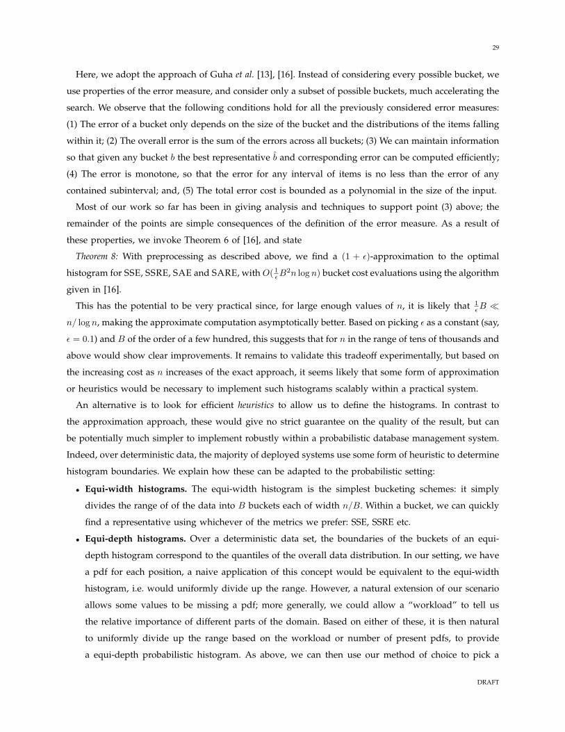
29
Here, we adopt the approach of Guha et al. [13], [16]. Instead of considering every possible bucket, we
use properties of the error measure, and consider only a subset of possible buckets, much accelerating the
search. We observe that the following conditions hold for all the previously considered error measures:
(1) The error of a bucket only depends on the size of the bucket and the distributions of the items falling
within it; (2) The overall error is the sum of the errors across all buckets; (3) We can maintain information
so that given any bucket b the best representative b and corresponding error can be computed efficiently;
(4) The error is monotone, so that the error for any interval of items is no less than the error of any
contained subinterval; and, (5) The total error cost is bounded as a polynomial in the size of the input.
Most of our work so far has been in giving analysis and techniques to support point (3) above; the
remainder of the points are simple consequences of the definition of the error measure. As a result of
these properties, we invoke Theorem 6 of [16], and state
Theorem 8: With preprocessing as described above, we find a (1 + ε)-approximation to the optimal
histogram for SSE, SSRE, SAE and SARE, with O( 1ε B2n log n) bucket cost evaluations using the algorithm
given in [16].
This has the potential to be very practical since, for large enough values of n, it is likely that 1ε B
n/ log n, making the approximate computation asymptotically better. Based on picking ε as a constant (say,
ε = 0.1) and B of the order of a few hundred, this suggests that for n in the range of tens of thousands and
above would show clear improvements. It remains to validate this tradeoff experimentally, but based on
the increasing cost as n increases of the exact approach, it seems likely that some form of approximation
or heuristics would be necessary to implement such histograms scalably within a practical system.
An alternative is to look for efficient heuristics to allow us to define the histograms. In contrast to
the approximation approach, these would give no strict guarantee on the quality of the result, but can
be potentially much simpler to implement robustly within a probabilistic database management system.
Indeed, over deterministic data, the majority of deployed systems use some form of heuristic to determine
histogram boundaries. We explain how these can be adapted to the probabilistic setting:
• Equi-width histograms. The equi-width histogram is the simplest bucketing schemes: it simply
divides the range of of the data into B buckets each of width n/B. Within a bucket, we can quickly
find a representative using whichever of the metrics we prefer: SSE, SSRE etc.
• Equi-depth histograms. Over a deterministic data set, the boundaries of the buckets of an equi-
depth histogram correspond to the quantiles of the overall data distribution. In our setting, we have
a pdf for each position, a naive application of this concept would be equivalent to the equi-width
histogram, i.e. would uniformly divide up the range. However, a natural extension of our scenario
allows some values to be missing a pdf; more generally, we could allow a “workload” to tell us
the relative importance of different parts of the domain. Based on either of these, it is then natural
to uniformly divide up the range based on the workload or number of present pdfs, to provide
a equi-depth probabilistic histogram. As above, we can then use our method of choice to pick a
DRAFT
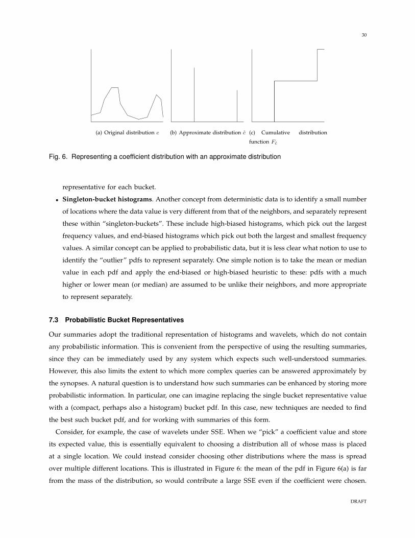
30
(a) Original distribution c (b) Approximate distribution c (c) Cumulative distribution
function Fc
Fig. 6. Representing a coefficient distribution with an approximate distribution
representative for each bucket.
• Singleton-bucket histograms. Another concept from deterministic data is to identify a small number
of locations where the data value is very different from that of the neighbors, and separately represent
these within “singleton-buckets”. These include high-biased histograms, which pick out the largest
frequency values, and end-biased histograms which pick out both the largest and smallest frequency
values. A similar concept can be applied to probabilistic data, but it is less clear what notion to use to
identify the “outlier” pdfs to represent separately. One simple notion is to take the mean or median
value in each pdf and apply the end-biased or high-biased heuristic to these: pdfs with a much
higher or lower mean (or median) are assumed to be unlike their neighbors, and more appropriate
to represent separately.
7.3 Probabilistic Bucket Representatives
Our summaries adopt the traditional representation of histograms and wavelets, which do not contain
any probabilistic information. This is convenient from the perspective of using the resulting summaries,
since they can be immediately used by any system which expects such well-understood summaries.
However, this also limits the extent to which more complex queries can be answered approximately by
the synopses. A natural question is to understand how such summaries can be enhanced by storing more
probabilistic information. In particular, one can imagine replacing the single bucket representative value
with a (compact, perhaps also a histogram) bucket pdf. In this case, new techniques are needed to find
the best such bucket pdf, and for working with summaries of this form.
Consider, for example, the case of wavelets under SSE. When we “pick” a coefficient value and store
its expected value, this is essentially equivalent to choosing a distribution all of whose mass is placed
at a single location. We could instead consider choosing other distributions where the mass is spread
over multiple different locations. This is illustrated in Figure 6: the mean of the pdf in Figure 6(a) is far
from the mass of the distribution, so would contribute a large SSE even if the coefficient were chosen.
DRAFT
31
Suppose we choose to represent the ith coefficient with an (approximate) pdf ci which indicates that
Pr[ci = vj ] = pj for some set of k values vj . For example, Figure 6(b) shows an approximate pdf c that
better captures the shape of Figure 6(a). We can denote the cumulative distribution function (cdf) of c as
Fc, and similarly for c as Fc. For the sum squared error in this setting, we obtain
EW [(ci − ci)2] =∑
x
Pr[c = x](x− F−1c (Fc(x)))2
That is, the cost of moving probability mass Pr[c = x] from x to where it is represented by c, which is
given by F−1c (Fc(x)). This generalizes the previous case where all the mass was placed at a single location
c: there, the implicit cdf was such that F−1c (p) = c for all probabilities p. Figure 6(c) shows that the cdf
of the approximate distribution in Figure 6(b). This definition can also be thought of as a special case
of the “Earth Mover’s Distance”, which measures the cost of moving probability mass within a metric
space. This distance has been used widely in comparing distributions over an ordered domain, and is
the natural extension of SSE to the case of a summarizing pdf [30], [27].
To optimize this error measure, observe that if we set v1 so that Pr[c = v1] = p1 for a particular p1
and try to choose the best v1, the optimal v1 is given by v1 =∑
v:Fc(v)≤p1Pr[c = v]v/p1, i.e. the weighted
average of the first p1 mass of probability from the distribution c (this is a natural generalization of Fact
1). Having found the optimal first representative, we can then “remove” the first p1 of probability mass
from c and continue on the remainder. This approach naturally lends itself to a dynamic programming
solution to find the optimal B term representation of a single coefficient c, where the choice is made over
the total probability mass allocated to the first b terms. The cost of this can be bounded by observing
that we only need consider probability values which occur within the distribution c, i.e. only over the
(discrete) values of F (c). Since c itself is formed from the Haar wavelet transform of the input, there
are at most O(|V| log n) such values. Hence, the dynamic programming can find these costs for a single
coefficient in time O(B|V| log n).
However, our goal is to find the optimal wavelet representation of all coefficients. Again, we can turn
to dynamic programming over the number of terms allocated, b, to summarize the first i coefficients
while minimizing the sum squared error. To do this, we first carry out the above dynamic programming
for all coefficients, and then consider allocating 0 . . . B terms to represent the ith coefficient in turn.
Accordingly, the total time to find the best probabilistic wavelet representation with a total of B terms
is O(Bn|V| log n + B2n).
The case for finding optimal histograms with pdfs to represent the buckets adds similar new challenges.
Some recent results in this direction are documented in [6].
8 CONCLUDING REMARKS
We have introduced the probabilistic data reduction problem, and given results for a variety of cumulative
and maximum error objectives, for both histograms and wavelets. Empirically, we see that the optimal
DRAFT
32
synopses can accurately summarize the data and are significantly better than simple heuristics. It remains
to better understand how to approximately represent and process probabilistic data, and to extend our
results to even more expressive models. So far, we have focused on the foundational one-dimensional
problem, but is also important to study multi-dimensional generalizations in greater detail. The error
objective formulations we have analyzed implicitly assume uniform workloads for point queries, and
so it remains to address the case when in addition to a distribution over the input data, there is also a
distribution over the queries to be answered.
Another direction for further research is in modeling and summarizing data which contains correlations
between tuples. Our work so far has assumed tuple independence: the input data treats all tuples (in the
tuple pdf model) or frequencies (in the value pdf model) as independent random variables. In some
situations, there are non-trivial correlations between tuples, which are not captured by these models.
One example of a more complex model which captures tuple dependencies is a Markov model where
the probability distribution of tuple depends on a recent history of previous tuples—for example, for
time-based data, the probability of the next tuple is conditioned on a constant number of the d most
recent tuples preceding it [26]. It is certainly possible to extend the approaches advocated here for more
compactly representing this data: we can think of each of the d values that the distribution depends on
as defining a point in d-dimensional space. If we can assume that the distributions conditioned on points
that are close in this space are similar, then we can apply the histogramming approach to more compactly
represent the full description of the distribution. However, this still leaves open the question of accurately
answering queries over such data: now, queries may be of the form “given an initial marginal distribution,
approximate the distribution n steps in the future” or, “given a current distribution, approximate the
probability that a certain event (or sequence of events) happened within the last n steps” [26]. For such
queries, new approaches to answering are needed, which may require new summarization methods.
Acknowledgments
We thank Sudipto Guha for some useful suggestions; Dan Suciu for the MystiQ data, and Dan Olteanu
for synthetic data from the MayBMS system.
DRAFT
33
REFERENCES
[1] L. Antova, T. Jansen, C. Koch, and D. Olteanu, “Fast and simple relational processing of uncertain data,” in IEEE International
Conference on Data Engineering, 2008.
[2] O. Benjelloun, A. D. Sarma, C. Hayworth, and J. Widomn, “An introduction to ULDBs and the Trio system,” IEEE Data
Engineering Bulletin, vol. 29, no. 1, pp. 5–16, Mar. 2006.
[3] J. Boulos, N. Dalvi, B. Mandhani, S. Mathur, C. Re, and D. Suciu, “Mystiq: A system for finding more answers by using
probabilities,” in ACM SIGMOD International Conference on Management of Data, 2005.
[4] K. Chakrabarti, M. Garofalakis, R. Rastogi, and K. Shim, “Approximate query processing using wavelets,” in International
Conference on Very Large Data Bases, 2000.
[5] G. Cormode and M. Garofalakis, “Sketching probabilistic data streams,” in ACM SIGMOD International Conference on
Management of Data, 2007.
[6] G. Cormode, A. Deligiannakis, M. Garofalakis, and A. McGregor, “Probabilistic histograms for probabilistic data,” in
International Conference on Very Large Data Bases, 2009.
[7] G. Cormode and A. McGregor, “Approximation algorithms for clustering uncertain data,” in ACM Principles of Database Systems,
2008.
[8] N. Dalvi and D. Suciu, “Efficient query evaluation on probabilistic databases,” in International Conference on Very Large Data
Bases, 2004.
[9] N. N. Dalvi and D. Suciu, “Management of probabilistic data: foundations and challenges,” in ACM Principles of Database
Systems, 2007.
[10] M. Garofalakis and P. B. Gibbons, “Approximate query processing: Taming the terabytes,” in International Conference on Very
Large Data Bases, 2001.
[11] ——, “Probabilistic wavelet synopses,” ACM Transactions on Database Systems, vol. 29, no. 1, Mar. 2004.
[12] M. Garofalakis and A. Kumar, “Wavelet synopses for general error metrics,” ACM Transactions on Database Systems, vol. 30,
no. 4, Dec. 2005.
[13] S. Guha, N. Koudas, and K. Shim, “Data streams and histograms,” in ACM Symposium on Theory of Computing, 2001, pp.
471–475.
[14] S. Guha, K. Shim, and J. Woo, “REHIST: Relative error histogram construction algorithms,” in International Conference on Very
Large Data Bases, 2004.
[15] S. Guha and B. Harb, “Wavelet synopsis for data streams: minimizing non-euclidean error,” in ACM SIGKDD, 2005.
[16] S. Guha, N. Koudas, and K. Shim, “Approximation and streaming algorithms for histogram construction problems,” ACM
Transactions on Database Systems, vol. 31, no. 1, pp. 396–438, 2006.
[17] S. Guha and K. Shim, “A note on linear time algorithms for maximum error histograms,” IEEE Transactions on Knowledge and
Data Engineering, vol. 19, no. 7, pp. 993–997, 2007.
[18] C.-T. Ho, R. Agrawal, N. Megiddo, and R. Srikant, “Range queries in olap data cubes,” in ACM SIGMOD International Conference
on Management of Data, 1997.
[19] Y. E. Ioannidis and V. Poosala, “Balancing histogram optimality and practicality for query result size estimation,” in ACM
SIGMOD International Conference on Management of Data, 1995, pp. 233–244.
[20] Y. E. Ioannidis, “The history of histograms (abridged),” in International Conference on Very Large Data Bases, 2003.
[21] H. V. Jagadish, N. Koudas, S. Muthukrishnan, V. Poosala, K. Sevcik, and T. Suel, “Optimal histograms with quality guarantees,”
in International Conference on Very Large Data Bases, 1998.
[22] R. Jampani, L. L. Perez, F. Xu, C. Jermaine, M. Wi, and P. Haas, “MCDB: A monte carlo approach to managing uncertain
data,” in ACM SIGMOD International Conference on Management of Data, 2008.
[23] T. S. Jayram, S. Kale, and E. Vee, “Efficient aggregation algorithms for probabilistic data,” in ACM-SIAM Symposium on Discrete
Algorithms, 2007.
[24] T. S. Jayram, A. McGregor, S. Muthukrishnan, and E. Vee, “Estimating statistical aggregates on probabilistic data streams,” in
ACM Principles of Database Systems, 2007.
DRAFT
34
[25] N. Khoussainova, M. Balazinska, and D. Suciu, “Towards correcting input data errors probabilistically using integrity
constraints,” in ACM Workshop on Data Engineering for Wireless and Mobile Access (MobiDE), 2006.
[26] J. Letchner, C. Re, M. Balazinska, and M. Philipose, “Access methods for markovian streams,” in IEEE International Conference
on Data Engineering, 2009.
[27] E. Levina and P. Bickel, “The earth mover’s distance is the mallows distance: some insights from statistics,” in IEEE International
Converence on Computer Vision, 2001.
[28] S. Muthukrishnan, V. Poosala, and T. Suel, “On rectangular partitionings in two dimensions: Algorithms, complexity, and
applications,” in International Conference on Database Theory, 1999, pp. 236–256.
[29] C. Re and D. Suciu, “Approximate lineage for probabilistic databases,” in International Conference on Very Large Data Bases,
2008.
[30] Y. Rubner, C. Tomasi, and L. J. Guibas, “A metric for distributions with applications to image databases,” in IEEE International
Conference on Computer Vision, 1998.
[31] E. J. Stollnitz, T. D. DeRose, and D. H. Salesin, “Wavelets for Computer Graphics – Theory and Applications”. San Francisco, CA:
Morgan Kaufmann Publishers, 1996.
[32] D. Suciu and N. N. Dalvi, “Foundations of probabilistic answers to queries,” in ACM SIGMOD International Conference on
Management of Data, 2005.
[33] J. S. Vitter and M. Wang, “Approximate computation of multidimensional aggregates of sparse data using wavelets,” in ACM
SIGMOD International Conference on Management of Data, 1999.
[34] Q. Zhang, F. Li, and K. Yi, “Finding frequent items in probabilistic data,” in ACM SIGMOD International Conference on
Management of Data, 2008.
[35] X. Zheng, “Topics in massive data summarization,” Ph.D. dissertation, University of Michigan, Aug. 2008.
Graham Cormode is a Principal Member of Technical Staff in the Database Research Department at AT&T
Labs-Research. His Ph.D. is from the University of Warwick, and he completed postdoctoral studies at the DI-
MACS Center in Rutgers University. He works on data stream algorithms, large-scale data mining, and applied
algorithms, with applications to databases, networks, and fundamentals of communications and computation.
Minos Garofalakis is a Professor of Computer Science at the Electronic and Computer Engineering (ECE)
Department of the Technical University of Crete (TUC), and the Director of the Software Technology and
Network Applications Lab (SoftNet) at TUC. He received the MSc and PhD degrees in Computer Science from
the Univ. of Wisconsin-Madison in 1994 and 1998, respectively. He has worked as a Member of Technical Staff
at Bell Labs, Lucent Technologies (1998-2005), as a Senior Researcher at Intel Research Berkeley (2005-
2007), and as a Principal Research Scientist at Yahoo! Research (2007-2008). In parallel, he also held an
Adjunct Associate Professor position at the EECS Dept. of the Univ. of California, Berkeley (2006-2008). He
currently serves as an Associate Editor for ACM Trans. on Database Systems (ACM TODS) and IEEE Trans. on Knowledge and
Data Engineering (IEEE TKDE), and as an Editorial Board Member for Foundations and Trends in Databases and the Proceedings
of the VLDB Endowment (PVLDB). He was the Core Database Technology PC Chair for VLDB’2007, and recently completed a term
as an Associate Editor for the IEEE Data Engineering Bulletin (2004-2006). His current research interests include data streaming,
probabilistic databases, approximate query processing, network-data management, and cloud databases.
DRAFT