Embed Size (px)
Citation preview

1
Hierarchical Tag visualization and application for tag recommendations
CIKM’11Advisor: Jia Ling, KohSpeaker: SHENG HONG, CHUNG

2
Outline
• Introduction• Approach– Global tag ranking
• Information-theoretic tag ranking• Learning-to-rank based tag ranking
– Constructing tag hierarchy• Tree initialization• Iterative tag insertion• Optimal position selection
• Applications to tag recommendation• Experiment

3
Introduction
BlogBlogtag
tag
tag
4
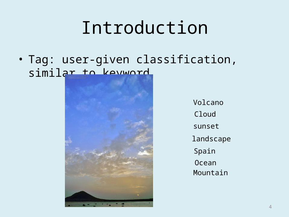
Introduction
• Tag: user-given classification, similar to keyword
Volcano
Cloud
sunset
landscape
Spain
OceanMountain

5
• Tag visualization– Tag cloud
Introduction
Volcano
Cloud
sunset
landscape
SpainOcean
Mountain
SpainCloud landscape
Mountain
Tag cloud

6
??
Which tags are abstractness?
Ex Programming->Java->j2ee

7

8
Approach
funny
newsdownload
nfl
nba
reviewslinks
sports
football education
image htmlbusiness
basketball
learning
image
sports funny reviews news
nfl
football
nba
basketball
htmldownload
links
learning business
education

9
Approach
• Global tag rankingimage
sports funny reviews news
nfl
football
nba
basketball
htmldownload
links
learning business
education
ImageSportsFunnyReviewsNews....

10
Approach
• Global tag ranking– Information-theoretic tag ranking I(t)• Tag entropy H(t)• Tag raw count C(t)• Tag distinct count D(t)
– Learning-to-rank based tag ranking Lr(t)

11
Information-theoretic tag ranking I(t)
• Tag entropy H(t)–
• Tag raw count C(t)– The total number of appearance of tag t in a
specific corpus.• Tag distinct count D(t)– The total number of documents tagged by t.
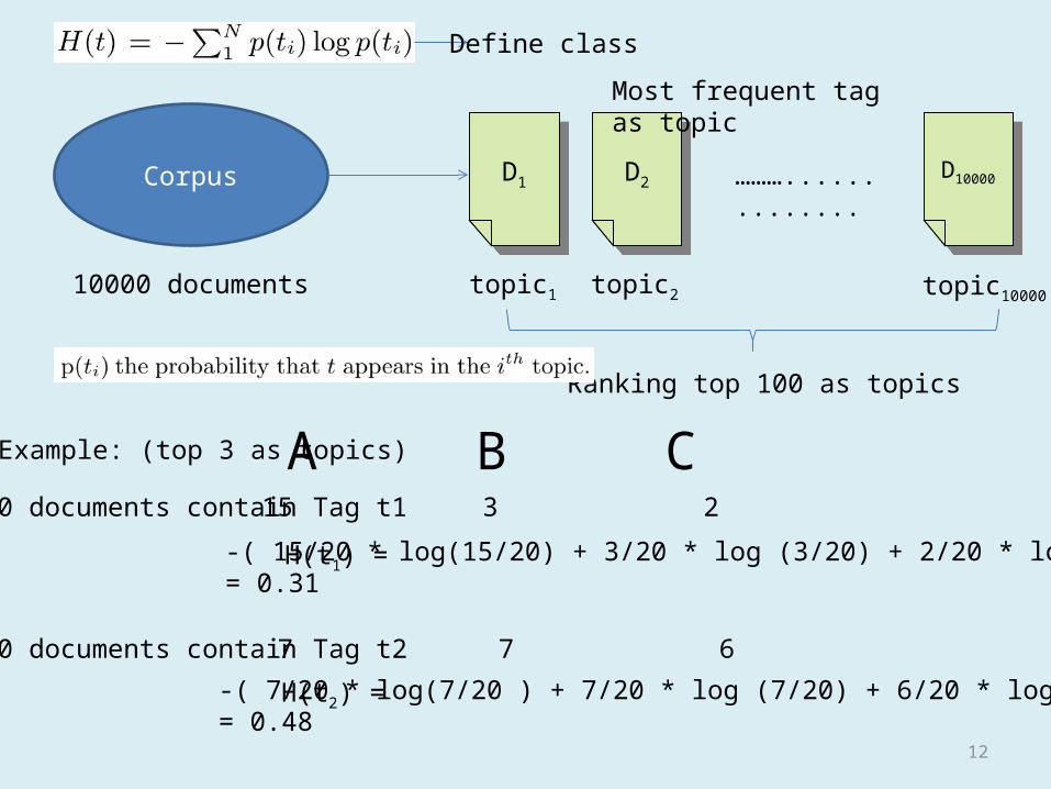
12
Define class
Corpus
10000 documents
D1D1 D2
D2 D10000D10000……….............
.
Most frequent tag as topic
topic1 topic2 topic10000
Ranking top 100 as topics
Example: (top 3 as topics) A B C20 documents contain Tag t1 15 3 2
-( 15/20 * log(15/20) + 3/20 * log (3/20) + 2/20 * log(2/20) )= 0.31
20 documents contain Tag t2 7 7 6
-( 7/20 * log(7/20 ) + 7/20 * log (7/20) + 6/20 * log(6/20) )= 0.48
H(t1) =
H(t2) =

13
Tag raw count C(t): The total number of appearance of tag t in a specific corpus.
C(money) = 12
C(basketball) = 8 + 9 + 9 = 26
Tag distinct count D(t): The total number of documents tagged by t.
D(NBA) = 3
D(foul) = 1
Money 12NBA 10
Basketball 8Player 5
PG 3
NBA 12Basketball 9
Injury 7Shoes 3Judge 3
Sports 10NBA 9
Basketball 9Foul 5
Injury 4
Economy 9Business 8
Salary 7Company 6Employee 2
Low-Paid 9Hospital 8
Nurse 7Doctor 7
Medicine 6
D1 D2 D3 D4 D5
14
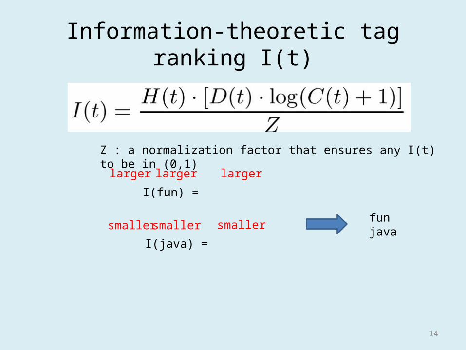
Information-theoretic tag ranking I(t)
Z : a normalization factor that ensures any I(t) to be in (0,1)
I(fun) =
I(java) =
larger larger larger
smaller smaller smallerfunjava

15
Global tag ranking
• Information-theoretic tag ranking I(t)– I(t) =
• Learning-to-rank based tag ranking Lr(t)– Lr(t) = H(t) + D(t)+ C(t)
w1 w2 w3

16
Learning-to-rank based tag ranking
traingingdata? Time-consuming
automatically generate

17
Learning-to-rank based tag ranking
Co(programming,java) = 200D(programming| − java) = 239 D(java| − programming) = 39
(programming,java) = = 6.12 > 2
Θ = 2 programming >r java

18
Learning-to-rank based tag ranking
1. Java2. Programming3. j2ee
Tags (T)
Θ = 2
< 0.3 10 50 >< 0.8 50 120 >< 0.2 7 10>
Feature vector
H ( t ) D ( t ) C ( t )
(Java, programming) =
(programming, j2ee) =
(x1,y1) = ({-0.5, -40, -70}, -1)(x2,y2) = ({0.6, 43, 110}, 1)
-1
+1

19
Learning-to-rank based tag ranking3498 distinct tags ---> 532 training examples
N = 3(Java, programming)(java, j2ee)(programming, j2ee)
(x1,y1) = ({-0.5, -40, -70}, -1)(x2,y2) = ({0.1, 3, 40}, 0)(x3,y3) = ({0.6, 43, 110}, 1)
L(T) = ─ (log g( y1 z1 ) + log g( y3 z3 )) + (
Z1 = w1 * (-0.5) + w2 * (-40) + w3 * (-70) Z3 = w1 * (0.6) + w2 * (43) + w3 * (110)
maximum L(T)
-1 1
g(z)
0 1
z = -oo z = oo
= 1
= 0.4
-40.15 57.08g(57.08) = 0.6g(-40.15) = 0.2
40.15 57.08g(57.08) = 0.6g(40.15) = 0.4

20
Learning-to-rank based tag ranking
w1
w2
w3
<H ( t ), D( t ), C( t )>Lr(tag)= X
= w1 * H(tag) + w2 * D(tag) + w3 * C(tag)

21
Global tag ranking

22
Constructing tag hierarchy
• Goal– select appropriate tags to be included in the tree– choose the optimal position for those tags
• Steps– Tree initialization– Iterative tag insertion– Optimal position selection
23
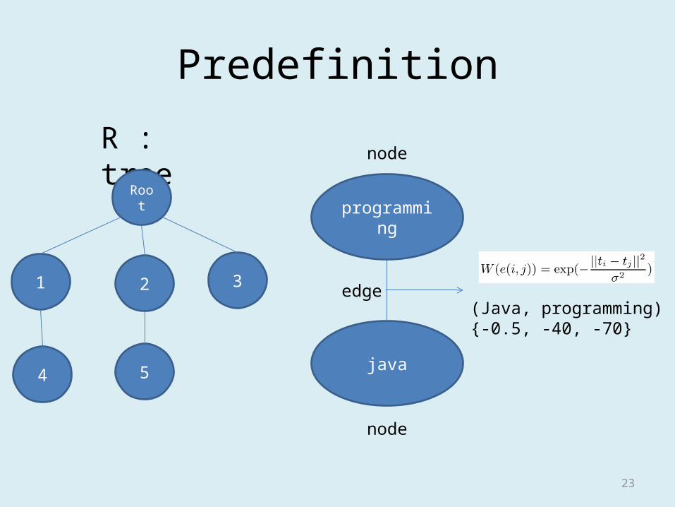
Predefinition
R : tree
1
Root
2 3
4 5
programming
java
node
node
edge(Java, programming){-0.5, -40, -70}

24
Predefinition
1
Root
2 3
4 5
0.3
0.1 0.3
0.40.2
d(ti,tj) : distance between two nodes
P(ti, tj) that connects them, through their lowest common ancestor LCA(ti, tj)
d(t1,t2) LCA(t1,t2) = ROOT
P(t1, t2) ROOT -> 1ROOT -> 2
d(t1,t2) = 0.3 + 0.4 = 0.7
d(t3,t5) LCA(t3,t5) = ROOT
P(t3, t5) ROOT -> 3ROOT -> 2, 2 -> 5
d(t3,t5) = 0.3 + 0.4 + 0.2 = 0.9

25
Predefinition
1
Root
2 3
4 5
0.3
0.1 0.3
0.40.2
Cost(R) = d(t1,t2) + d(t1,t3) + d(t1,t4) + d(t1,t5) +d(t2,t3) + d(t2,t4) + d(t2,t5) + d(t3,t4) +d(t3,t5) + d(t4,t5) = (0.3+0.4) + (0.3+0.2) + 0.1 + (0.3+0.4+0.3) +(0.4+0.2) + (0.3+0.1+0.4) + 0.3 + (0.3+0.1+0.2) +(0.4+0.3+0.2) + (0.3+0.1+0.4+0.3) = 6.6

26
Tree Initialization
ProgrammingNews
EducationEconomy
Sports.........
Ranked list
Top 1 to be root node?
programming
news
education
sports
.
.
. ...
.
.
.

27
Tree Initialization
27
ProgrammingNews
EducationEconomy
Sports.........
Ranked list
programming news educationsports
.
.
.
.
.
.
.
.
.
ROOT
.
.
.

28
Tree Initialization
Child(ROOT) = {reference, tools, web, design, blog, free}
ROOT ---- reference = Max{W(reference,tools), W(reference,web), W(reference,design), W(reference,blog),W(reference,free)}

29
Optimal position selection
1
Root
2 3
4 5
0.3
0.1 0.3
0.40.2
t1
t2
t3
t4
t5
Ranked list
t6
High costif the tree has depth L(R), then tnew can only be inserted at level L(R) or L(R)+1

30
Optimal position selection
1
Root
2 3
4 5
0.3
0.1 0.3
0.40.2
Cost(R) = d(t1,t2) + d(t1,t3) + d(t1,t4) + d(t1,t5) +d(t2,t3) + d(t2,t4) + d(t2,t5) + d(t3,t4) +d(t3,t5) + d(t4,t5) = (0.3+0.4) + (0.3+0.2) + 0.1 + (0.3+0.4+0.3) +(0.4+0.2) + (0.3+0.1+0.4) + 0.3 + (0.3+0.1+0.2) +(0.4+0.3+0.2) + (0.3+0.1+0.4+0.3) = 6.6
6
Cost(R’) = 6.6 + d(t1,t6) + d(t2,t6) + d(t3,t6) + d(t4,t6) + d(t5,t6) = 6.6+0.3+(0.4+0.6)+(0.2+0.6)+0.2+(0.7+0.6) = 10.2
0.2
0.2
6
6
0.2
0.2Cost(R’) = 6.6 + d(t1,t6) + d(t2,t6) + d(t3,t6) + d(t4,t6) + d(t5,t6) = 6.6+0.2+(0.4+0.5)+(0.2+0.5)+(0.1+0.2)+(0.7+0.6) +(0.7+0.5) = 11.2Cost(R’) = 6.6 + d(t1,t6) + d(t2,t6) + d(t3,t6) + d(t4,t6) + d(t5,t6) = 6.6+(0.3+0.9)+0.5+(0.2+0.9)+(0.4+0.9)+0.2= 10.96Cost(R’) = 6.6 + d(t1,t6) + d(t2,t6) + d(t3,t6) + d(t4,t6) + d(t5,t6) = 6.6+(0.3+0.6)+0.2+(0.2+0.6)+(0.4+0.6)+(0.3+0.2) = 10.0

31
Optimal position selection
1
Root
2
3
4
Cost(R) = d(t1,t2) + d(t1,t3) + d(t1,t4) +d(t2,t3) + d(t2,t4) + d(t3,t4)
Cost(R’) = d(t1,t2) + d(t1,t3) + d(t1,t4) +d(t2,t3) + d(t2,t4) + d(t3,t4) + d(t1,t4) + d(t2,t4) + d(t3,t4)
Consider both cost and the depth of tree
level
node counts
Root
1 2 3 4
5/log 5 = 7.14 2/log 5 = 2.85
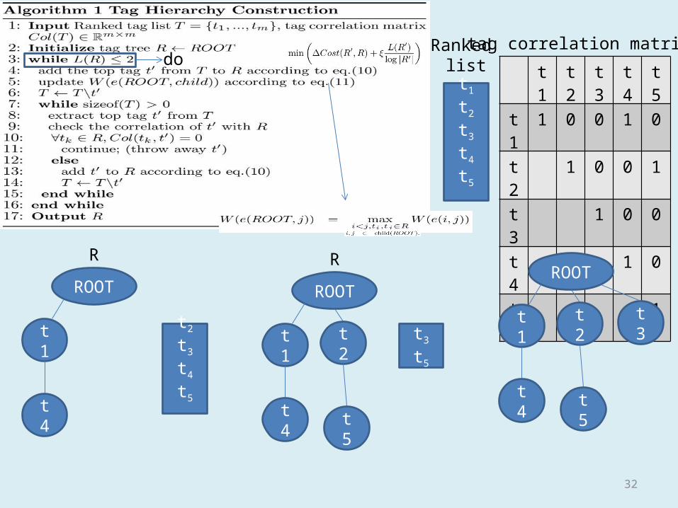
32
t1
t2
t3
t4
t5
Ranked list t1 t2 t3 t4 t5
t1 1 0 0 1 0
t2 1 0 0 1
t3 1 0 0
t4 1 0
t5 1
tag correlation matrix
ROOT
R
do
t1t2
t3
t4
t5
t4
ROOT
R
t1t3
t5
t4
t2
t5
ROOT
t1
t4
t2
t5
t3

33
Applications to tag recommendation
docdocdocdoc
Similarcontent
tags Tag recommendation
cost
docdoc 1
root
2 3
4 5
0.3
0.1 0.3
0.4 0.2Tag recommendation

34
Tag recommendation
docdoc
User-entered tags
1
root
2 3
4 5
0.3
0.1 0.3
0.4 0.2
Candidate tag list
recommendation tags
1. One user-entered tag2. Many user-entered tags3. No user-entered tag

35
docdoc
programming
technology webdesign
Candidate ={Software, development, computer, technology, tech, webdesign, java, .net}
Candidate ={Software, development, programming, apps, culture, flash, internet, freeware}

36
docdoc
Top k most frequent words from d appear in tag listpseudo tags

37
Tag recommendation

38
Tag recommendation
docdoc
technology webdesign
Candidate ={Software, development, programming, apps, culture, flash, internet, freeware}
Score(d, software | {technology, webdesign})= α (W(technology, software) + W(webdesign, software) ) + (1-α) N(software,d)
the number of times tag ti appears in document d
39
Experiment
• Data set– Delicious– 43113 unique tags and 36157 distinct URLs
• Efficiency of the tag hierarchy• Tag recommendation performance

40
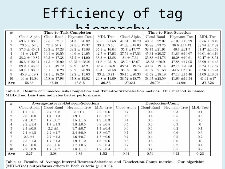
Efficiency of tag hierarchy
• Three time-related metric– Time-to-first-selection
• The time between the times-tamp from showing the page, and the timestamp of the first user tag selection
– Time-to-task-completion• the time required to select all tags for the task
– Average-interval-between-selections• the average time interval between adjacent selections of tags
• Additional metric– Deselection-count
• the number of times a user deselects a previously chosen tag and selects a more relevant one.

41
Efficiency of tag hierarchy
• 49 users• Tag 10 random web doc from delicious• 15 tag were presented with each web doc– User were asked for select 3 tags

42

43
Heymann tree
• A tag can be added as – A child node of the most similar tag node– A root node
44
Efficiency of tag hierarchy

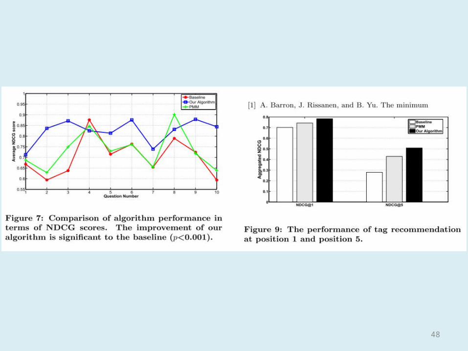
Tag recommendation performance
• Baseline: CF algorithm– Content-based– Document-word matrix– Cosine similarity– Top 5 similar web pages, recommend top 5 popular tags
• Our algorithm– Content-free
• PMM– Combined spectral clustering and mixture models
45

Tag recommendation performance
• Randomly sampled 10 pages• 49 users measure the relevance of recommended
tags(each page contains 5 tags)– Perfect(score 5),Excellent(score 4),Good(score 3),Fair
(score 2),Poor(score 1)• NDCG: normalized discounted cumulative gain– Rank– score
46

47
D1 D2 D3 D4 D5 D6
3, 2, 3, 0, 1, 2CG = 3 + 2 + 3 + 0 + 1 + 2 = 11
i reli log2(1+i) 2rel - 1
1 3 1 7
2 2 1.58 3
3 3 2 7
4 0 2.32 0
5 1 2.58 1
6 2 2.81 3
DCG = 7 + 1.9 + 3.5 + 0 + 0.39 + 1.07 = 13.86
IDCG: rel {3,3,2,2,1,0} = 7 + 4.43 + 1.5 + 1.29 + 0.39 = 14.61
NDCG = DCG / IDCG = 0.95
Each page has 5 recommended tags49 users to judgeAverage NDCG score
48
49
Conclusion
• We proposed a novel visualization of tag hierarchy which addresses two shortcomings of traditional tag clouds: – unable to capture the similarities between tags– unable to organize tags into levels of abstractness
• Our visualization method can reduce the tagging time• Our tag recommendation algorithm outperformed a
content-based recommendation method in NDCG scores