1 Gradient-Based Optimization - Stanford Universityadl.stanford.edu/aa222/Lecture_Notes_files/AA222-Lecture3.pdf · 1 Gradient-Based Optimization ... As in the single-variable case

1 Gradient-Based Optimization

1.1 General Algorithm for Smooth Functions

All algorithms for unconstrained gradient-based optimization can be described as follows. We

start with iteration number k = 0 and a starting point, xk.

1. Test for convergence. If the conditions for convergence are satisfied, then we can stop and

xk is the solution.

2. Compute a search direction. Compute the vector pk that defines the direction in n-space

along which we will search.

3. Compute the step length. Find a positive scalar, αk such that f(xk + αkpk) < f(xk).

4. Update the design variables. Set xk+1 = xk + αkpk, k = k + 1 and go back to 1.

xk+1 = xk + αkpk︸︷︷︸∆xk

(1)

There are two subproblems in this type of algorithm for each major iteration: computing the

search direction pk and finding the step size (controlled by αk). The difference between the

various types of gradient-based algorithms is the method that is used for computing the search

direction.

AA222: Introduction to MDO 1

1.2 Optimality Conditions

Consider a function f(x) where x is the n-vector x = [x1, x2, . . . , xn]T .

The gradient vector of this function is given by the partial derivatives with respect to each of

the independent variables,

∇f(x) ≡ g(x) ≡

∂f

∂x1∂f

∂x2...∂f

∂xn

(2)

In the multivariate case, the gradient vector is perpendicular to the the hyperplane tangent to

the contour surfaces of constant f .


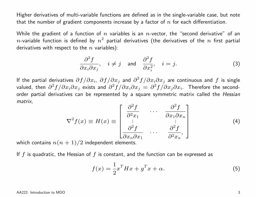
Higher derivatives of multi-variable functions are defined as in the single-variable case, but note

that the number of gradient components increase by a factor of n for each differentiation.

While the gradient of a function of n variables is an n-vector, the “second derivative” of an

n-variable function is defined by n2 partial derivatives (the derivatives of the n first partial

derivatives with respect to the n variables):

∂2f

∂xi∂xj, i 6= j and

∂2f

∂x2i

, i = j. (3)

If the partial derivatives ∂f/∂xi, ∂f/∂xj and ∂2f/∂xi∂xj are continuous and f is single

valued, then ∂2f/∂xi∂xj exists and ∂2f/∂xi∂xj = ∂2f/∂xj∂xi. Therefore the second-

order partial derivatives can be represented by a square symmetric matrix called the Hessian

matrix,

∇2f(x) ≡ H(x) ≡

∂2f

∂2x1

· · ·∂2f

∂x1∂xn... ...

∂2f

∂xn∂x1

· · ·∂2f

∂2xn,

(4)

which contains n(n+ 1)/2 independent elements.

If f is quadratic, the Hessian of f is constant, and the function can be expressed as

f(x) =1

2xTHx+ g

Tx+ α. (5)


As in the single-variable case the optimality conditions can be derived from the Taylor-series

expansion of f about x∗:

f(x∗

+ εp) = f(x∗) + εp

Tg(x

∗) +

1

2ε

2pTH(x

∗+ εθp)p, (6)

where 0 ≤ θ ≤ 1, ε is a scalar, and p is an n-vector.

For x∗ to be a local minimum, then for any vector p there must be a finite ε such that

f(x∗ + εp) ≥ f(x∗), i.e. there is a neighborhood in which this condition holds. If this

condition is satisfied, then f(x∗ + εp) − f(x∗) ≥ 0 and the first and second order terms in

the Taylor-series expansion must be greater than or equal to zero.

As in the single variable case, and for the same reason, we start by considering the first order

terms. Since p is an arbitrary vector and ε can be positive or negative, every component of the

gradient vector g(x∗) must be zero.

Now we have to consider the second order term, ε2pTH(x∗ + εθp)p. For this term to be

non-negative, H(x∗ + εθp) has to be positive semi-definite, and by continuity, the Hessian at

the optimum, H(x∗) must also be positive semi-definite.


Necessary conditions (for a local minimum):

‖g(x∗)‖ = 0 and H(x∗) is positive semi-definite. (7)

Sufficient conditions (for a strong local minimum):

‖g(x∗)‖ = 0 and H(x∗) is positive definite. (8)

Some definitions from linear algebra that might be helpful:

• The matrix H ∈ Rn×n is positive definite if pTHp > 0 for all nonzero vectors p ∈ Rn

(If H = HT then all the eigenvalues of H are strictly positive)

• The matrix H ∈ Rn×n is positive semi-definite if pTHp ≥ 0 for all vectors p ∈ Rn

(If H = HT then the eigenvalues of H are positive or zero)

• The matrix H ∈ Rn×n is indefinite if there exists p, q ∈ Rn such that pTHp > 0 and

qTHq < 0.

(If H = HT then H has eigenvalues of mixed sign.)

• The matrix H ∈ Rn×n is negative definite if pTHp < 0 for all nonzero vectors p ∈ Rn

(If H = HT then all the eigenvalues of H are strictly negative)


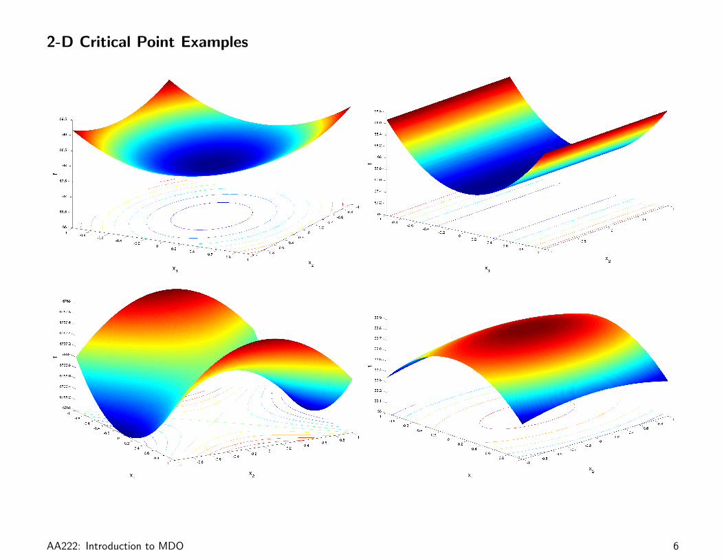
2-D Critical Point Examples


Example 1.1: Critical Points of a Function

Consider the function:

f(x) = 1.5x21 + x

22 − 2x1x2 + 2x

31 + 0.5x

41

Find all stationary points of f and classify them.

Solve ∇f(x) = 0, get three solutions:

(0, 0) local minimum

1/2(−3−√

7,−3−√

7) global minimum

1/2(−3 +√

7,−3 +√

7) saddle point

To establish the type of point, we have to determine if the Hessian is positive definite and

compare the values of the function at the points.


Figure 1: Critical points of f(x) = 1.5x21 + x2

2 − 2x1x2 + 2x31 + 0.5x4

1


1.3 Steepest Descent Method

The steepest descent method uses the gradient vector at each point as the search direction for

each iteration. As mentioned previously, the gradient vector is orthogonal to the plane tangent

to the isosurfaces of the function.

The gradient vector at a point, g(xk), is also the direction of maximum rate of change (maximum

increase) of the function at that point. This rate of change is given by the norm, ‖g(xk)‖.

Steepest descent algorithm:

1. Select starting point x0, and convergence parameters εg, εa and εr.

2. Compute g(xk) ≡ ∇f(xk). If ‖g(xk)‖ ≤ εg then stop. Otherwise, compute the

normalized search direction to pk = −g(xk)/‖g(xk)‖.

3. Perform line search to find step length αk in the direction of pk.

4. Update the current point, xk+1 = xk + αpk.

5. Evaluate f(xk+1). If the condition |f(xk+1) − f(xk)| ≤ εa + εr|f(xk)| is satisfied for

two successive iterations then stop. Otherwise, set k = k + 1, xk+1 = xk + 1 and return

to step 2.

Here, |f(xk+1)− f(xk)| ≤ εa + εr|F (xk)| is a check for the successive reductions of f . εais the absolute tolerance on the change in function value (usually small ≈ 10−6) and εr is the

relative tolerance (usually set to 0.01).


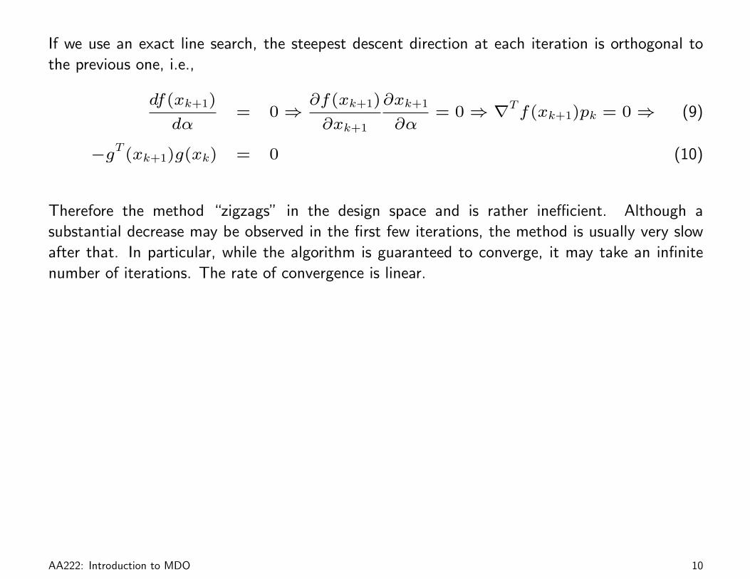
If we use an exact line search, the steepest descent direction at each iteration is orthogonal to

the previous one, i.e.,

df(xk+1)

dα= 0⇒

∂f(xk+1)

∂xk+1

∂xk+1

∂α= 0⇒ ∇T

f(xk+1)pk = 0⇒ (9)

−gT (xk+1)g(xk) = 0 (10)

Therefore the method “zigzags” in the design space and is rather inefficient. Although a

substantial decrease may be observed in the first few iterations, the method is usually very slow

after that. In particular, while the algorithm is guaranteed to converge, it may take an infinite

number of iterations. The rate of convergence is linear.


For steepest descent and other gradient methods that do not produce well-scaled search directions,

we need to use other information to guess a step length.

One strategy is to assume that the first-order change in xk will be the same as the one obtained

in the previous step. i.e, that αgTk pk = αk−1gTk−1pk−1 and therefore:

α = αk−1

gTk−1pk−1

gTk pk. (11)


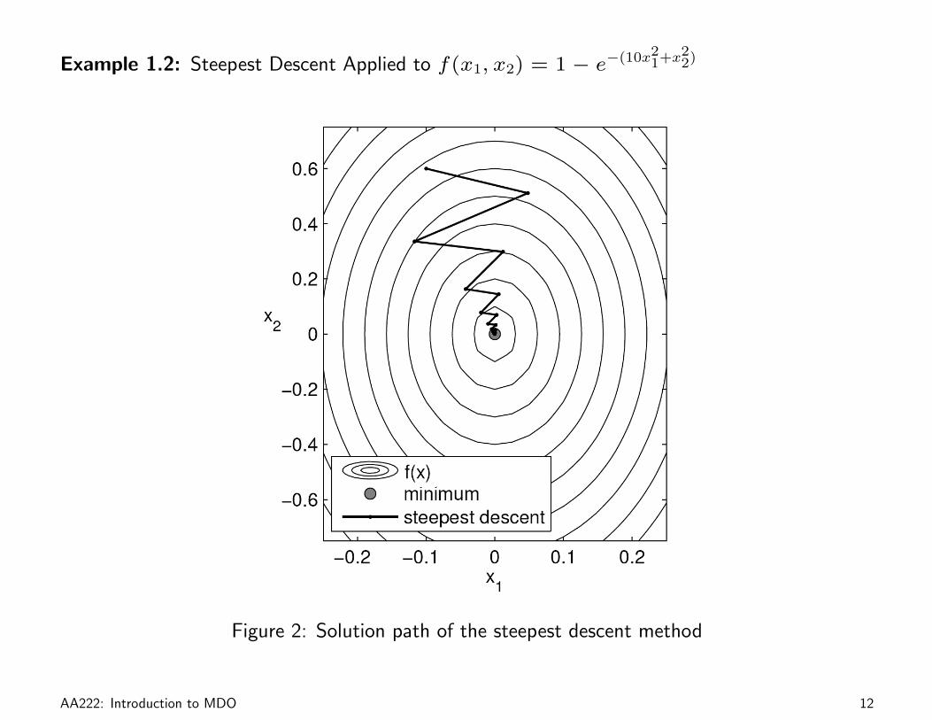
Example 1.2: Steepest Descent Applied to f(x1, x2) = 1− e−(10x21+x2

2)

Figure 2: Solution path of the steepest descent method


1.4 Conjugate Gradient Method

A small modification to the steepest descent method takes into account the history of the

gradients to move more directly towards the optimum.

Suppose we want to minimize a convex quadratic function

φ(x) =1

2xTAx− bTx (12)

where A is an n × n matrix that is symmetric and positive definite. Differentiating this with

respect to x we obtain,

∇φ(x) = Ax− b ≡ r(x). (13)

Minimizing the quadratic is thus equivalent to solving the linear system,

Ax = b. (14)

The conjugate gradient method is an iterative method for solving linear systems of equations

such as this one.

A set of nonzero vectors {p0, p1, . . . , pn−1} is conjugate with respect to A if

pTi Apj = 0, for all i 6= j. (15)


Suppose that we start from a point x0 and a set of directions {p0, p1, . . . , pn−1} to generate

a sequence {xk} where

xk+1 = xk + αkpk (16)

where αk is the minimizer of φ along xk + αpk, given by

αk = −rTk pk

pTkApk(17)

We will see that for any x0 the sequence {xk} generated by the conjugate direction algorithm

converges to the solution of the linear system in at most n steps.

Since conjugate directions are linearly independent, they span n-space. Therefore,

x∗ − x0 = σ0p0 + · · ·+ σn−1pn−1 (18)

Premultiplying by pTkA and using the conjugacy property we obtain

σk =pTkA(x∗ − x0)

pTkApk(19)


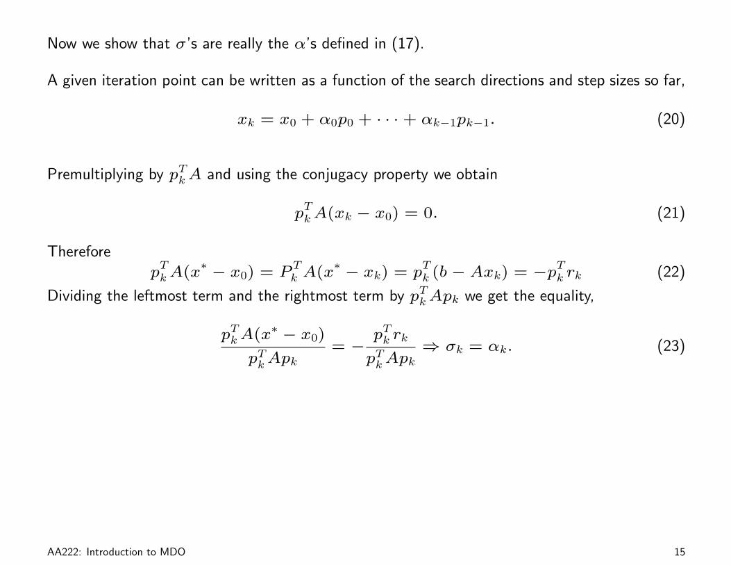
Now we show that σ’s are really the α’s defined in (17).

A given iteration point can be written as a function of the search directions and step sizes so far,

xk = x0 + α0p0 + · · ·+ αk−1pk−1. (20)

Premultiplying by pTkA and using the conjugacy property we obtain

pTkA(xk − x0) = 0. (21)

Therefore

pTkA(x

∗ − x0) = PTk A(x

∗ − xk) = pTk (b− Axk) = −pTk rk (22)

Dividing the leftmost term and the rightmost term by pTkApk we get the equality,

pTkA(x∗ − x0)

pTkApk= −

pTk rk

pTkApk⇒ σk = αk. (23)


There is a simple interpretation of the conjugate directions. If A is diagonal, the isosurfaces

are ellipsoids with axes aligned with coordinate directions. We could then find minimum by

performing univariate minimization along each coordinate direction in turn and this would result

in convergence to the minimum in n iterations.

When A a positive-definite matrix that is not diagonal, its contours are still elliptical, but they

are not aligned with the coordinate axes. Minimization along coordinate directions no longer

leads to solution in n iterations (or even a finite n).

If we transform the variables using

x = S−1x, (24)

where S =[p0 p1 · · · pn−1

], a matrix whose columns are the set of conjugate directions

with respect to A. The quadratic now becomes

φ(x) =1

2xT(STAS)x−

(STb)Tx (25)

By conjugacy,(STAS

)is diagonal so we can do a sequence of n line minimizations along

the coordinate directions of x. Each univariate minimization determines a component of x∗

correctly.


Nonlinear Conjugate Gradient Algorithm

(Also known as Fletcher–Reeves method)

1. Select starting point x0, and convergence parameters εg, εa and εr.

2. Compute g(xk) ≡ ∇f(xk). If ‖g(xk)‖ ≤ εg then stop.

3. If k = 0, then go to step 5.

4. Compute the new conjugate gradient direction pk = −gk + βkpk−1, where β =(‖gk‖‖gk−1‖

)2

=gTk gk

gTk−1

gk−1.

5. Perform line search to find step length αk in the direction of pk.

6. Update the current point, xk+1 = xk + αpk.

7. Evaluate f(xk+1). If the condition |f(xk+1) − f(xk)| ≤ εa + εr|f(xk)| is satisfied for

two successive iterations then stop. Otherwise, set k = k + 1 and return to step 3.


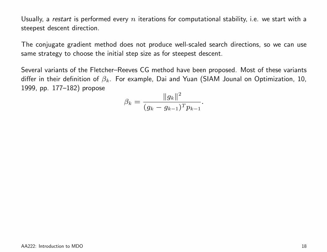
Usually, a restart is performed every n iterations for computational stability, i.e. we start with a

steepest descent direction.

The conjugate gradient method does not produce well-scaled search directions, so we can use

same strategy to choose the initial step size as for steepest descent.

Several variants of the Fletcher–Reeves CG method have been proposed. Most of these variants

differ in their definition of βk. For example, Dai and Yuan (SIAM Jounal on Optimization, 10,

1999, pp. 177–182) propose

βk =‖gk‖2

(gk − gk−1)Tpk−1

.


Example 1.3: Conjugate Gradient Applied to f(x1, x2) = 1− e−(10x21+x2

2)

Figure 3: Solution path of the nonlinear conjugate gradient method


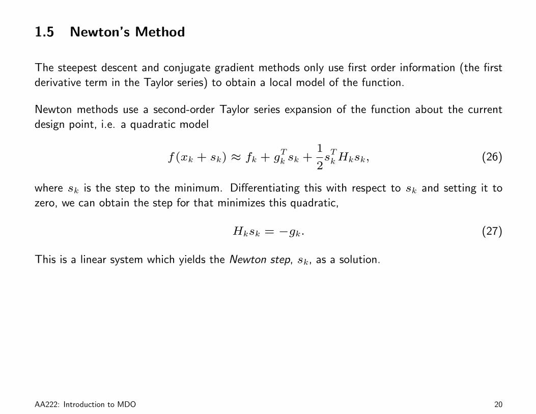
1.5 Newton’s Method

The steepest descent and conjugate gradient methods only use first order information (the first

derivative term in the Taylor series) to obtain a local model of the function.

Newton methods use a second-order Taylor series expansion of the function about the current

design point, i.e. a quadratic model

f(xk + sk) ≈ fk + gTk sk +

1

2sTkHksk, (26)

where sk is the step to the minimum. Differentiating this with respect to sk and setting it to

zero, we can obtain the step for that minimizes this quadratic,

Hksk = −gk. (27)

This is a linear system which yields the Newton step, sk, as a solution.


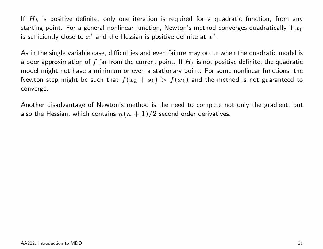
If Hk is positive definite, only one iteration is required for a quadratic function, from any

starting point. For a general nonlinear function, Newton’s method converges quadratically if x0

is sufficiently close to x∗ and the Hessian is positive definite at x∗.

As in the single variable case, difficulties and even failure may occur when the quadratic model is

a poor approximation of f far from the current point. If Hk is not positive definite, the quadratic

model might not have a minimum or even a stationary point. For some nonlinear functions, the

Newton step might be such that f(xk + sk) > f(xk) and the method is not guaranteed to

converge.

Another disadvantage of Newton’s method is the need to compute not only the gradient, but

also the Hessian, which contains n(n+ 1)/2 second order derivatives.


Modified Newton’s Method

A small modification to Newton’s method is to perform a line search along the Newton direction,

rather than accepting the step size that would minimize the quadratic model.

1. Select starting point x0, and convergence parameter εg.

2. Compute g(xk) ≡ ∇f(xk). If ‖g(xk)‖ ≤ εg then stop. Otherwise, continue.

3. Compute H(xk) ≡ ∇2f(xk) and the search direction, pk = −H−1gk.

4. Perform line search to find step length αk in the direction of pk (start with αk = 1).

5. Update the current point, xk+1 = xk + αkpk and return to step 2.

Although this modification increases the probability that f(xk+pk) < f(xk), it still vulnerable

to the problem of having an Hessian that is not positive definite and has all the other disadvantages

of the pure Newton’s method.

We could also introduce a modification to use a symmetric positive definite matrix instead of

the real Hessian to ensure descent:

Bk = Hk + γI,

where γ is chosen such that all the eigenvalues are greater than a tolerance δ > 0 (if δ is too

close to zero, Bk might be ill-conditioned, which can lead to round of errors in the solution of

the linear system).


When using Newton or quasi-Newton methods, the starting step length α is usually set to 1,

since Newton’s method already provides a good guess for the step size.

The step size reduction ratio (ρ in the backtracking line search) sometimes varies during the

optimization process and is such that 0 < ρ < 1. In practice ρ is not set to be too close to 0

or 1.


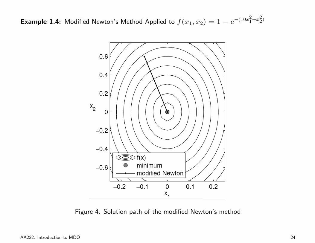
Example 1.4: Modified Newton’s Method Applied to f(x1, x2) = 1− e−(10x21+x2

2)

Figure 4: Solution path of the modified Newton’s method


1.6 Quasi-Newton Methods

This class of methods uses first order information only, but build second order information — an

approximate Hessian — based on the sequence of function values and gradients from previous

iterations. Most of these methods also force the Hessian to be symmetric and positive definite,

which can greatly improve their convergence properties.

When using quasi-Newton methods, we usually start with the Hessian initialized to the identity

matrix and then update it at each iteration. Since what we actually need is the inverse of the

Hessian, we will work with Vk ≈ H−1k . The update at each iteration is written as Vk and is

added to the current one,

Vk+1 = Vk + Vk. (28)

Let sk be the step taken from xk, and consider the Taylor-series expansion of the gradient

function about xk,

g(xk + sk) = gk +Hksk + · · · (29)

Truncating this series and setting the variation of the gradient to yk = g(xk + sk)− gk yields

Hksk = yk. (30)

Then, the new approximate inverse of the Hessian, Vk+1 must satisfy the quasi-Newton condition,

Vk+1yk = sk. (31)


1.6.1 Davidon–Fletcher–Powell (DFP) Method

One of the first quasi-Newton methods was devised by Davidon (1959) and modified by Fletcher

and Powell (1963).

Suppose we model the objective function as a quadratic at the current iterate xk:

φk(p) = fk + gTk p+

1

2pTBkp, (32)

where Bk is an n× n symmetric positive definite matrix that is updated every iteration.

The minimizer pk for this convex quadratic model can be written as,

pk = −B−1k gk. (33)

This solution is used to compute the search direction to obtain the new iterate

xk+1 = xk + αkpk (34)

where αk is obtained using a line search.

This is the same procedure as the Newton method, except that we use an approximate Hessian

Bk instead of the true Hessian.


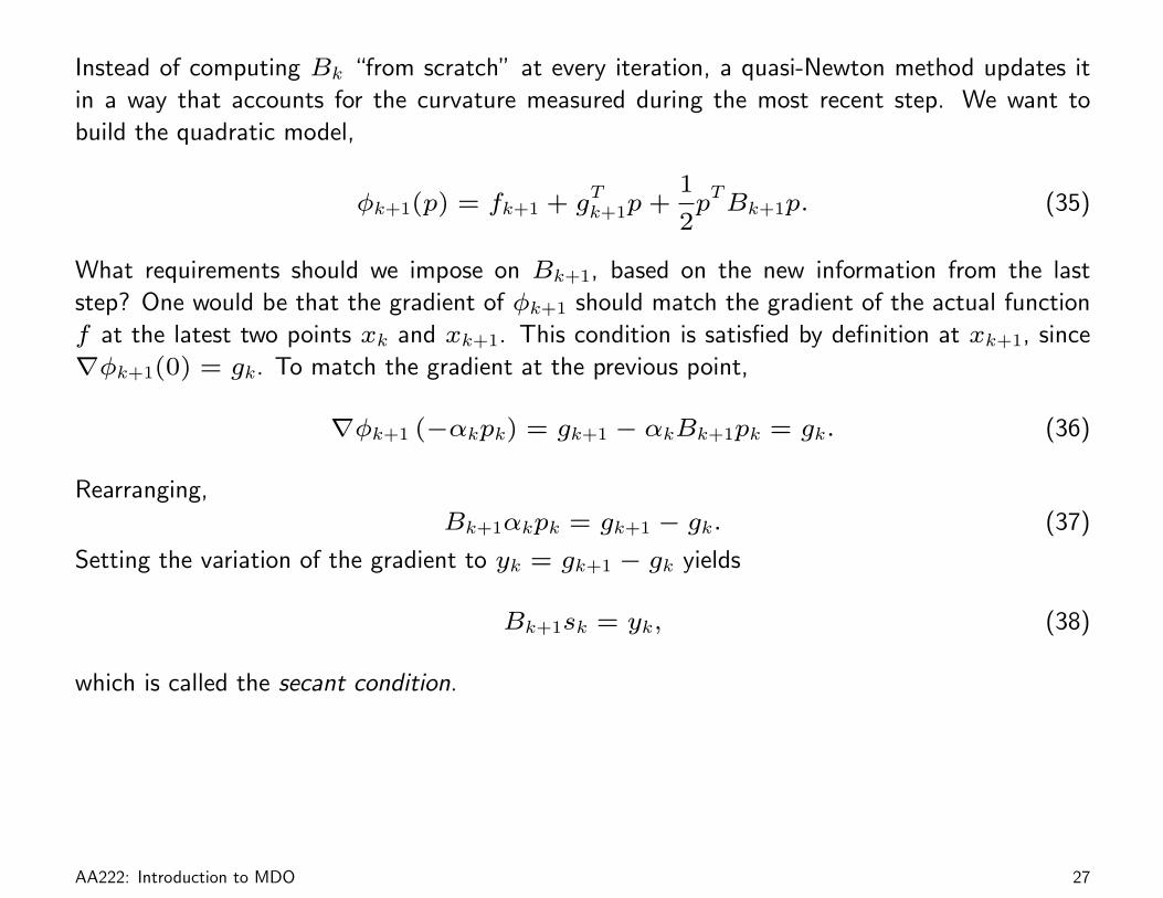
Instead of computing Bk “from scratch” at every iteration, a quasi-Newton method updates it

in a way that accounts for the curvature measured during the most recent step. We want to

build the quadratic model,

φk+1(p) = fk+1 + gTk+1p+

1

2pTBk+1p. (35)

What requirements should we impose on Bk+1, based on the new information from the last

step? One would be that the gradient of φk+1 should match the gradient of the actual function

f at the latest two points xk and xk+1. This condition is satisfied by definition at xk+1, since

∇φk+1(0) = gk. To match the gradient at the previous point,

∇φk+1 (−αkpk) = gk+1 − αkBk+1pk = gk. (36)

Rearranging,

Bk+1αkpk = gk+1 − gk. (37)

Setting the variation of the gradient to yk = gk+1 − gk yields

Bk+1sk = yk, (38)

which is called the secant condition.


We have n(n+ 1)/2 unknowns and only n equations, so this system has an infinite number of

solutions for Bk+1. To determine the solution uniquely, we impose a condition that among all

the matrices that satisfy the secant condition, selects the Bk+1 that is “closest” to the previous

Hessian approximation Bk, i.e. we solve,

minimize ‖B − Bk‖ (39)

with respect to B (40)

subject to B = BT , Bsk = yk. (41)

Using different matrix norms result in different quasi-Newton methods. One norm that makes

it easy to solve this problem and possesses good numerical properties is the weighted Frobenius

norm

‖A‖W = ‖W 1/2AW

1/2‖F , (42)

where the norm is defined as ‖C‖F =∑n

i=1

∑nj=1 c

2ij. The weights W are chosen to satisfy

certain favorable conditions.

For further details on the derivation of the quasi-Newton methods, see Dennis and More’s review

(SIAM Review, Vol. 19, No. 1, 1977).


Using this norm and weights, the unique solution of the norm minimization problem (39) is,

Bk+1 =

(I −

yksTk

yTk sk

)Bk

(I −

skyTk

yTk sk

)+yky

Tk

yTk sk, (43)

which is the DFP updating formula originally proposed by Davidon.

Using the inverse of Bk is usually more useful, since the search direction can then be obtained

by matrix multiplication. Defining,

Vk = B−1k . (44)

The DFP update for the inverse of the Hessian approximation can be shown to be

Vk+1 = Vk −Vkyky

Tk Vk

yTk Vkyk+sks

Tk

yTk sk(45)


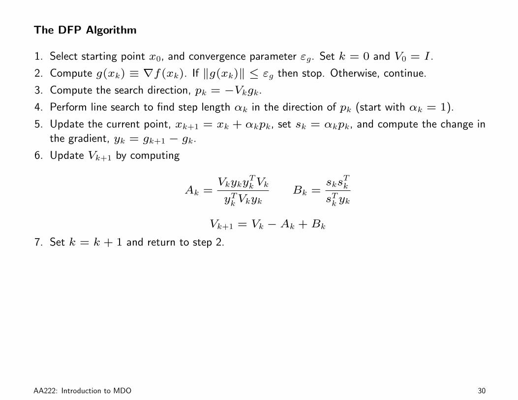
The DFP Algorithm

1. Select starting point x0, and convergence parameter εg. Set k = 0 and V0 = I.


3. Compute the search direction, pk = −Vkgk.

4. Perform line search to find step length αk in the direction of pk (start with αk = 1).

5. Update the current point, xk+1 = xk + αkpk, set sk = αkpk, and compute the change in

the gradient, yk = gk+1 − gk.

6. Update Vk+1 by computing

Ak =Vkyky

Tk Vk

yTk VkykBk =

sksTk

sTk yk

Vk+1 = Vk − Ak + Bk

7. Set k = k + 1 and return to step 2.


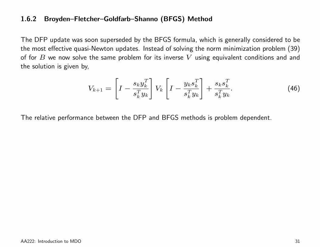
1.6.2 Broyden–Fletcher–Goldfarb–Shanno (BFGS) Method

The DFP update was soon superseded by the BFGS formula, which is generally considered to be

the most effective quasi-Newton updates. Instead of solving the norm minimization problem (39)

of for B we now solve the same problem for its inverse V using equivalent conditions and and

the solution is given by,

Vk+1 =

[I −

skyTk

sTk yk

]Vk

[I −

yksTk

sTk yk

]+sks

Tk

sTk yk. (46)

The relative performance between the DFP and BFGS methods is problem dependent.


Example 1.5: BFGS Applied to f(x1, x2) = 1− e−(10x21+x2

2)

Figure 5: Solution path of the BFGS method


1.6.3 Symmetric Rank-1 Update Method (SR1)

If we drop the requirement that the approximate Hessian (or its inverse) be positive definite, we

can derive a simple rank-1 update formula for Bk that maintains the symmetry of the matrix

and satisfies the secant equation. Such a formula is given by the symmetric rank-1 update (SR1)

method (we use the Hessian update here, and not the inverse Vk):

Bk+1 = Bk +(yk − Bksk)(yk − Bksk)

T

(yk − Bksk)Tsk.

With this formula, we must consider the cases when the denominator vanishes, and add the

necessary safe-guards:

1. if yk = Bksk then the only update that satisfies the secant equation is Bk+1 = Bk (i.e. do

not change the matrix).

2. if yk 6= Bksk and (yk − Bksk)Tsk = 0 then there is no symmetric rank-1 update that

satisfies the secant equation.

To avoid the second case, we update the matrix only if the following condition is met:

|yTk (sk − Bkyk)| ≥ r‖sk‖‖yk − Bksk‖,

where r ∈ (0, 1) is a small number (e.g. r = 10−8). Hence, if this condition is not met, we

use Bk+1 = Bk.


Why would we be interested in a Hessian approximation that is potentially indefinite? In practice,

the matrices produced by SR1 have been found to approximation the true Hessian matrix very

well (often better than BFGS). This may be useful in trust-region methods (see next section)

or constrained optimization problems; in the latter case the Hessian of the Lagrangian is often

indefinte, even at the minimizer.

To use the SR1 method in practice, it may be necessary to add a diagonal matrix γI to Bk

when calulating the serach direction, as was done in modified Newton’s method. In addition, a

simple back-tracking line search can be used, since the Wolfe conditions are not required as part

of the update (unlike BFGS).


Example 1.6: Minimization of the Rosenbrock Function

Minimize Rosenbrock’s function,

f(x) = 100(x2 − x2

1

)2

+ (1− x1)2,

starting from x0 = (−1.2, 1.0)T .


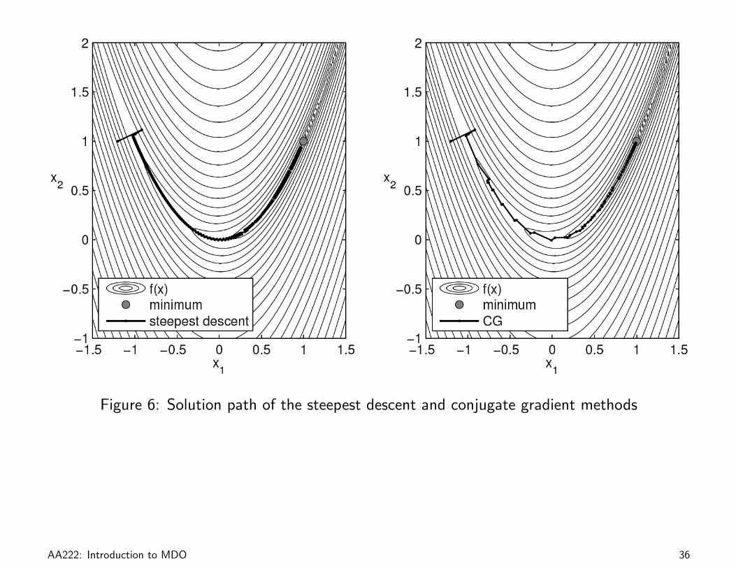
Figure 6: Solution path of the steepest descent and conjugate gradient methods


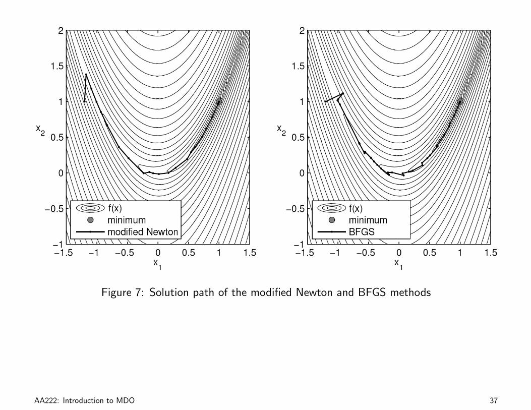
Figure 7: Solution path of the modified Newton and BFGS methods


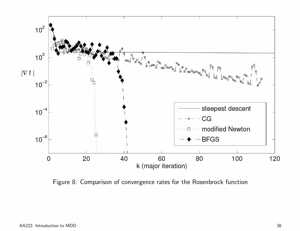
Figure 8: Comparison of convergence rates for the Rosenbrock function


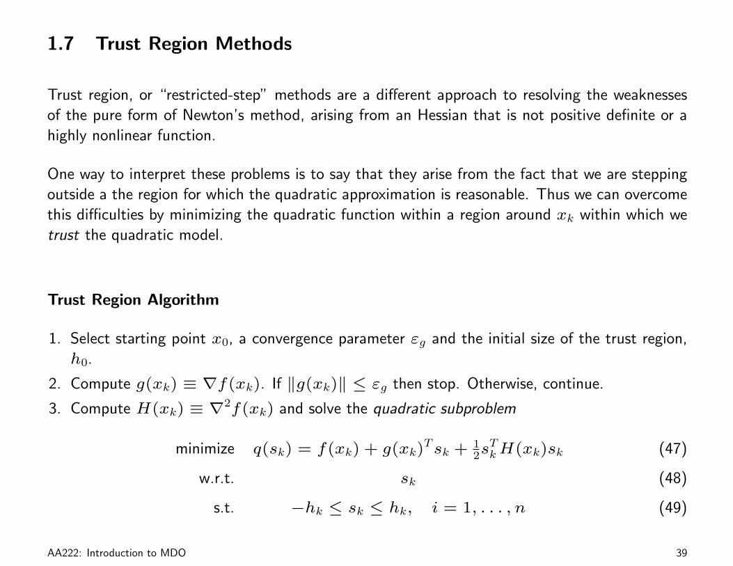
1.7 Trust Region Methods

Trust region, or “restricted-step” methods are a different approach to resolving the weaknesses

of the pure form of Newton’s method, arising from an Hessian that is not positive definite or a

highly nonlinear function.

One way to interpret these problems is to say that they arise from the fact that we are stepping

outside a the region for which the quadratic approximation is reasonable. Thus we can overcome

this difficulties by minimizing the quadratic function within a region around xk within which we

trust the quadratic model.

Trust Region Algorithm

1. Select starting point x0, a convergence parameter εg and the initial size of the trust region,

h0.


3. Compute H(xk) ≡ ∇2f(xk) and solve the quadratic subproblem

minimize q(sk) = f(xk) + g(xk)Tsk + 1

2sTkH(xk)sk (47)

w.r.t. sk (48)

s.t. −hk ≤ sk ≤ hk, i = 1, . . . , n (49)


4. Evaluate f(xk + sk) and compute the ratio that measures the accuracy of the quadratic

model,

rk =∆f

∆q=f(xk)− f(xk + sk)

f(xk)− q(sk).

5. Compute the size for the new trust region as follows:

hk+1 =‖sk‖

4if rk < 0.25, (50)

hk+1 = 2hk if rk > 0.75 and hk = ‖sk‖, (51)

hk+1 = hk otherwise. (52)

6. Determine the new point:

xk+1 = xk if rk ≤ 0 (53)

xk+1 = xk + sk otherwise. (54)

7. Set k = k + 1 and return to 2.

The initial value of h is usually 1. The same stopping criteria used in other gradient-based

methods are applicable.


References

[1] A. D. Belegundu and T. R. Chandrupatla. Optimization Concepts and Applications in

Engineering, chapter 3. Prentice Hall, 1999.

[2] J. Nocedal and S. J. Wright. Numerical Optimization. Springer, 2nd edition, 2006.

[3] C. Onwubiko. Introduction to Engineering Design Optimization, chapter 4. Prentice Hall,

2000.


Documents

1 Gradient-Based Optimization - Stanford Universityadl.stanford.edu/aa222/Lecture_Notes_files/AA222-Lecture3.pdf · 1 Gradient-Based Optimization ... As in the single-variable case