1 Geometric Primitives Chapter 1 - avida.cs.wright.edu

1-1Department of Computer Science and Engineering

1 Geometric Primitives

Chapter 1

Geometric Primitives



1.1 OverviewThe main goal of three-dimensional computer graphics is to generate two-dimensional images of a scene or of an object based on a description or a model.The internal representation of an object depends on several implications:

– The object may be a real object or it exists only as a computer representation

– The manufacturing of the object is bound closely to the visualization:

• Interactive CAD systems• Modeling and visualization as a tool during design and

manufacturing• More than just 2-D output possible!



1.1 OverviewImplications (continued)

– The precision of the internal computer representation depends on the application. For example, an exact description of the geometry and shape in CAD applications vs. an approximation sufficient for rendering of the object.

– For interactive applications, the object may be described by several internal representations. These representations may be generated in advance or on-the-fly.

• Level-of-detail (LOD) techniques



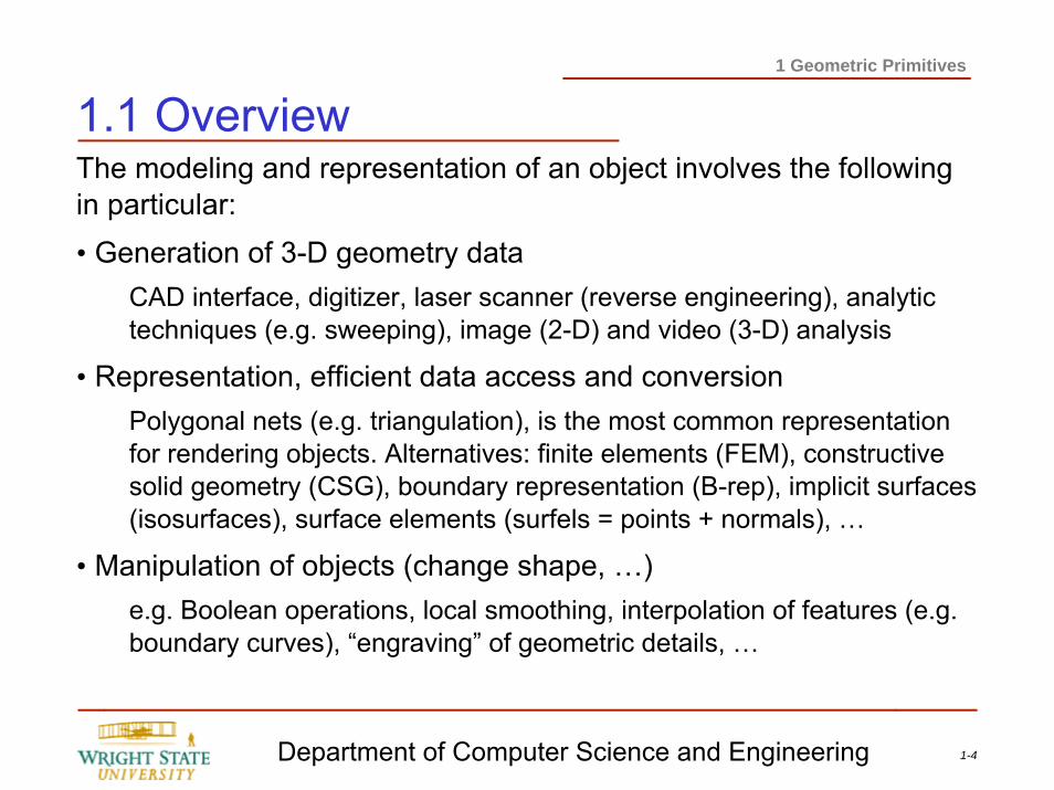
1.1 OverviewThe modeling and representation of an object involves the following in particular:• Generation of 3-D geometry data

CAD interface, digitizer, laser scanner (reverse engineering), analytic techniques (e.g. sweeping), image (2-D) and video (3-D) analysis

• Representation, efficient data access and conversionPolygonal nets (e.g. triangulation), is the most common representation for rendering objects. Alternatives: finite elements (FEM), constructive solid geometry (CSG), boundary representation (B-rep), implicit surfaces (isosurfaces), surface elements (surfels = points + normals), …

• Manipulation of objects (change shape, …)e.g. Boolean operations, local smoothing, interpolation of features (e.g. boundary curves), “engraving” of geometric details, …



1.1 OverviewThe topics of this chapter will be:

– Video display devices– Introduction to OpenGL– Geometric primitives– Rendering primitives with OpenGL– Rendering primitives on raster displays



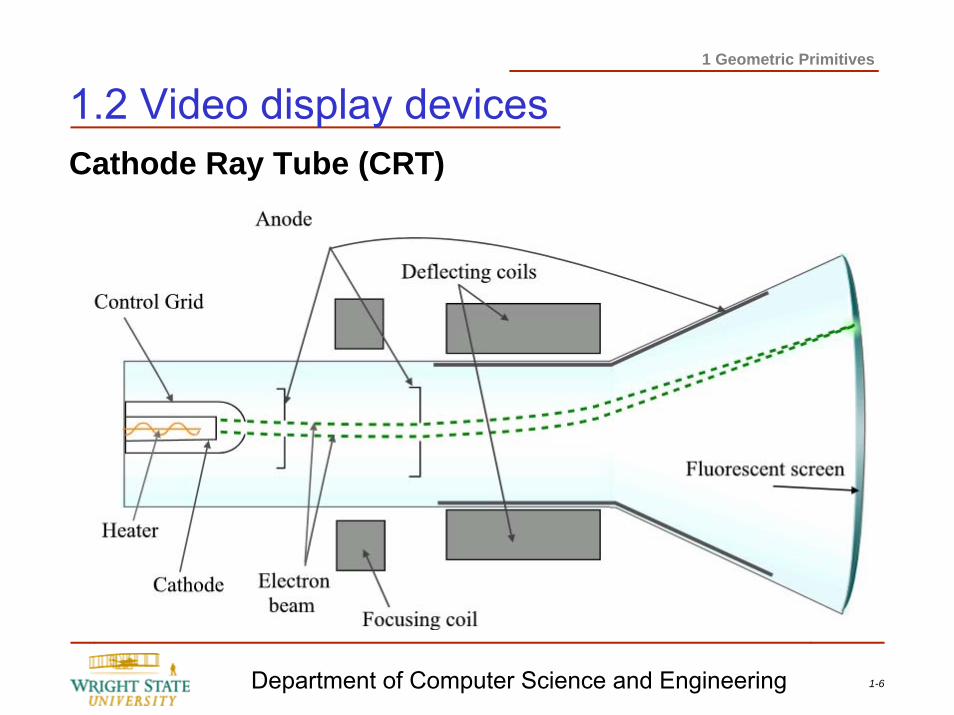
1.2 Video display devicesCathode Ray Tube (CRT)



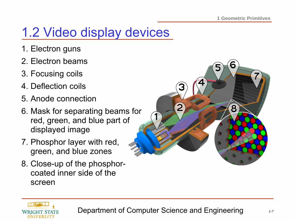
1.2 Video display devices1. Electron guns 2. Electron beams 3. Focusing coils 4. Deflection coils 5. Anode connection 6. Mask for separating beams for

red, green, and blue part of displayed image

7. Phosphor layer with red, green, and blue zones

8. Close-up of the phosphor-coated inner side of the screen



1.2 Video display devicesThin-Film-Transistor (TFT) displaysThe display consists of a raster of thin-film-transistors of different color (red, green, and blue) for every pixel. These do not emit light by themselves but change the polarization of incoming light. Hence, a TFT display deploys two polarization filters to let light from a back light (usually fluorescent) pass or block it.Most commonly used are twisted-nematic TFS, which are explained on the next two slide.



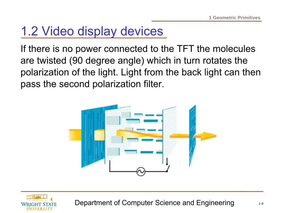
1.2 Video display devicesIf there is no power connected to the TFT the molecules are twisted (90 degree angle) which in turn rotates the polarization of the light. Light from the back light can then pass the second polarization filter.



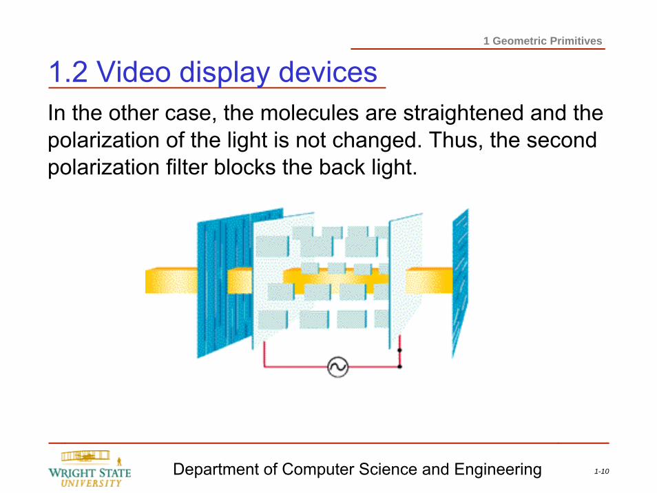
1.2 Video display devicesIn the other case, the molecules are straightened and the polarization of the light is not changed. Thus, the second polarization filter blocks the back light.



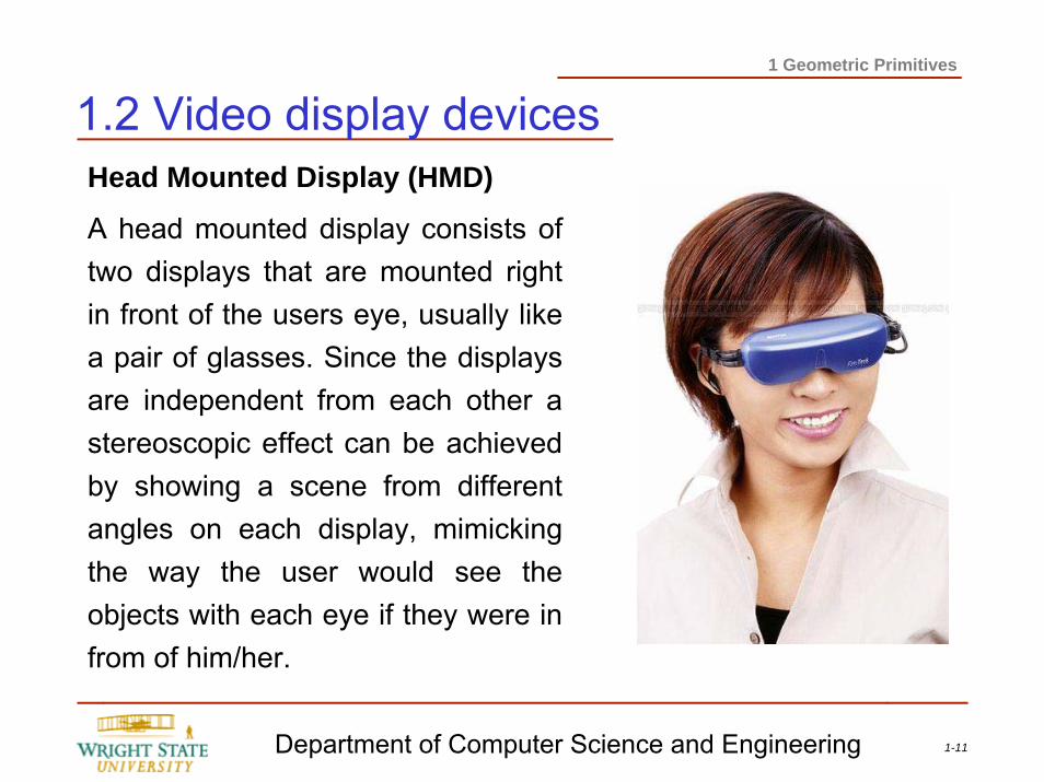
Head Mounted Display (HMD)

A head mounted display consists of two displays that are mounted right in front of the users eye, usually like a pair of glasses. Since the displays are independent from each other a stereoscopic effect can be achieved by showing a scene from different angles on each display, mimicking the way the user would see the objects with each eye if they were in from of him/her.

1.2 Video display devices



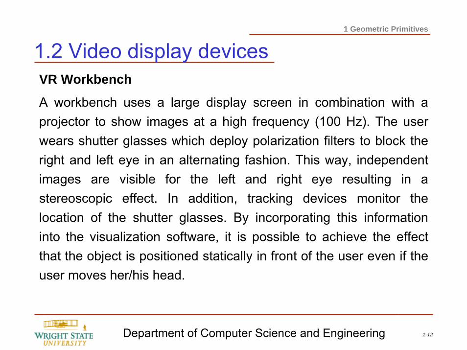
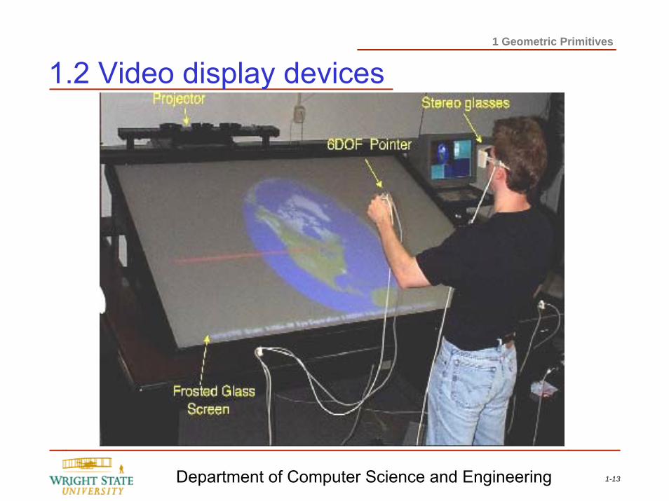
VR Workbench

A workbench uses a large display screen in combination with a projector to show images at a high frequency (100 Hz). The user wears shutter glasses which deploy polarization filters to block the right and left eye in an alternating fashion. This way, independent images are visible for the left and right eye resulting in a stereoscopic effect. In addition, tracking devices monitor the location of the shutter glasses. By incorporating this information into the visualization software, it is possible to achieve the effect that the object is positioned statically in front of the user even if the user moves her/his head.







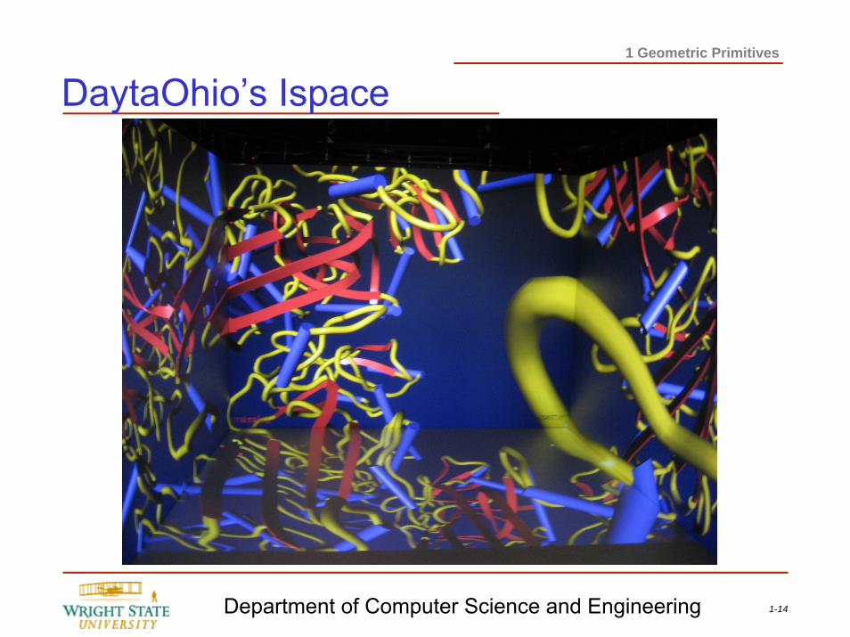
DaytaOhio’s Ispace



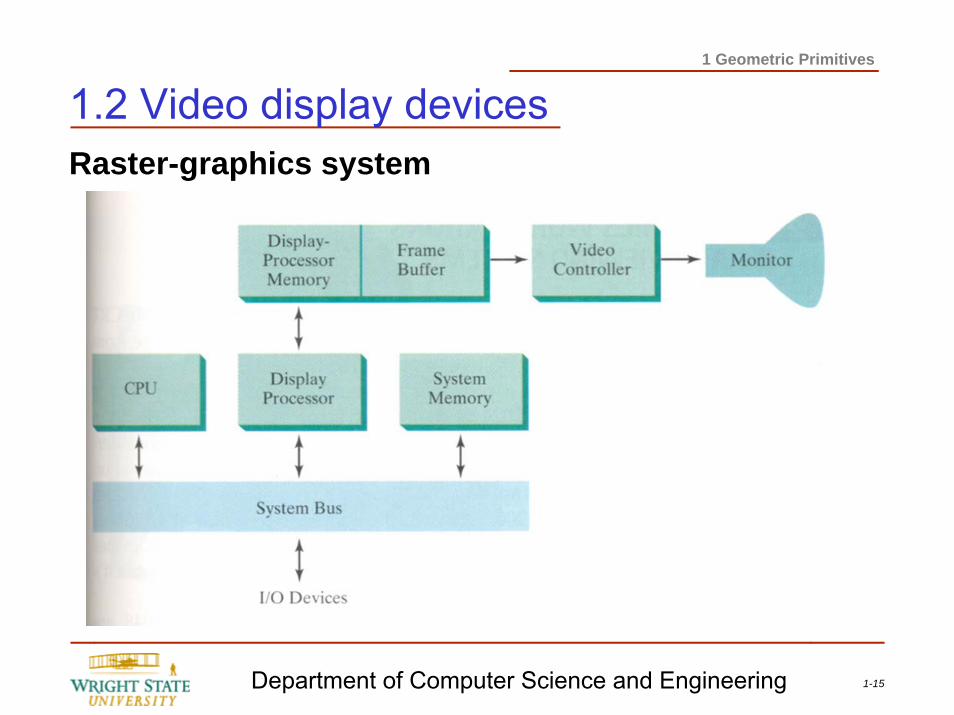
1.2 Video display devicesRaster-graphics system



1.3 Introduction to OpenGLBasicsEvery basic OpenGL function is prefixed with gl, followed by a capital letter. For example:

glBegin, glClear, glCopyPixels, …

Certain functions require that one (or more) of their arguments be assigned a symbolic constant. All such constants begin with the uppercase letters GL. In addition, component words within a constant name are capitalized:

GL_2D, GL_RGB, GL_POLYGON, …



1.3 Introduction to OpenGLThe OpenGL functions also expect specific data types. To indicate a specific data type, OpenGL uses special built-in data-type names, such as:

GLbyte, GLshort, GLint, GLfloat, GLdouble, GLboolean

Each data type name begins with the capital letters GLand the remainder of the name is a standard data-type designation, written in lower-case letters.These data types are usually mapped to the standard C equivalents. However, there is no guaranty. Hence, it is advisable to use the standard OpenGL date types.



1.3 Introduction to OpenGLRelated librariesIn addition to the OpenGL library, there are a number of associated libraries for handling special operations. The OpenGL Utility (GLU) library provides routines for setting up viewing and projection matrices, describing complex objects with line and polygon approximations, displaying quadrics and B-spline using linear approximations, processing the surface-rendering operations, and other complex tasks. Every OpenGL implementation includes the GLU library, and all GLU function names start with the prefix glu.



1.3 Introduction to OpenGLOpenGL is platform independent. However, special methods are necessary for opening a window on a specific system. Therefore, several window system libraries are available that support OpenGL functions for a variety of machines.The OpenGL Extension to the X Window System (GLX) provides a set of routines that are prefixed with the letters glX and used for X11/Unix systems. Apple systems can use the Apple GL (AGL) interface for window-management operations. Function names for this library are prefixed agl. For Microsoft Windows systems, the WGL routines provide a Windows-to-OpenGLinterface. These routines are prefixed with the letters wgl.



1.3 Introduction to OpenGLIn addition, the OpenGL Utility Toolkit (GLUT) provides a library of functions for interacting with any screen-windowing system. The GLUT library functions are prefixed with glut, and this library also contains methods for describing and rendering quadric curves and surfaces.Since GLUT is an interface to other device-specific window systems, we can use GLUT so that our programs will be device independent.You can find more about GLUT at the web site:http://www.opengl.org/documentation/specs/glut/spec3/spec3.html

A windows version of the GLUT library is available here:http://www.xmission.com/~nate/glut.html



1.3 Introduction to OpenGLHeader filesIn all of our graphics programs, we will need to include the header file for the OpenGL core library. For most applications we will also need GLU.

#include <GL/gl.h>

#include <GL/glu.h>

However, if we use GLUT to handle the window-managing operations, we do not need to include gl.h and glu.h because GLUT ensures that these will be included correctly. Thus we can replace the header files for OpenGL and GLU with

#include <GL/glut.h>



1.3 Introduction to OpenGLDisplay-Window Management using GLUTTo get started, we can consider a simplified, minimal number of operations for displaying a picture. Since we are using the OpenGL Utility Toolkit, our first step is to initialize GLUT. This initialization function could also process any command-line arguments:

glutInit (&argc, argv);

Next, we can state that a display window is to be created on the screen with a given caption for the title bar:

glCreateWindow (“Title bar”);



1.3 Introduction to OpenGLThen we need to specify what the display window is to contain. For this, we create a picture using OpenGL functions and pass the picture definition to the GLUT routine glutDisplayFunc, which assigns our picture to the display window:

glutDisplayFunc (display);

But the display window is not yet on the screen. We need one more GLUT function to complete the window-processing operations. After execution of the following statement, all display windows that we created, including their graphic content, are now activated.

glutMainLoop ();



1.3 Introduction to OpenGLIn addition, we can specify the window location and window size,respectively, using:

glutInitWindowPosition (50, 100);

glutInitWindowSize (400, 300);

Even after the window is displayed, these methods can be used toresize or reposition it.There are also a number of parameters that can be specified to what kind of display window is desired. These parameters are specified as symbolic GLUT constants. For example, the following command specifies that a single refresh buffer is to be used for the display window and that the RGB (red, green, blue) color mode is to be used for selecting color values:

glutInitDisplayMode (GLUT_SINGLE | GLUT_RGB);



1.3 Introduction to OpenGLAt this point, we did not draw anything yet. Hence, the display routine that we specified before needs to be implemented.First, we need to set a background color. Using RGB color values, we set the background color for the display window to be white with the OpenGL function

glClearColor (1.0, 1.0, 1.0, 0.0);

The first three parameters specify the color values for red, green, and blue, respectively, on a scale between 0.0and 1.0. The last parameter determines the alpha value, i.e. how transparent the background is going to be.



1.3 Introduction to OpenGLThis, however, does not actually clear the window. Therefore, we need to issue the following command:

glClear (GL_COLOR_BUFFER_BIT);

The argument GL_COLOR_BUFFER_BIT is an OpenGL symbolic constant specifying that it is the bit values in the color buffer (refresh buffer, frame buffer) that are to be set to the values indicated in the glClearColor function.There are other arguments that are often used (which are combined using a logical or). But for now, clearing the color buffer will suffice.



1.3 Introduction to OpenGLIn addition to setting the background color for the display window, we can choose a variety of color schemes for the objects we want to display in a scene. For our initial programming example, we will simply set object color to be red and defer further discussion of the various color options until later:

glColor3f (1.0, 0.0, 0.0);

The suffix 3f on the glColor function indicates that we are specifying the three RGB color components using floating-point (f) values. These values must be in the range from 0.0, to 1.0, and we have set red=1.0 and green = blue = 0.0.



1.3 Introduction to OpenGLFor our first, program we simply display a two-dimensional line segment. To do this, we need to tell OpenGL how we want to “project” our picture onto the display window, because generating a two-dimensional picture is treated by OpenGL as a special case of three-dimensional viewing:

glMatrixMode (GL_PROJECTION);gluOrtho2D (0.0, 200.0, 0.0, 150.0);

This specifies that an orthogonal projection is to be used to map the contents of a two-dimensional rectangular area of world coordinates to the screen, and that the x-coordinate values within this rectangle range from 0.0 to 200.0 with y-coordinate values ranging from 0.0 to 150.0.



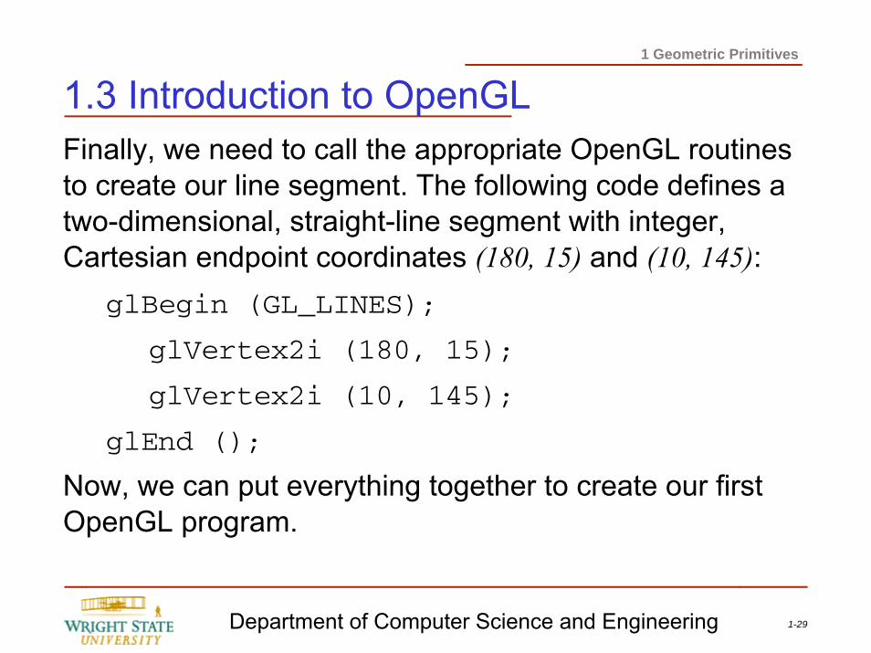
1.3 Introduction to OpenGLFinally, we need to call the appropriate OpenGL routines to create our line segment. The following code defines a two-dimensional, straight-line segment with integer, Cartesian endpoint coordinates (180, 15) and (10, 145):

glBegin (GL_LINES);

glVertex2i (180, 15);


glEnd ();

Now, we can put everything together to create our first OpenGL program.



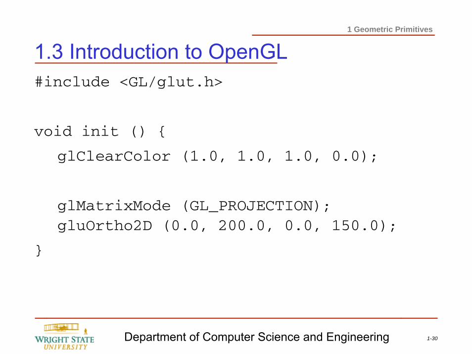
1.3 Introduction to OpenGL#include <GL/glut.h>

void init () {

glClearColor (1.0, 1.0, 1.0, 0.0);

glMatrixMode (GL_PROJECTION);gluOrtho2D (0.0, 200.0, 0.0, 150.0);

}



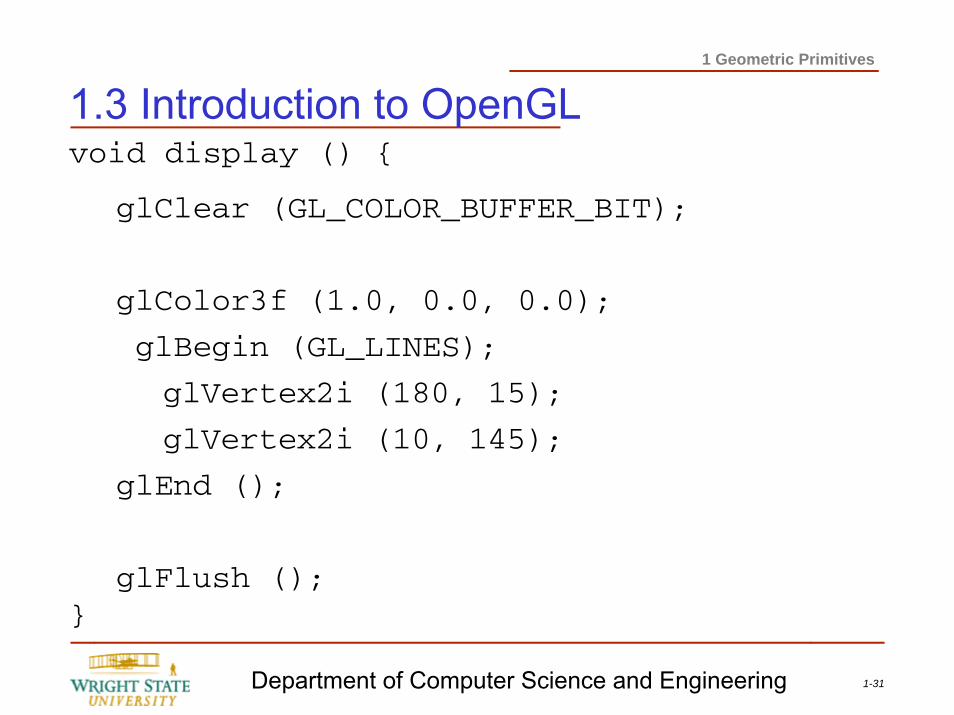
1.3 Introduction to OpenGLvoid display () {

glClear (GL_COLOR_BUFFER_BIT);

glColor3f (1.0, 0.0, 0.0);

glBegin (GL_LINES);



glEnd ();

glFlush ();}



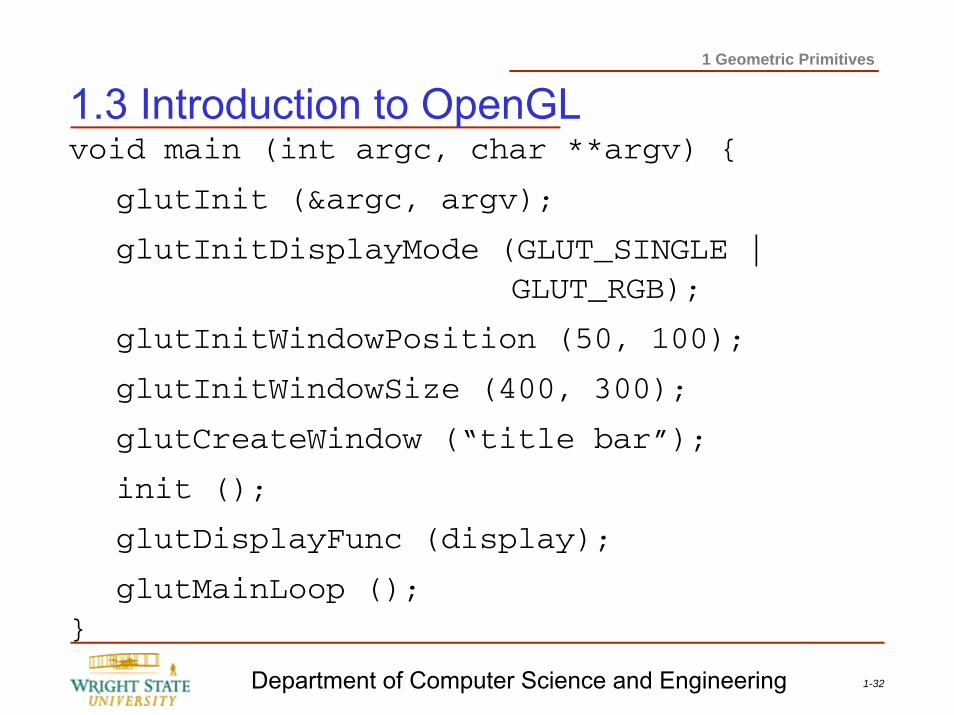
1.3 Introduction to OpenGLvoid main (int argc, char **argv) {

glutInit (&argc, argv);

glutInitDisplayMode (GLUT_SINGLE | GLUT_RGB);

glutInitWindowPosition (50, 100);

glutInitWindowSize (400, 300);

glutCreateWindow (“title bar”);

init ();

glutDisplayFunc (display);

glutMainLoop ();}



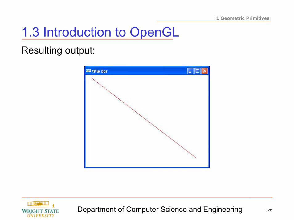
1.3 Introduction to OpenGLResulting output:



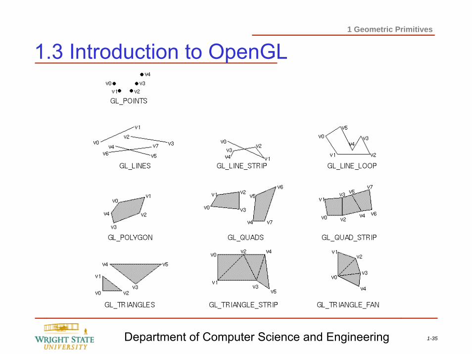
1.3 Introduction to OpenGLOpenGL supports several graphical primitives:

GL_POINTS GL_POLYGON

GL_LINES GL_TRIANGLES

GL_LINE_STRIP GL_TRIANGLE_STRIP

GL_LINE_LOOP GL_TRIANGLE_FAN

GL_QUADS

GL_QUAD_STRIP

Convenience functions exist for certain objects:glutSolidTetrahedron glutWiredTetrahedron

glutSolidCube glutWireCube

…



1.3 Introduction to OpenGL



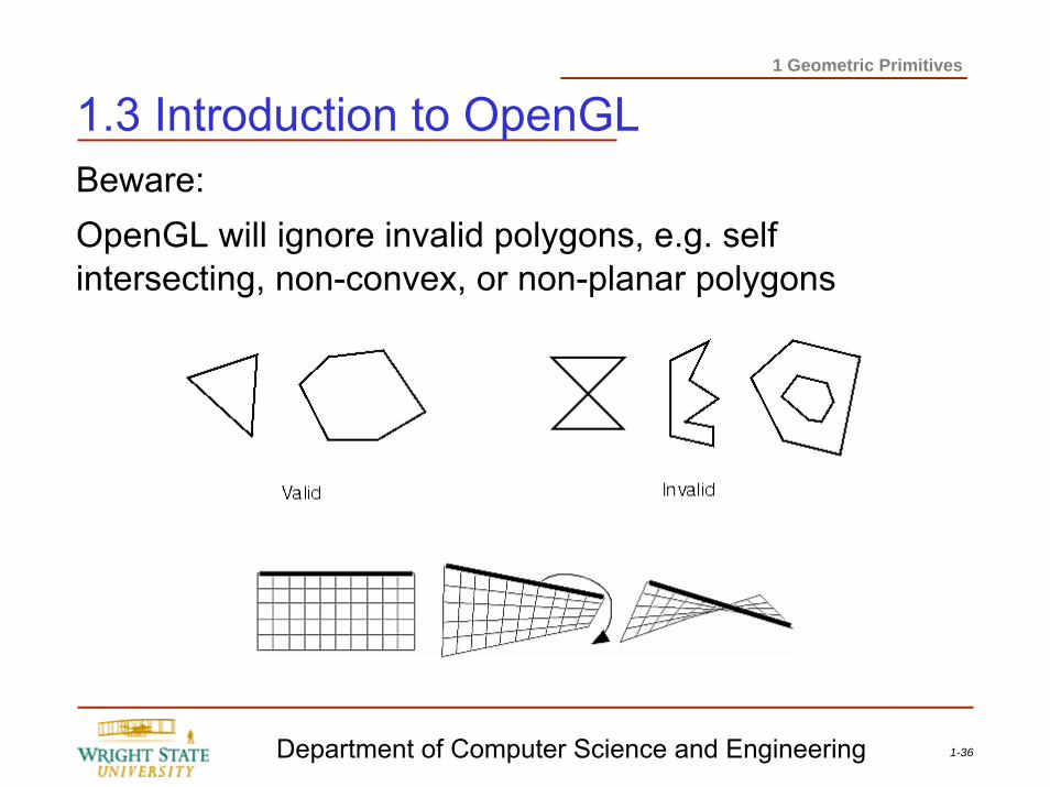
1.3 Introduction to OpenGLBeware: OpenGL will ignore invalid polygons, e.g. self intersecting, non-convex, or non-planar polygons



1.3 Introduction to OpenGLThere are basically four different ways to render geometric objects with OpenGL:• Direct rendering• Display lists• Vertex arrays• (Vertex buffer objects)



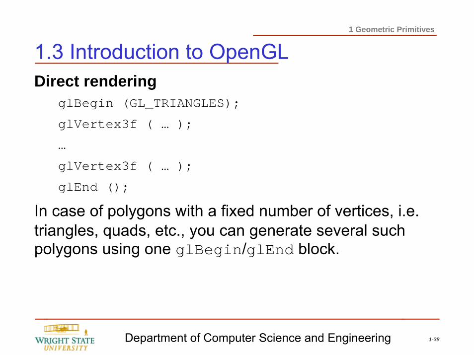
1.3 Introduction to OpenGLDirect rendering

glBegin (GL_TRIANGLES);

glVertex3f ( … );

…

glVertex3f ( … );

glEnd ();

In case of polygons with a fixed number of vertices, i.e. triangles, quads, etc., you can generate several such polygons using one glBegin/glEnd block.



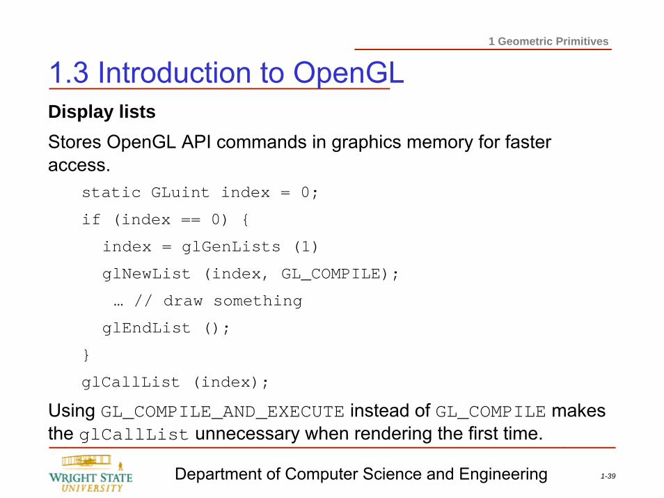
1.3 Introduction to OpenGLDisplay listsStores OpenGL API commands in graphics memory for faster access.

static GLuint index = 0;

if (index == 0) {

index = glGenLists (1)

glNewList (index, GL_COMPILE);

… // draw something

glEndList ();

}

glCallList (index);

Using GL_COMPILE_AND_EXECUTE instead of GL_COMPILE makes the glCallList unnecessary when rendering the first time.



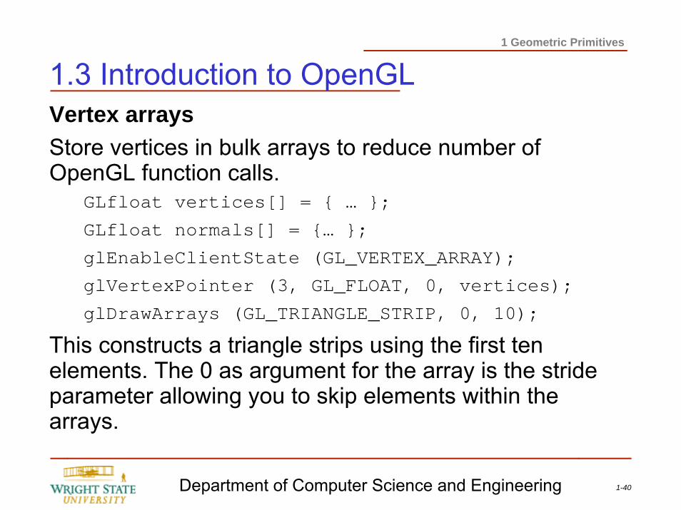
1.3 Introduction to OpenGLVertex arraysStore vertices in bulk arrays to reduce number of OpenGL function calls.

GLfloat vertices[] = { … };

GLfloat normals[] = {… };

glEnableClientState (GL_VERTEX_ARRAY);

glVertexPointer (3, GL_FLOAT, 0, vertices);

glDrawArrays (GL_TRIANGLE_STRIP, 0, 10);

This constructs a triangle strips using the first ten elements. The 0 as argument for the array is the stride parameter allowing you to skip elements within the arrays.



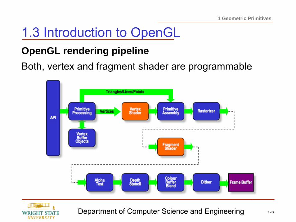
1.3 Introduction to OpenGLOpenGL rendering pipelineBoth, vertex and fragment shader are programmable



1.4 Rendering primitives on raster displaysThe raster display technology requires to brake down graphic primitives into pixels within the raster. This process is called rastering. This is usually done by the graphics hardware. It is, however, useful to understand how this process works in order to be able to achieve good graphics performance.In this subsection, we will discuss

– Rastering of straight lines, circles, ellipses, and polygons

– Antialiasing of lines and polygons



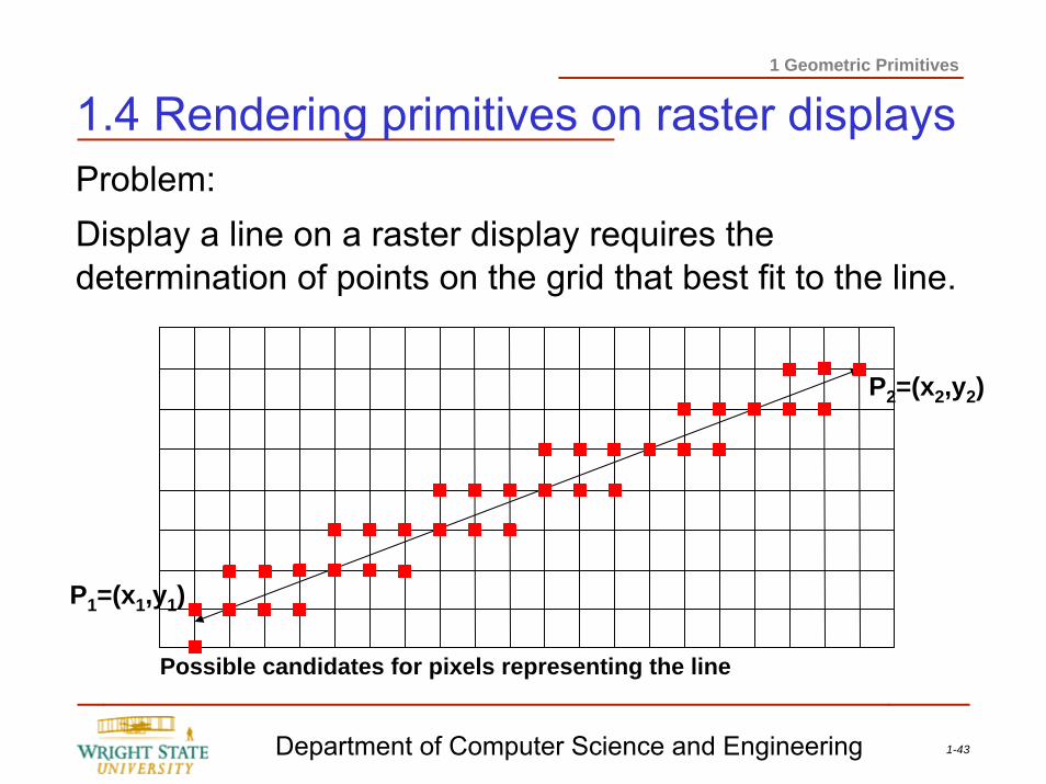
1.4 Rendering primitives on raster displaysProblem:Display a line on a raster display requires the determination of points on the grid that best fit to the line.

P1=(x1,y1)

P2=(x2,y2)

Possible candidates for pixels representing the line



1.4 Rendering primitives on raster displaysDesired properties:

– Line should appear straight– Line should appear with the same brightness everywhere– Algorithm should be fast– Algorithm should be portable to graphics hardware



1.4 Rendering primitives on raster displaysDDA algorithmThe digital differential analyzer (DDA) is a scan-conversion line algorithm based on calculating differences based on the slope of the line.A line can be described by the equation

y = m • x + bWithout loss of generality, we can assume 0 < m < 1. Otherwise we can mirror or interchange the coordinates as needed.Now, we need to compute the series of points (xk, yk), k=0,…,n that best describes the line.



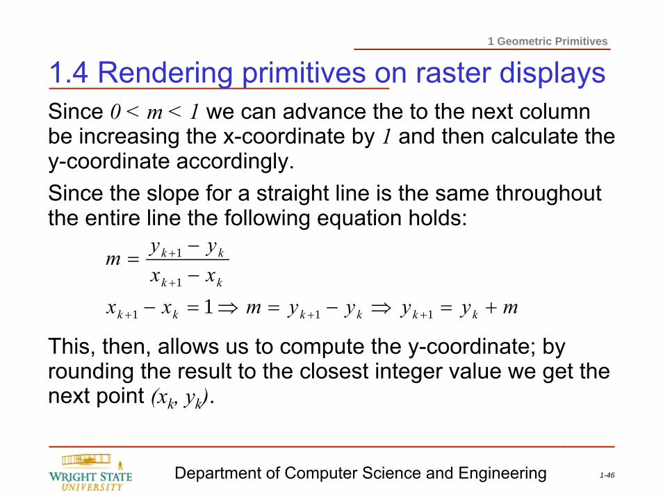
1.4 Rendering primitives on raster displaysSince 0 < m < 1 we can advance the to the next column be increasing the x-coordinate by 1 and then calculate the y-coordinate accordingly.Since the slope for a straight line is the same throughout the entire line the following equation holds:

This, then, allows us to compute the y-coordinate; by rounding the result to the closest integer value we get the next point (xk, yk).

myyyymxxxxyym

kkkkkk

kk

kk

+=⇒−=⇒=−−−

=

+++

+

+

111

1

1

1



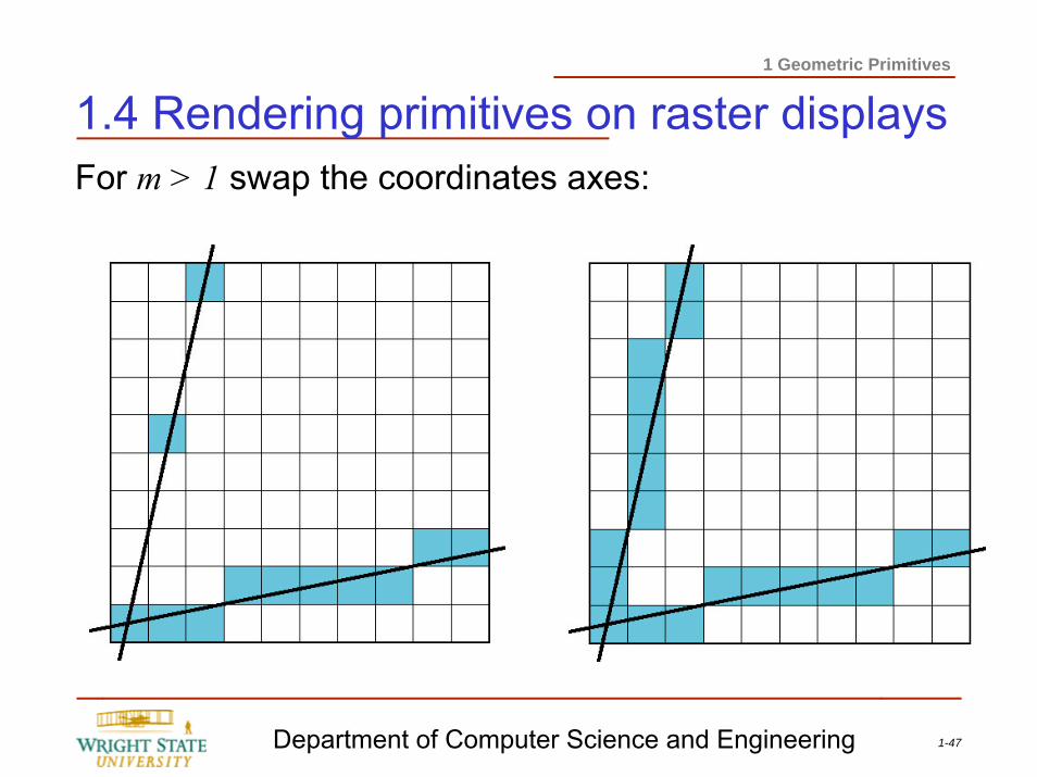
1.4 Rendering primitives on raster displaysFor m > 1 swap the coordinates axes:



1.4 Rendering primitives on raster displaysThe DDA algorithm easily can be extended to other graphics primitives, such as circles, ellipses, etc.The DDA line algorithm computes the coordinates for the next y-coordinate using floating-point numbers. Floating-point computations tend to be slower then integer computations. Hence, it is desirable to have an algorithm that is just based on integer coordinates, especially since the resulting pixel coordinates are represented as integer coordinates anyway.The Bresenham algorithm allows us to do just that.



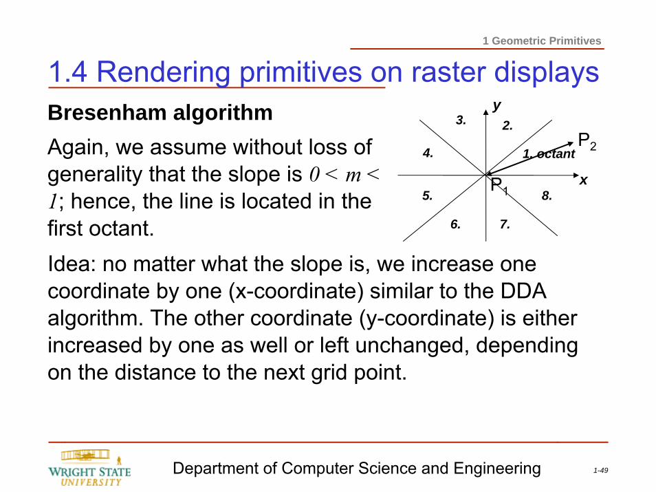
1.4 Rendering primitives on raster displaysBresenham algorithmAgain, we assume without loss of generality that the slope is 0 < m < 1; hence, the line is located in the first octant.

3.

4.

5.

6. 7.

8.

1. octantP2

x

y

P1

2.

Idea: no matter what the slope is, we increase one coordinate by one (x-coordinate) similar to the DDA algorithm. The other coordinate (y-coordinate) is either increased by one as well or left unchanged, depending on the distance to the next grid point.



1.4 Rendering primitives on raster displays

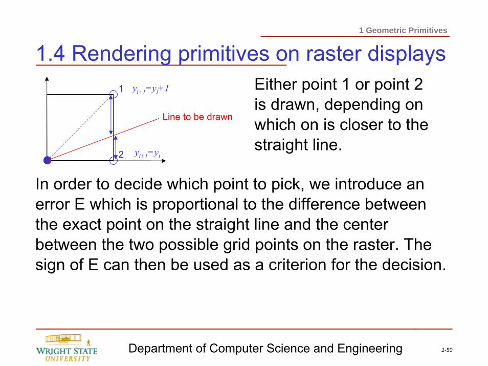
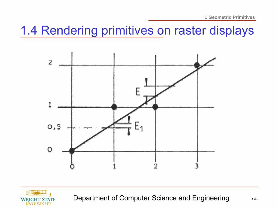
In order to decide which point to pick, we introduce an error E which is proportional to the difference between the exact point on the straight line and the center between the two possible grid points on the raster. The sign of E can then be used as a criterion for the decision.

Line to be drawn

1

2 yi+1=yi

yi+1=yi+1 Either point 1 or point 2 is drawn, depending on which on is closer to the straight line.



1.4 Rendering primitives on raster displays



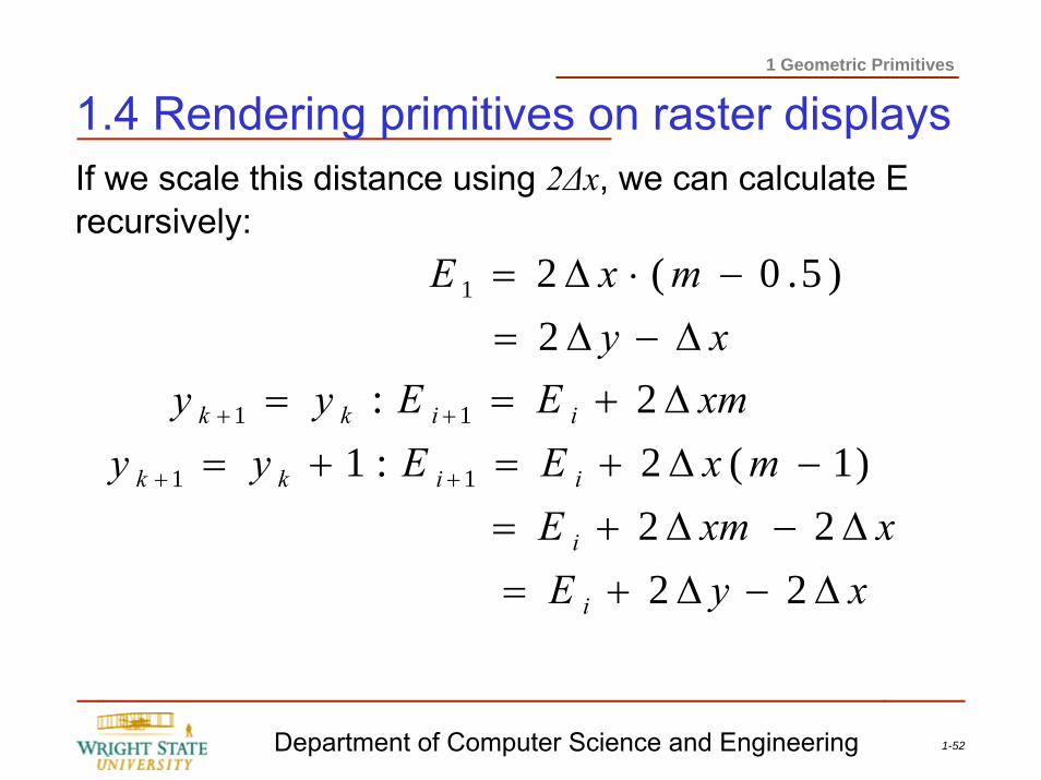
1.4 Rendering primitives on raster displaysIf we scale this distance using 2Δx, we can calculate E recursively:

2222

)1(2:1 2:

2 )5.0(2

11

11

1

xyExxmE

mxEEyyxmEEyyxy

mxE

i

i

iikk

iikk

Δ−Δ+=Δ−Δ+=

−Δ+=+=Δ+==Δ−Δ=−⋅Δ=

++

++



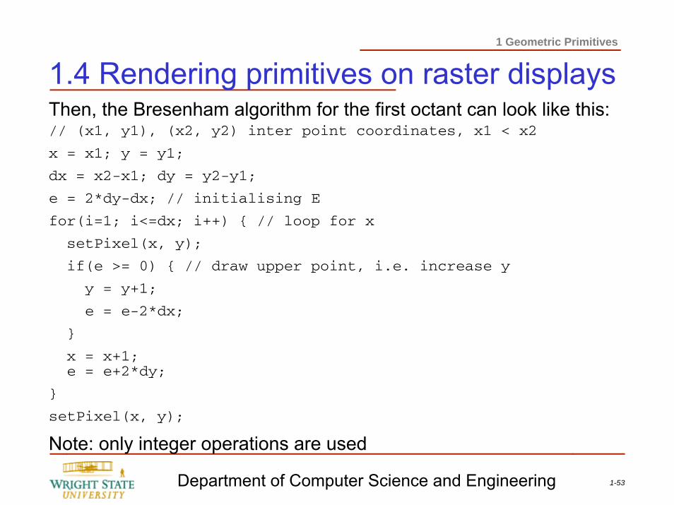
1.4 Rendering primitives on raster displaysThen, the Bresenham algorithm for the first octant can look like this:// (x1, y1), (x2, y2) inter point coordinates, x1 < x2

x = x1; y = y1;

dx = x2-x1; dy = y2-y1;

e = 2*dy-dx; // initialising E

for(i=1; i<=dx; i++) { // loop for x

setPixel(x, y);

if(e >= 0) { // draw upper point, i.e. increase y

y = y+1;

e = e-2*dx;

}

x = x+1;e = e+2*dy;

}

setPixel(x, y);

Note: only integer operations are used



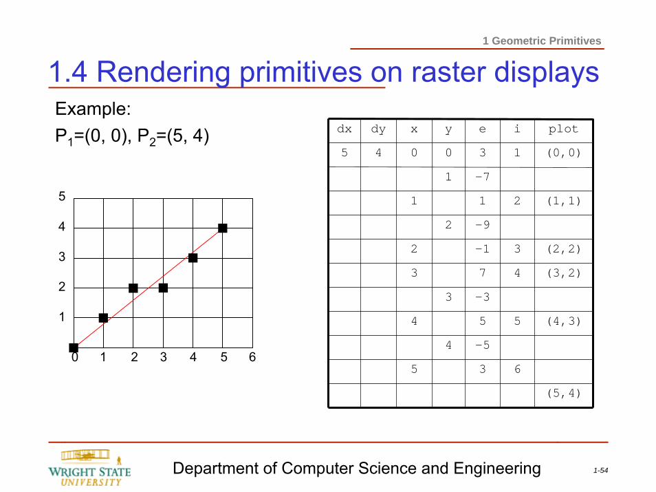
1.4 Rendering primitives on raster displaysExample:P1=(0, 0), P2=(5, 4)

(5,4)

635

(4,3)

(3,2)

(2,2)

(1,1)

(0,0)

plot

-54

554

-33

473

3-12

-92

211

-71

130045

ieyxdydx

0 1 2 3 4 5 6

1

2

3

4

5



1.4 Rendering primitives on raster displaysRastering circlesTo scan-convert circles based on a mathematical description can be quite expensive as we will see on the next slide.However, the basic principal of the Bresenham algorithm can be applied to other graphics primitives as well.For example, circles can be scan-converted for a raster display in a similar fashion. Of course, the error has to be computed differently as illustrated on the next slides.



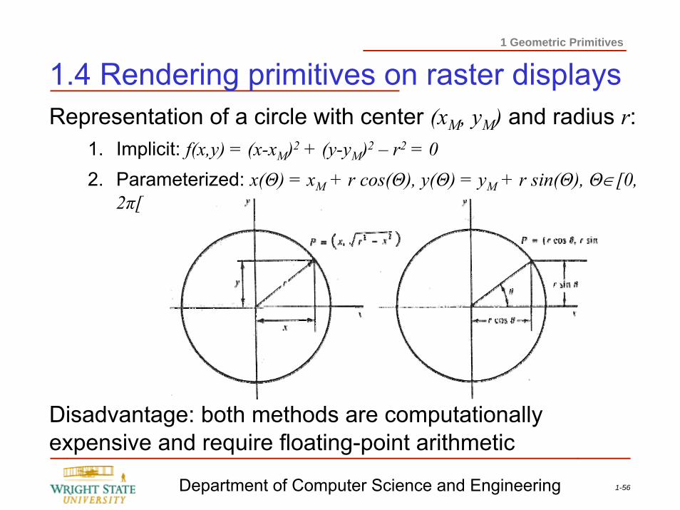
1.4 Rendering primitives on raster displaysRepresentation of a circle with center (xM, yM) and radius r:

1. Implicit: f(x,y) = (x-xM)2 + (y-yM)2 – r2 = 02. Parameterized: x(Θ) = xM + r cos(Θ), y(Θ) = yM + r sin(Θ), Θ∈[0,

2π[

Disadvantage: both methods are computationally expensive and require floating-point arithmetic



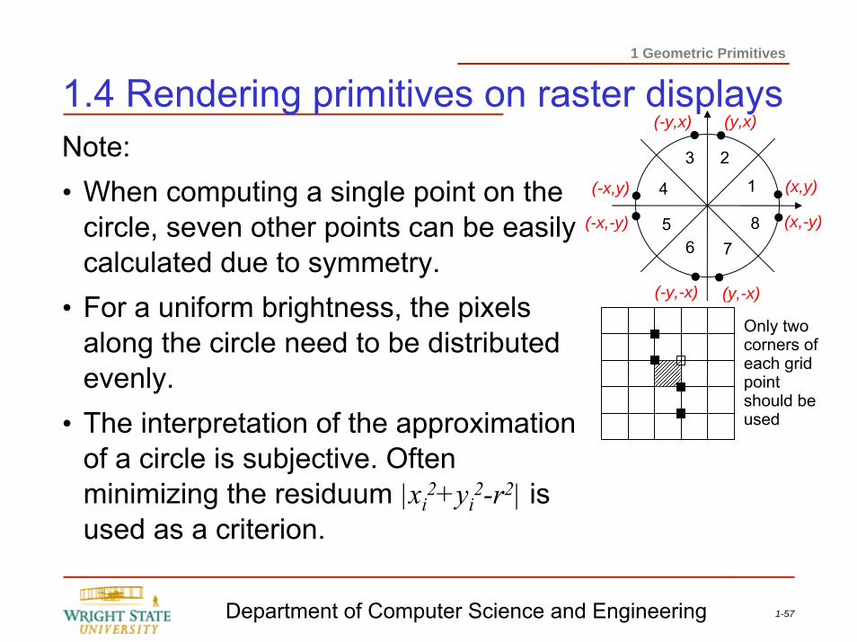
1.4 Rendering primitives on raster displaysNote:• When computing a single point on the

circle, seven other points can be easily calculated due to symmetry.

• For a uniform brightness, the pixels along the circle need to be distributed evenly.

• The interpretation of the approximation of a circle is subjective. Often minimizing the residuum |xi

2+yi2-r2| is

used as a criterion.

1

23

4

56 7

8

(x,y)

(y,x)(-y,x)

(-x,y)

(-x,-y)

(-y,-x) (y,-x)

(x,-y)

Only two corners of each grid point should be used



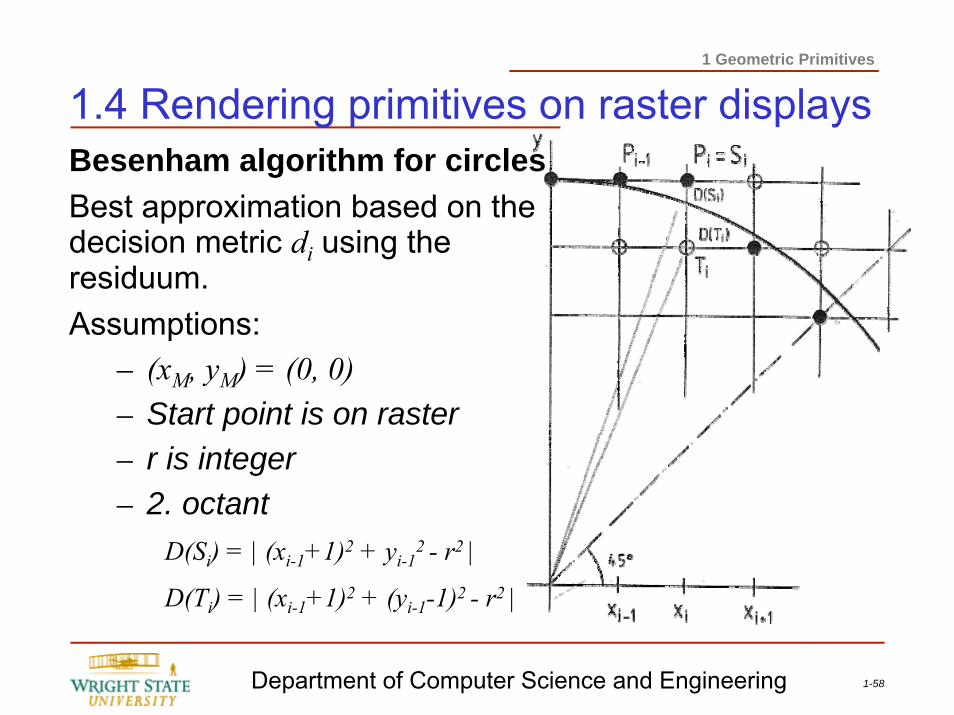
1.4 Rendering primitives on raster displaysBesenham algorithm for circlesBest approximation based on the decision metric di using the residuum.Assumptions:

– (xM, yM) = (0, 0)– Start point is on raster– r is integer– 2. octant

D(Si) = | (xi-1+1)2 + yi-12 - r2 |

D(Ti) = | (xi-1+1)2 + (yi-1-1)2 - r2 |



1.4 Rendering primitives on raster displaysThe decision metric di = D(Si) – D(Ti) measures the distance between the upper and lower raster point.For di > 0:

pick Pi = Ti as the next point, thus xi = xi-1+1, yi = yi-1-1For di < 0:

pick Pi = Si as the next point, thus xi = xi-1+1, yi = yi-1

Within the 2. octant the circle is monotonically decreasing, the slope is between 0 and -1. Therefore:(xi-1+1)2 + yi-1

2 - r2>0 and (xi-1+1)2 + (yi-1-1)2 - r2 < 0Thus: di = (xi-1+1)2 + yi-1

2 - r2 + (xi-1+1)2 + (yi-1-1)2 - r2



1.4 Rendering primitives on raster displaysdi = (xi-1+1)2 + yi-1

2 - r2 + (xi-1+1)2 + (yi-1-1)2 - r2

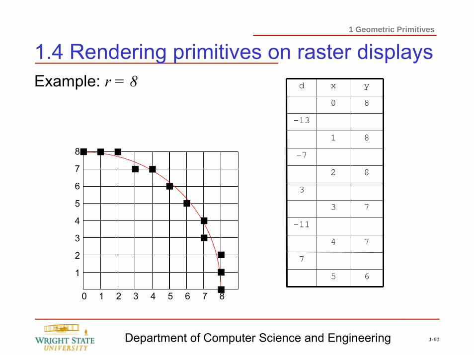
We, then, can compute di recursively:di+1 = di + 4 (xi-1 - yi-1) + 10 for di > 0di+1 = di + 4 xi + 2 for di ≤ 0with a start value of d1 = 3-2r (x0=0, y0=r)



1.4 Rendering primitives on raster displaysExample: r = 8

65

7

74

-11

73

3

82

-7

81

-13

80

yxd

0 1 2 3 4 5 6

1

2

3

4

5

6

7

8

87



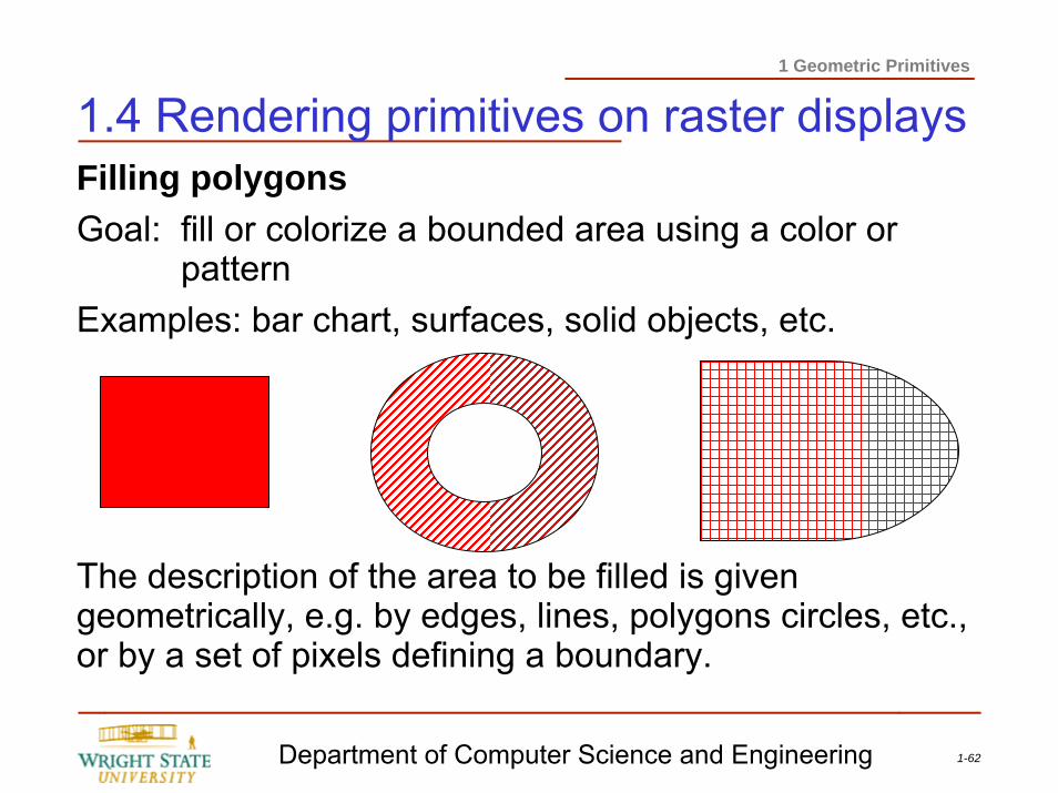
1.4 Rendering primitives on raster displaysFilling polygonsGoal: fill or colorize a bounded area using a color or

patternExamples: bar chart, surfaces, solid objects, etc.

The description of the area to be filled is given geometrically, e.g. by edges, lines, polygons circles, etc., or by a set of pixels defining a boundary.



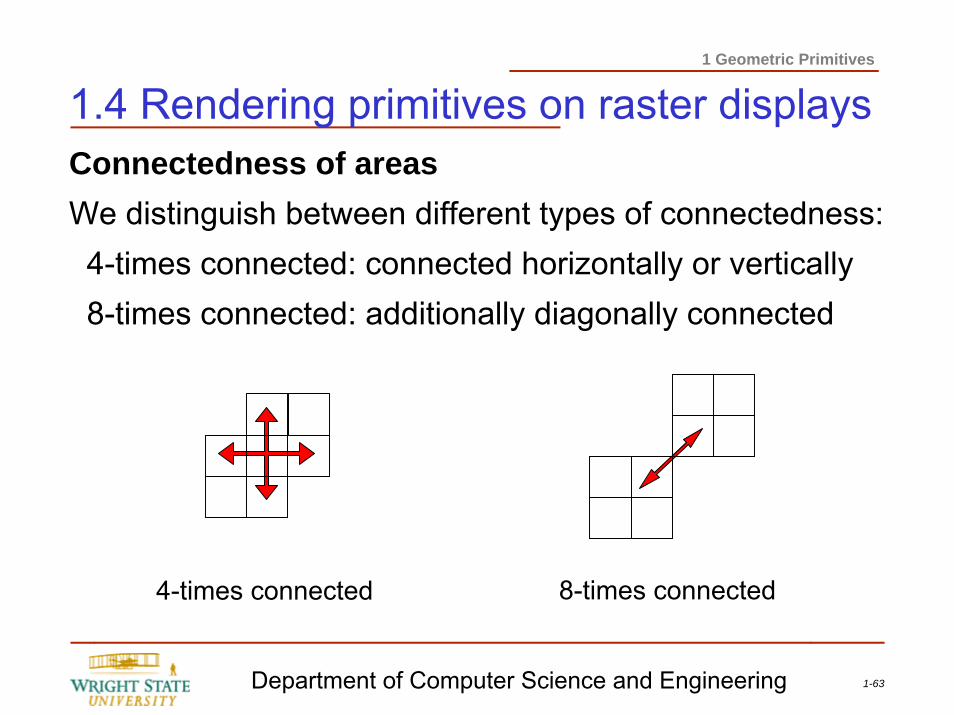
1.4 Rendering primitives on raster displaysConnectedness of areasWe distinguish between different types of connectedness:4-times connected: connected horizontally or vertically8-times connected: additionally diagonally connected

8-times connected4-times connected



1.4 Rendering primitives on raster displaysCommentsFilling algorithms designed for 8-times connected areas can also fill 4-times connected areas.Problem: 4-times connected areas with adjacent cornersFilling algorithms for 4-times connected areas cannot fill all 8-times connected areas.Techniques for rastering a polygon or an area:

– Scan-line methods– Seed fill methods– Hybrid methods



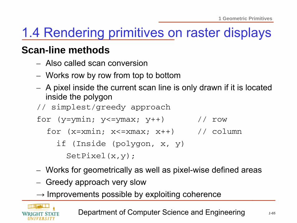
1.4 Rendering primitives on raster displaysScan-line methods

– Also called scan conversion– Works row by row from top to bottom– A pixel inside the current scan line is only drawn if it is located

inside the polygon// simplest/greedy approach

for (y=ymin; y<=ymax; y++) // row

for (x=xmin; x<=xmax; x++) // column

if (Inside (polygon, x, y)

SetPixel(x,y);

– Works for geometrically as well as pixel-wise defined areas– Greedy approach very slow→ Improvements possible by exploiting coherence



1.4 Rendering primitives on raster displaysScan-line methods (continued)The approach is based on scan-line coherence:Neighboring pixels are very likely to get the same intensity/color values assigned.→ The pixel characteristics, i.e. color/intensity values,

only changes where an edge of the polygon intersects the scan line, i.e. the part of the scan-line between two intersection points is either completely inside or completely outside of the polygon



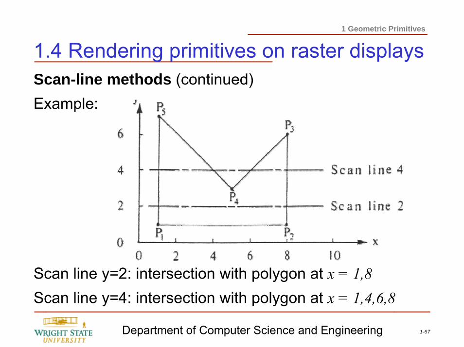
1.4 Rendering primitives on raster displaysScan-line methods (continued)Example:

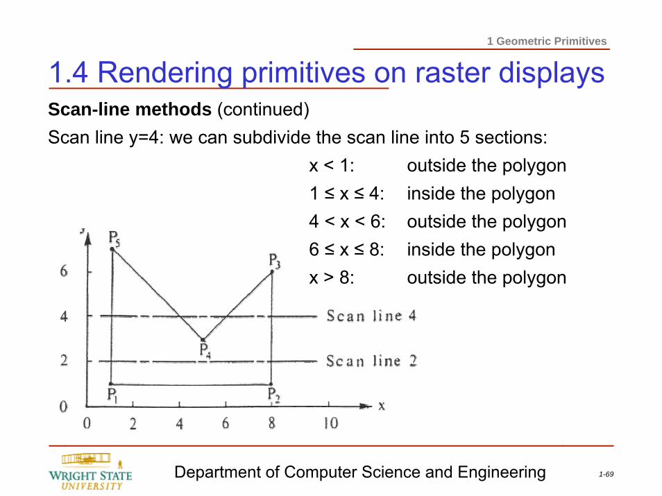
Scan line y=2: intersection with polygon at x = 1,8Scan line y=4: intersection with polygon at x = 1,4,6,8



1.4 Rendering primitives on raster displaysScan-line methods (continued)

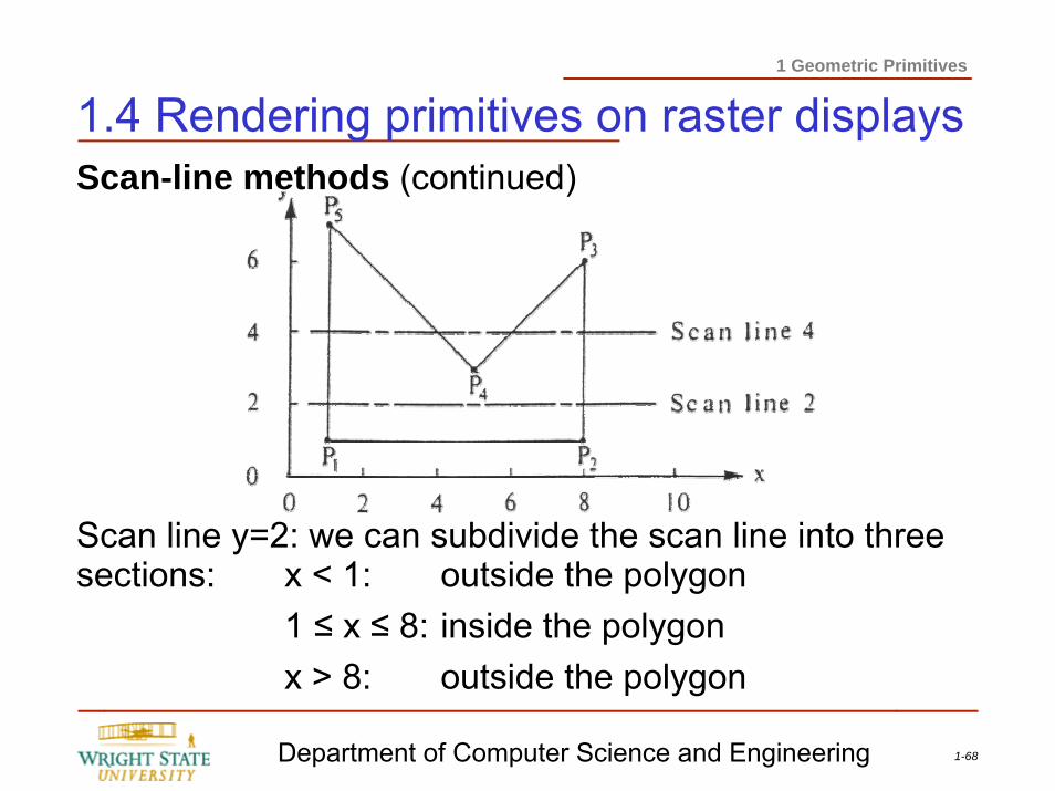
Scan line y=2: we can subdivide the scan line into three sections: x < 1: outside the polygon

1 ≤ x ≤ 8: inside the polygonx > 8: outside the polygon



1.4 Rendering primitives on raster displaysScan-line methods (continued)Scan line y=4: we can subdivide the scan line into 5 sections:

x < 1: outside the polygon1 ≤ x ≤ 4: inside the polygon4 < x < 6: outside the polygon6 ≤ x ≤ 8: inside the polygonx > 8: outside the polygon



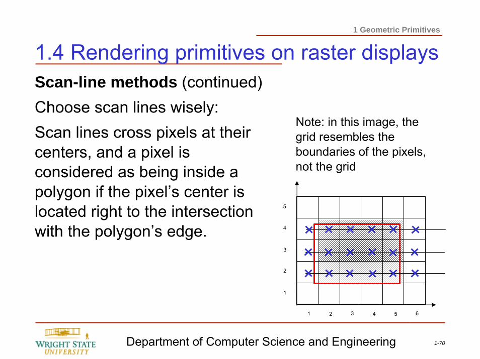
1.4 Rendering primitives on raster displaysScan-line methods (continued)Choose scan lines wisely:Scan lines cross pixels at their centers, and a pixel is considered as being inside a polygon if the pixel’s center is located right to the intersection with the polygon’s edge.

1 2 3 4 5 6

1

2

3

4

5

Note: in this image, the grid resembles the boundaries of the pixels, not the grid



1.4 Rendering primitives on raster displaysScan-line methods (continued)Problematic are singularities, i.e. locations where the scan line intersects with a vertex of the polygon.⇒ Consider local extremesLocal extremes: those y-values of the corner of the polygon where these values are greater or smaller than both vertices (with respect to the y-value) at the opposite side of the edge.Distinguish two cases:1. If the vertex a local extreme, the intersection counts twice2. If the vertex is no local extreme, the intersection counts

once only



1.4 Rendering primitives on raster displaysScan-line methods (continued)The simple ordered edge list algorithmMethod: pre-processing + scan conversiona) Preprocessing

Determine for every edge of the polygon the intersections with the scan lines at the pixel centers (e.g. using the Bresenham or other DDA algorithm); ignore horizontal edges.Store every intersection (x,y) in a list.Sort list from top to bottom, left to right.



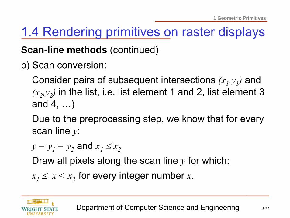
1.4 Rendering primitives on raster displaysScan-line methods (continued)b) Scan conversion:

Consider pairs of subsequent intersections (x1,y1) and (x2,y2) in the list, i.e. list element 1 and 2, list element 3 and 4, …)Due to the preprocessing step, we know that for every scan line y:y = y1 = y2 and x1 ≤ x2

Draw all pixels along the scan line y for which:x1 ≤ x < x2 for every integer number x.



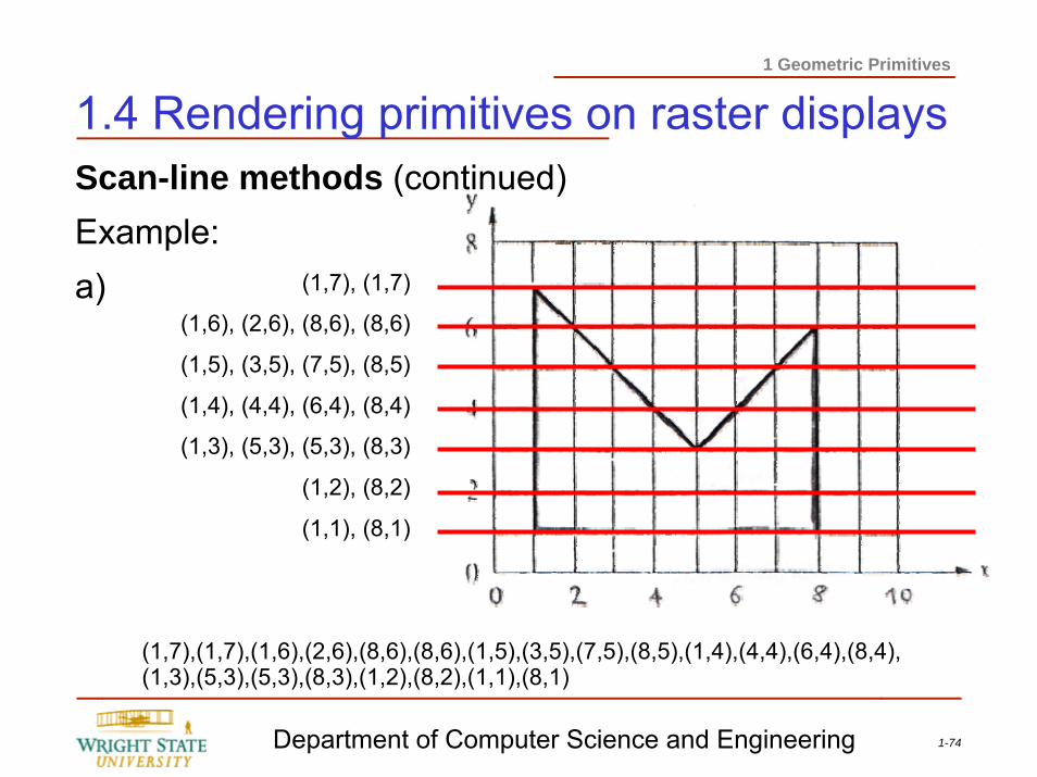
1.4 Rendering primitives on raster displaysScan-line methods (continued)Example:a) (1,7), (1,7)

(1,6), (2,6), (8,6), (8,6)

(1,5), (3,5), (7,5), (8,5)

(1,4), (4,4), (6,4), (8,4)

(1,3), (5,3), (5,3), (8,3)

(1,2), (8,2)

(1,1), (8,1)

(1,7),(1,7),(1,6),(2,6),(8,6),(8,6),(1,5),(3,5),(7,5),(8,5),(1,4),(4,4),(6,4),(8,4),(1,3),(5,3),(5,3),(8,3),(1,2),(8,2),(1,1),(8,1)



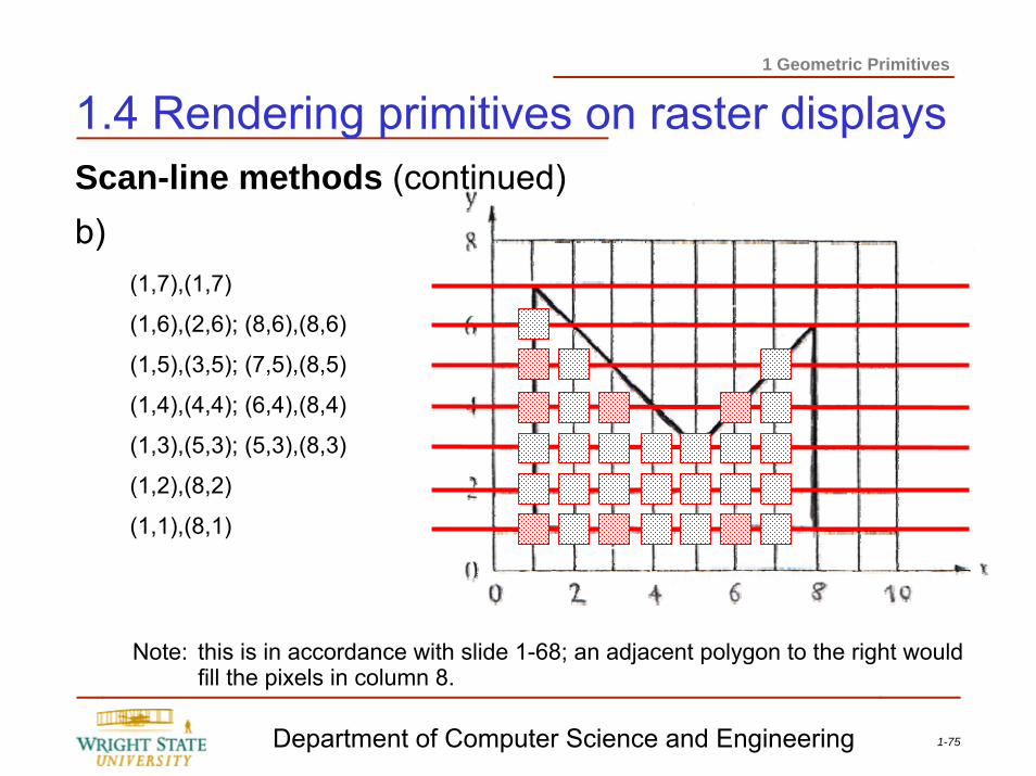
1.4 Rendering primitives on raster displaysScan-line methods (continued)b)

(1,7),(1,7)

(1,6),(2,6); (8,6),(8,6)

(1,5),(3,5); (7,5),(8,5)

(1,4),(4,4); (6,4),(8,4)

(1,3),(5,3); (5,3),(8,3)

(1,2),(8,2)

(1,1),(8,1)

Note: this is in accordance with slide 1-68; an adjacent polygon to the right would fill the pixels in column 8.



1.4 Rendering primitives on raster displaysSeed fill methodSeed fill methods fill the area bounded by the polygon starting from an initial pixel (seed) and are suitable for pixel-wise defined areas, hence also for raster displays.Usually, we differentiate between two differently defined areas:(i) Boundary fill algorithms

Input: initial pixel (seed), color of the boundary, fill color or patternAlgorithm: starting at the seed, neighboring pixels are colored until the boundary is reached (or an already colored pixel is encountered).



1.4 Rendering primitives on raster displaysSeed fill method (continued)(ii) Flood/interior fill algorithm

Input: initial pixel (seed), color of the pixels that are to be changed, fill color or patternAlgorithm: starting at the seed, neighboring pixels are colored using the fill color as long as the color is identical to the input color.



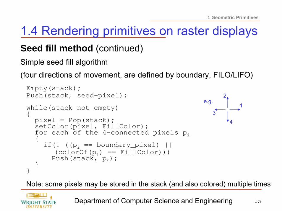
1.4 Rendering primitives on raster displaysSeed fill method (continued)Simple seed fill algorithm(four directions of movement, are defined by boundary, FILO/LIFO)Empty(stack);Push(stack, seed-pixel);

while(stack not empty){ pixel = Pop(stack);setColor(pixel, FillColor);for each of the 4-connected pixels pi{ if(! ((pi == boundary_pixel) ||

(colorOf(pi) == FillColor)))Push(stack, pi);

}}

1

2

34

e.g.

Note: some pixels may be stored in the stack (and also colored) multiple times



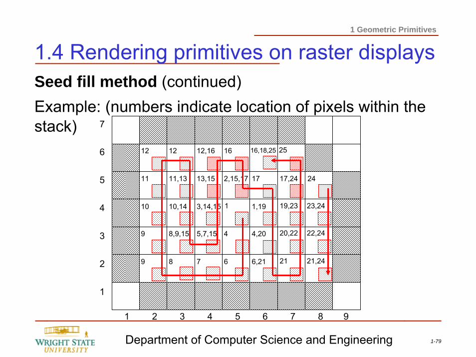
1.4 Rendering primitives on raster displaysSeed fill method (continued)Example: (numbers indicate location of pixels within the stack)

1

2

3

4

5

6

7

1 2 3 4 5 6 87 9

1,19

2,15,17

3,14,15

4

67

5,7,15

13,15

12,161212

11 11,13

10 110,14

8,9,159

9 8

16

6,21

4,20

17

16,18,25

17,24

25

19,23

20,22

21 21,24

22,24

23,24

24



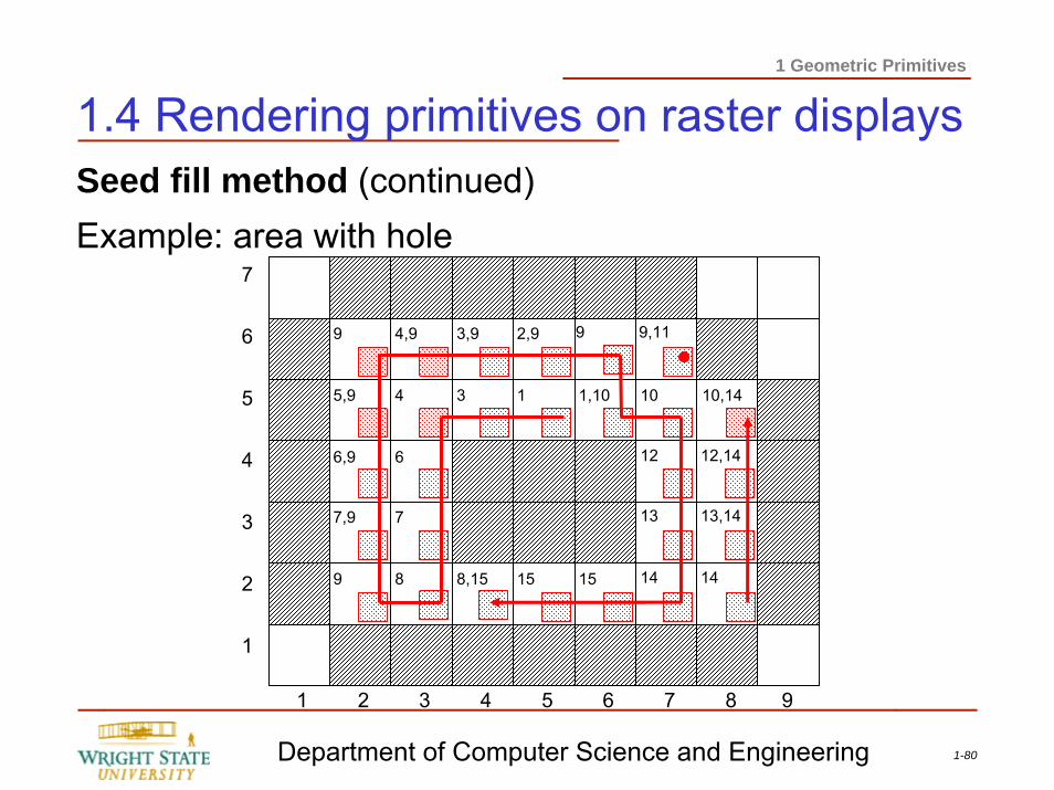
1.4 Rendering primitives on raster displaysSeed fill method (continued)Example: area with hole

1

2

3

4

5

6

7

1 2 3 4 5 6 87 9

1

158,15

3

3,94,99

5,9 4

6,9 6

77,9

9 8

2,9

15

1,10

9

10

9,11

12

13

14 14

13,14

12,14

10,14



1.4 Rendering primitives on raster displaysHybrid methodsHybrid methods follow the main principles of both scan line and seed fill methods⇒ Scan line seed fill algorithm



1.4 Rendering primitives on raster displaysAntialiasing (term from signal theory)Generally, aliasing effects are erroneous reconstruction of a (continuous) signal due sampling rate with a too low frequency (see also Nyquist theorem).The term aliasing in the area of computer graphics is used, besides visual effects resulting from the above (e.g. aliasing when rendering a checker board), to describe visual artifacts resulting from the process of scan conversion. (e.g. stair casing when drawing diagonal lines).We distinguish between local and temporal aliasing (e.g. a wheel that appears to rotate backwards).



1.4 Rendering primitives on raster displaysAntialiasing (continued)Anti-aliasing methods are techniques (e.g. over-sampling, filtering) that try to minimize the aliasing effect.Eliminating the aliasing effect is often not possible (already from a theoretical point of view).For aliasing effects resulting from scan conversion algorithms, the anti-aliasing method is also called “edge smoothing”.



1.4 Rendering primitives on raster displaysAntialiasing (continued)Aliasing artifacts in computer graphics• Texture artifacts (e.g. checker board)• Stair casing artifacts when rastering curves ⇒ jagged

lines• Disappearance of objects which are smaller than a

pixel• Disappearance of small, skinny objects• Loss of detail in complex images• “Flipping” small objects during motion/animation



1.4 Rendering primitives on raster displaysAntialiasing (continued)

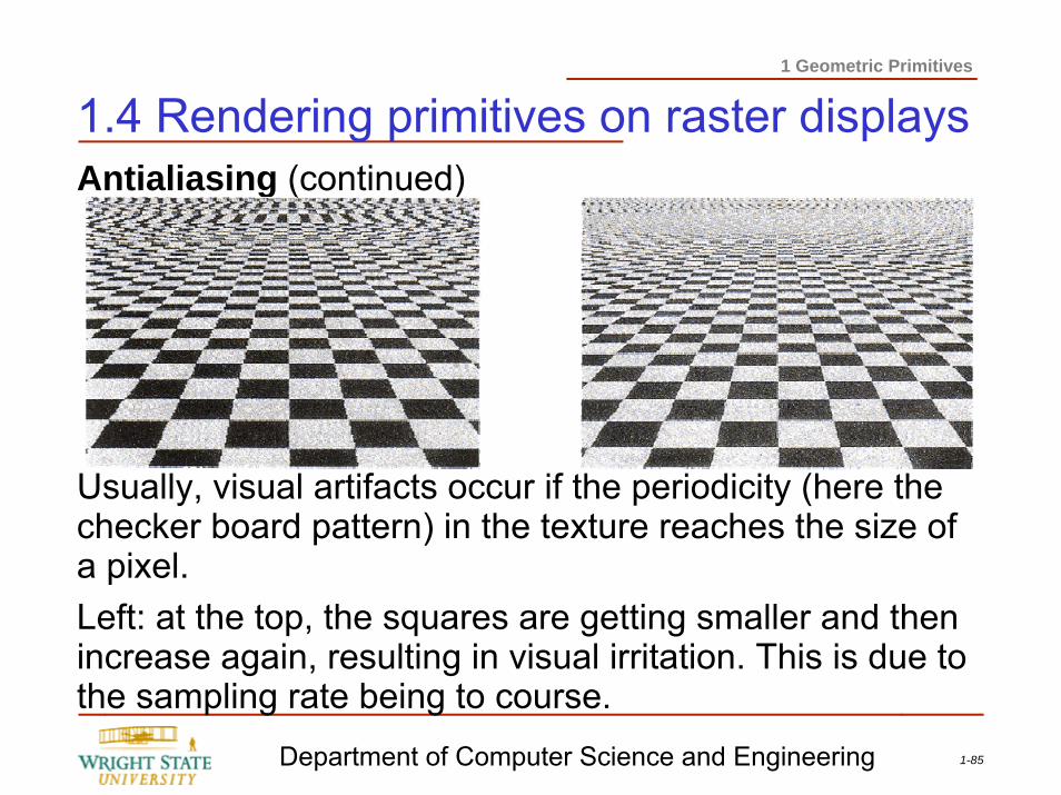
Usually, visual artifacts occur if the periodicity (here the checker board pattern) in the texture reaches the size of a pixel.Left: at the top, the squares are getting smaller and then increase again, resulting in visual irritation. This is due to the sampling rate being to course.




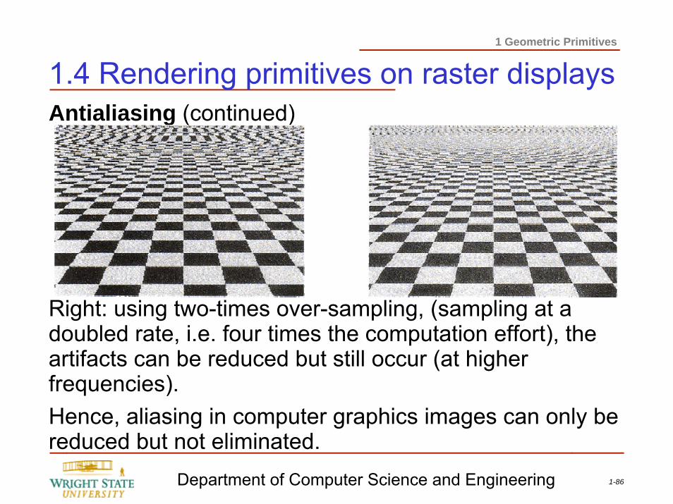
Right: using two-times over-sampling, (sampling at a doubled rate, i.e. four times the computation effort), the artifacts can be reduced but still occur (at higher frequencies).Hence, aliasing in computer graphics images can only be reduced but not eliminated.



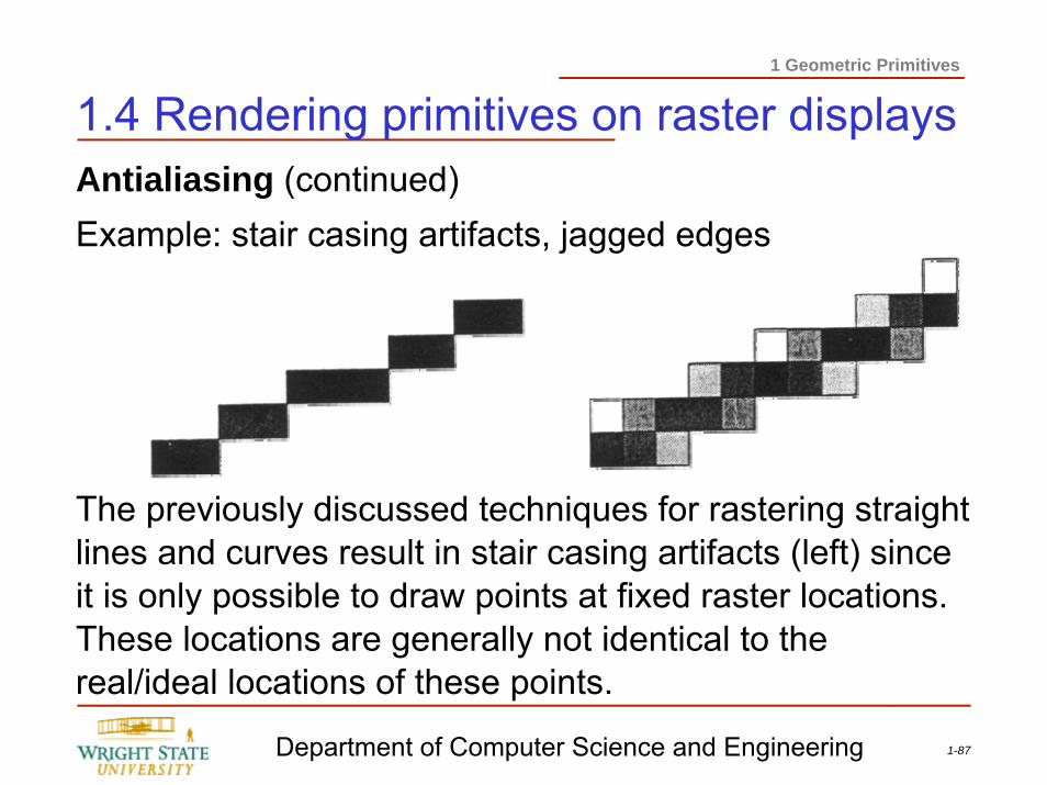
1.4 Rendering primitives on raster displaysAntialiasing (continued)Example: stair casing artifacts, jagged edges

The previously discussed techniques for rastering straight lines and curves result in stair casing artifacts (left) since it is only possible to draw points at fixed raster locations. These locations are generally not identical to the real/ideal locations of these points.



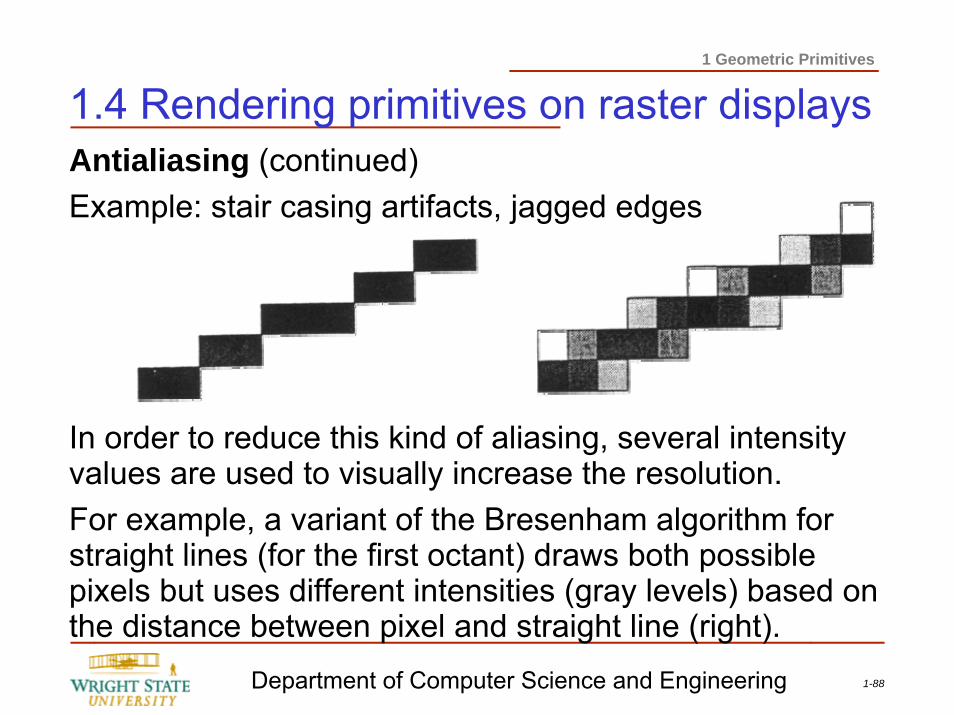
1.4 Rendering primitives on raster displaysAntialiasing (continued)Example: stair casing artifacts, jagged edges

In order to reduce this kind of aliasing, several intensity values are used to visually increase the resolution.For example, a variant of the Bresenham algorithm for straight lines (for the first octant) draws both possible pixels but uses different intensities (gray levels) based on the distance between pixel and straight line (right).



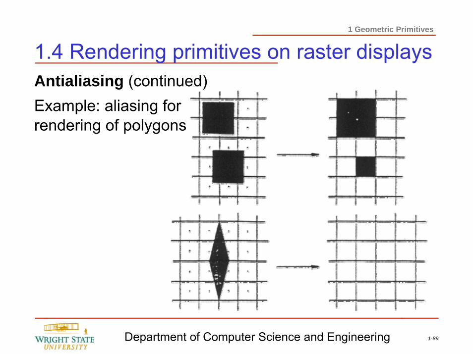
1.4 Rendering primitives on raster displaysAntialiasing (continued)Example: aliasing for rendering of polygons



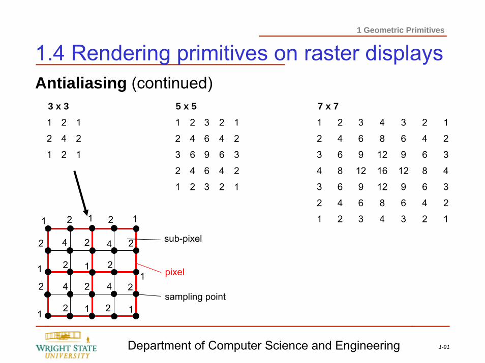
1.4 Rendering primitives on raster displaysAntialiasing (continued)A simple, global anti-aliasing can be achieved by applying the over-sampling, also known as super-sampling, to the entire image.Every pixel is computed at a higher sampling rate compared to the image resolution. The gray value or color value for that pixel is then determined as the weighted average of all its sub-pixel values.This approach is equivalent to a filtering (see digital signal processing for the theoretical basis).The following filter kernels are commonly used:




121

242

121

3

6

9

6

3

2

4

6

4

2

363

242

121

242

121

4

8

12

16

12

8

4

3

6

9

12

9

6

3

36963

481284

3

6

9

6

3

2

4

6

4

2

363

242

121

242

121

3 x 3 5 x 5 7 x 7

pixel

sub-pixel

sampling point

1 1 1

1

1 1 1

11

2

2 2 2

2

2

2

2 2

2

2

2

4 4

4 4



1.4 Rendering primitives on raster displaysAntialiasing in OpenGLIn order to use antialiasing when rendering points or lines you have to enable this feature in OpenGL first:

glEnable (GL_POINT_SMOOTH);

glEnable (GL_LINE_SMOOTH);

To disable antialiasing use the corresponding function call:

glDisable (GL_POINT_SMOOTH);

glDisable (GL_LINE_SMOOTH);



1.4 Rendering primitives on raster displaysAntialiasing in OpenGL (continued)To choose between quality or performance you can give OpenGL a hint accordingly:

glHint (GLenum target, GLenum hint);

where the following target parameters are available:GL_POINT_SMOOTH_HINT

GL_LINE_SMOOTH_HINT

GL_POLYGON_SMOOTH_HINT

and the following hints:GL_FASTEST, GL_NICEST, GL_DONT_CARE



1.4 Rendering primitives on raster displaysAntialiasing in OpenGL (continued)When using the RGBA mode (specified when initializing the display using glutInitDisplayMode) you need to specify the blending function as well. Most likely, you want to use the parameters GL_SRC_ALPHA and GL_ONE_MINUS_SRC_ALPHA to specify the blending function:

glEnable (GL_BLEND);

glBlendFunc (GL_SRC_ALPHA, GL_ONE_MINUS_SRC_ALPHA);

Documents

1 Geometric Primitives Chapter 1 - avida.cs.wright.edu