1

Geoinformatics Department, Palacky University Olomouc

Dr. Maik Netzband

Urban Remote Sensing and Landscape Metrics

1st StatGIS conference: 19.11.2013

2

Urban Remote Sensing and Geomatics

A city is characterised by its heterogeneity – in space and time

In the field of remote sensing and the applied data there are different sensors and scales selected dependent on the goal of the analysis

Unmodified and dynamically developing areas are closely intertwined in a city

In addition, a dynamic suburban and peri-urban environment with a manifold of interdependencies with the city exists

Spatial heterogeneity and a spatially limited , temporal dynamics are challenges for the monitoring and the analyse of remotely sensed data and digital Geoinformation datasets

3

Indicators for the urban environment Natural Environment:

Soil / groundwater: degree of imperviousness, risk of contamination

Climate / air: thermal stress, circulation

Green spaces: quantity and location, biodiversity, network of green spaces

Built-up Environment:Energy supply: Energy requirements / availability, energy consumption

Waste disposal: Quantity, collection, compost, recycling

Water management: needs, water treatment , rain water retention

Urban built-up structure: land use distribution and composition, densification and

urban land use potentials, building structure, state (quality) of buildings,industrial plants

Mobility structure: motorised, non-motorised people in streets, public transport

Social Environment:

Housing: housing supply, demolition, empty housing

Population: age structure, marital status, ♀/♂ , proportion of foreigners, income

Socio cultural structure: socio cultural infrastructure, supply with

goods and services, green spaces, quality of neighborhood environment

4

Methodological Background

Vegetation-Imperviousness-Soil (V-I-S) Modell after Ridd (1995)

Based on classification

Approach valid in general, but not transferable to any cities

Per

cent

Impe

rvio

usne

ss Percent S

oil

Percent Vegetation100

0

100

00

100LawnBare soil

CBD

Covercrops Forest

Rowcrops

Range- land Desert

Low density residentíal

Medium density residentíal

High density residentíal

Light industry

Heavy industry

Vegetation Soil

Imperviousness

Imperviousness as a kind of „paramount“ indicator for a variety of processes

5

1 : 100 000 - 1 : 50 000

1 : 25 000 - 1 : 15 000

1 : 10 000 - 1 : 5 000

20 – 30 m

10 – 15 m

1 – 5 m

urban entity= image set ofurban structures

urban structure= configurationof single elements

single structureelement (house,street,garden)

Pixel = smallest unitof on imagery depen-dent on spatialresolution. It cancontain one object or parts of objects

imagery /photography

classified image

0,20 – 1 m1 : 1 000 - 1 : 5000

Spatial resolution

Chara

cteri

sati

on G

enera

lisatio

n

Scale-dependent analyses exemplified for urban remote sensing studies

Modified after Puissant & Weber 2002

6

Scale-dependency: different sensors, resolutions, semantics

Landsat-5-TM [30 m]

05-Sept-2005Spot-5-XS [10 m]

07-Sept-2005

Urban structure:

Inner urban differentiation ▪ Amount, intensity, axes of infrastructure

Different building structures, densities ▪ Amount and structure of vegetation

Four Local Districts in the City of Leipzig

CIR photograph [40 cm]21-Juni 2005

• The ecosystem approach: fluxes of energy, matter and species.

• The patch dynamic approach: creation of the spatial heterogeneity within landscapes and how that influences the flow of energy, matter, etc. across the landscape.

• Spatially focused approach of patch dynamics (Pickett et al. 1997): urban landscape is a mosaic of biotic and abiotic patches within a matrix of infrastructure, social institutions, cycles and order.

• Spatial heterogeneity within an urban landscape has both natural and human sources.

Two ecological approaches to understand and manage the dynamics of urban and urbanizing ecosystems

• Analysed satellite image data is a very useful instrument offering the

information needed:

• continuous land-cover information,

• quasi-recent to retrospective (back to the 1970’s )

• reasonable price, i.e. for monitoring purposes

• Digital image processing and landscape metrics software can ‘sharpen’

information contained in the raster-based image structure:

• - texture

• - shape

• - neighbourhood

• Show public decision makers the necessity of regional concerted

actions and to be able to regulate the process (‘spatial map aha

effect’).

Remote Sensing and Landscape Metrics

9

Leipzig

Hanover

Trees, Forest Allotments and Backyard Gardens

IRS 1C Satellite Image Data -Classified Vegetation Cover

10

Configuration of green spaces

Netzband & Banzhaf, 2000

11

Patch density (#/100 ha)

0

5

10

15

20

1830_GR_Ost 1930_GR_Ost 1998_GR_Ost

Wald Grünland Standgew ässer Flüsse lineare Grünstruktur

Edge density (m/ha) of selected features (from TE)

0

10

20

30

40

50

60

70

1830_GR_Ost 1930_GR_Ost 1998_GR_Ost

Wald Grünland Standgew ässer Flüsse lineare Grünstruktur

Landscape metrics for the „Green Belt“ of Leipzig

■ PD equals the number of patches of the corresponding patch type (NP) divided by total landscape area, multiplied by 10,000 and 100 (to convert to 100 hectares).

■ facilitates the comparison of landscapes at different time slots

■ strongest decrease of shrubs / smaller trees patches in the 10-15 km zone

■ ED equals the sum of the lengths of all edge segments involving the corresponding patch type, divided by the total landscape area, converted to hectares.

■ decrease of edge lengths in the peri-urban area of the city

Netzband & Kirstein, 2001

Habitat Suitability Index (Shape Complexity

for Arable Land in Helsinki (1950-1998)

‘Green Edge Index’ for Urban Fabric

in Dublin (1956-1998) - how much of a region’s urban fabric

is adjacent to (i.e. has an edge with) vegetated areas.

Indicators on the basis of remotely sensed data

ASTER Land Cover Classification for Phoenix

Suite of landscape metrics available (FRAGSTATS); Class Area, Edge Density, Mean Shape Index, Interspersion and Juxtaposition Index.

Metrics calculated on 1 x 1 km grid to allow comparison of results between urban centers and comparison with other datasets such as MODIS.Stefanov and Netzband,

RSE, 2005

Landscape Characterization of Urban Centers

(Stefanov and Netzband, 2005)iew)

Landscape Metric Results for Phoenix

• Capital region of Andhra Pradesh State

• It spreads over an area of 1279 km²

• Urban population:

• increased by 41.57% as against 43% of the total Andhra Pradesh state and 36% of total country.

• just 0.44 million in 1901

• after India’s independence in 1947 1.13 million,

• up-to 3.6 million by 2001.

• Climate:

• hot semi-arid moist with dry summers maximum temperature 40ºC and mild winters minimum temperature up-to 15ºC with average rainfall of about 75 cm

Fig. 1 Location of study area Hyderabad

Andhra Pradesh

Rahman et al, 2009

Case study Hyderabad/Secunderabad

- In the North of Hyderabad

Hussain Sagar lake provides

water for the growing urban

population

- further expansion of this twin

city is mainly in the North

which is the new part called

Secundarabad, so the city

gradually expanded to an area

of 179 Km².

Physical expansion of Hyderabad

- Two basic data layer i) ward-wise map and ii) land use map.

- Land use/land cover map prepared for 1971 from topographical sheet at a scale of 50,000, for 1989 and 2001 from Landsat TM and ETM+ and for 2005 IRS P6 data

- NRSA 1995 classification scheme was used for major land use classes – see below...

- SoI toposheet of 1971 was geo-referenced and then digitized for the six major land use classes and that was used as a base map.Level I Level II 1. Built up land Residential, Government offices, educational

Institutions, recreational and cantonment 2. Water bodies River, streams, canals, lakes and reservoirs 3. Agricultural lands Cultivated lands and fallow lands 4. Forests Dense forest, degraded forests and plantation 5. Others Quarry, open urban areas and

To study the urban growth...

- Rate of development of land in the Hyderabad-Secundrabad region is far outstripping the rate of population growth.

- Implies that the land is consumed at excessive rates and probably in unnecessary amounts as well.

- Per capita consumption of land has increased steadily over three and half decades.

174%

124%

0

20

40

60

80

100

120

140

160

180

Builtup Vs Population Growth

Builtup change 1971-2005 Population Growth 1971-2001

Comparing built-up vs. population of Hyderabad

- 1971 total entropy value 0.627 and it increased to 0.918 in 2005 this

means that the expansion of Hyderabad has occurred at a fast rate in

the fertile fringe areas.

- Compact distribution and vertical development of built up entropy value (ranges

from 0 to log n) closer to 0

• Distribution very dispersed closer to log n.

• High value of entropy indicates the occurrence of urban growth in that particular

region.

Years Built-up Area (km²)

Increase in built-up area (in %)

Entropy value (En)

Entropy change (∆E)

1971 135 Base year 0.627 Base year 1989 214 58.52

(71/89) 0.712 13.6%

(71/89) 2001 288 34.58

(89/01) 0.794 26.6%

(89/01) 2005 370 28.47

(01/05) 0.918

29.1% (01/05)

Results show that...

- Built up area increased

almost in all wards of the city

but areas in the north-west

of the city (7-11) maximum

increase in the built-up area

- The four zones NW of

Hyderabad highest growth

rates, entropy value

increased from 0.409 in 1971

to 0.66 in 2005

- Reason: new township has

come up i.e. Hi-Tech city, a

hub of computer software.

Results also show...

22

Land coverArea 1989

[km²]

Area 2000

[km²]

In-

/Decrease

[%]

Area 2002

[km²]

In-

/Decrease

[%]

Area 2005

[km²]

In-

/Decrease

[%]

Urban area 102,9 174,5 69,5 291,0 66,8 522,1 79,4

Vegetation 485,2 289,7 -40,3 398,1 37,4 302,7 -24,0

Farmland 1066,2 1223,4 14,7 978,0 -20,1 809,6 -17,2

Water bodies 166,1 167,4 0,8 189,5 13,2 194,1 2,4

0%

20%

40%

60%

80%

100%

WaterbodiesFarmlandUrban Area

1989 200520022000

Change in land coverage for the period 1989 - 2005

23

20 km

20 km

Comparison HCMC - Hyderabad

1 2 3 4 5 6 7 8 9 10 11 12 13 14 15 16 17 18 19 200

10

20

30

40

50

60

70

80

90

100HCMC 1989

HCMC 2001

HCMC 2002

HCMC 2005

Ring radius - distance to the city centre [km]

Urb

an

De

nsi

ty G

rad

ien

t [%

]

• eGeopolis/Indiapolis – Digitization of Indian urban agglomerations – Author: French Insitute of Pondicherry

• Digitization on basis of Google Earth satellite image data

• The second step (2010-2012) consists of the exhaustive cartography of all Indian

settlements (>5000 inhabitants) and agglomerations, and in preparing the update of the census of 2011

Inde_1872_2001.gif

Inter urban comparisons - Concept

Agglomerations of

more than 20,000

inhabitants

Variation 1991 - 2001

• Creation of a raster grid of 5*5 km

• Delineation of rectangular ring zones with

raster grid elements in 5km distances starting

from a defined center grid element

• Calculation of digitized urban ‚footprint‘ within

the grid elements

• Statistical Analysis of urban agglomerations

Inter urban comparisons - Methodology

Delhi

Hyderabad

Kolkata

Bangalore

eGeopolis/Indiapolis – Test areas with 5km grid

eGeopolis/Indiapolis - Bangalore and Kolkata with 5km grid

• All start at similar high density level

• MC Delhi and Kolkata show higher values in increasing distance and slower decrease, higher variation (SD) than emerging MC Hyderabad and Bangalore

Mean Values

0

0,2

0,4

0,6

0,8

1

1,2

5km

10km

15km

20km

25km

30km

35km

40km

45km

50km

Delhi

Kolkata

Hyderabad

Bangalore

Standard Deviation

0

0,05

0,1

0,15

0,2

0,25

0,3

0,35

0,4

0,45

Delhi

Kolkata

Hyderabad

Bangalore

Inter Urban Comparisons - Results

• MC higher Majority values overall

• Minority varies a lot in the closer fringe areas, ‚stabilize‘ in the outer areas with higher values for the MC, lower for the EMC

Majority

0

0,2

0,4

0,6

0,8

1

1,2

5km

10km

15km

20km

25km

30km

35km

40km

45km

50km

Delhi

Kolkata

Hyderabad

Bangalore

Minority

00,10,20,30,40,50,60,70,80,9

1

Delhi

Kolkata

Hyderabad

Bangalore

Inter urban comparisons – Results (cont.)

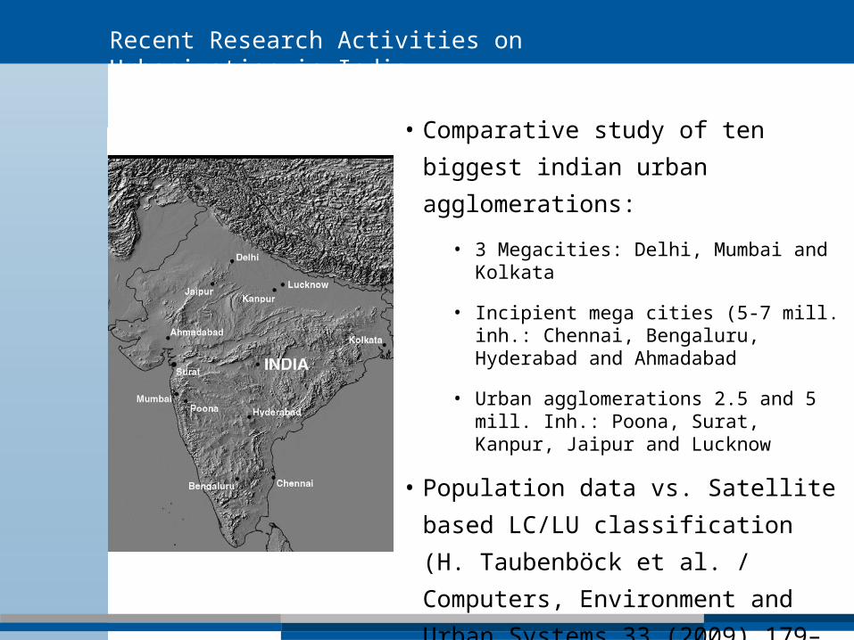
• Comparative study of ten biggest

indian urban agglomerations:

• 3 Megacities: Delhi, Mumbai and Kolkata

• Incipient mega cities (5-7 mill. inh.: Chennai, Bengaluru, Hyderabad and Ahmadabad

• Urban agglomerations 2.5 and 5 mill. Inh.: Poona, Surat, Kanpur, Jaipur and Lucknow

• Population data vs. Satellite based

LC/LU classification (H. Taubenböck

et al. / Computers, Environment

and Urban Systems 33 (2009) 179–

188

Recent Research Activities on Urbanization in India

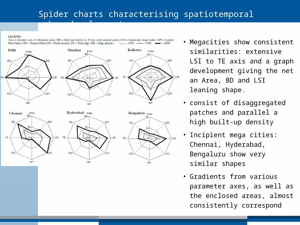
• Megacities show consistent

similarities: extensive LSI to TE

axis and a graph development

giving the net an Area, BD and LSI

leaning shape.

• consist of disaggregated patches

and parallel a high built-up density

• Incipient mega cities: Chennai,

Hyderabad, Bengaluru show very

similar shapes

• Gradients from various parameter

axes, as well as the enclosed

areas, almost consistently

correspond

Spider charts characterising spatiotemporal urban development

Conclusions and Outlook

Remote Sensing and Landscape Metrics widely used during the last decade for evaluating spatio-temporal dynamics in urban regions

Need to standardize/harmonize methods for a real evaluation, especially for inter-urban comparisons, LU/LC budgets and prognosis

How can we integrate case studies into a common and widely accepted framework?

Physical expansion of Hyderabad

Thanks for your attention !

- Degree of spatial concentration and dispersion exhibited by a geographical variable in a specified area

- For all 35 wards and also for four fringe zones i.e. SE, NE, NW and SW

- Results: urban sprawl has occurred in all the wards of twin city but not at the same rate.

- Sprawl has been expected more in the fringe wards but the wards, which are in the city centre, have also experienced development i.e. vertical expansion - some open/vacant lands are now occupied with high rising buildings.

Shannon Entropy value Calculation

36

Urban growth of Hanoi: 2000 (yellow), 2002 (orange), 2011 (red)

Comparison of Spatial Metrics across Regions (Huang et al., 2010)

Correlations between spatial variables (Huang et al., 2010)