1 FundamentalTheoryofResonantMEMSDevices - Wiley … · theory of mechanical vibrations. ... These more advanced aspects of MEMS ... correspond to systems whose free-vibration response

3

1Fundamental Theory of Resonant MEMS DevicesStephen M. Heinrich and Isabelle Dufour

1.1Introduction

Resonators based on MEMS (micro-electromechanical systems) and NEMS(nano-electromechanical systems) span a broad spectrum of important currentapplications, including detection of chemical [1–7] and biological substances[2–4, 6–10], measurement of rheological properties of fluids [11–14], andenergy harvesting [15–17], to name only a few. While the devices that performthese diverse functions span an equally broad range in geometric layout, materialproperties, circuitry, fabrication techniques, packaging, and so on, they all haveone aspect in common: the phenomenon of “resonance” forms the basis oftheir operating principle. More specifically, they usually perform their desiredfunctions by monitoring how interactions with the environment (with various“measurands”) influence the resonant behavior (e.g., the resonant frequency)of the device. Conversely, how effectively the device performs its function willdepend to a large degree on the underlying resonant characteristics of the device(e.g., its quality factor, which determines the resonant peak “sharpness” on a plotof response vs driving frequency). Since all such devices rely on resonant vibra-tions to accomplish one or more tasks effectively, a firm understanding of thishighly interdisciplinary field requires that one be familiar with the fundamentaltheory of mechanical vibrations. To facilitate such familiarity is therefore theprimary goal of this initial chapter.In the sections that follow, an attempt will be made to achieve several specific

objectives. In Section 1.2, a glossary of the major notation and terminology of thechapter will be presented, followed by a summary of the theory of single-degree-of-freedom (SDOF) damped oscillators in Section 1.3 for the cases of free vibra-tion and forced harmonic vibration.This summary, which also includes definitionsof the resonator’s quality factor Q, methods for estimating its value experimen-tally, and a brief discussion of how multiple dissipation sources contribute to Q,is intended to familiarize the reader with the fundamental concepts associatedwith mechanical resonant phenomena. The SDOF section lays the groundworkfor the understanding of multiple-degree-of-freedom (MDOF) dynamic system

Resonant MEMS–Fundamentals, Implementation and Application, First Edition.Edited by Oliver Brand, Isabelle Dufour, Stephen M. Heinrich and Fabien Josse.© 2015 Wiley-VCH Verlag GmbH & Co. KGaA. Published 2015 by Wiley-VCH Verlag GmbH & Co. KGaA.

4 1 Fundamental Theory of Resonant MEMS Devices

behavior, which is the focus of Section 1.4. The mechanical behavior of such sys-tems is introduced by means of two simple, yet highly relevant, examples for acantilever beam, including its free-vibration response and its response due to asinusoidal end force. The solutions presented for the cantilever will be based on a“continuous-systems” (distributed-parameters) modeling approach and will serveas a vehicle for (i) introducing the key concepts of natural/resonant frequenciesand mode shapes for MDOF systems and (ii) showing how the resonant responseof such systems may often be interpreted and approximated as that associatedwith an SDOF system. Section 1.5 furnishes a list of potentially useful natural fre-quency formulas for some of the more common geometries and vibration modesused in resonant MEMS/NEMS applications, while the chapter concludes with abrief summary (Section 1.6).

1.2Nomenclature

A summary of the primary notation and terminology used in this chapter is givenbelow. Note that all of the “𝜔” frequency quantities indicated below are “circular”or “angular” frequencies in that all have units of radians per second. Any of thesefrequencies may be converted to their corresponding frequencies, denoted by “f ,”having units of cycles per second, or hertz, through the relationship f = 𝜔∕2𝜋.

FRF = frequency response function= a plot of a particular response quantity (e.g.,displacement amplitude at a point) vs the actuation frequency when the resonator isexcited by a sinusoidal force;

𝜔 = actuation (exciting) frequency;𝜆 = dimensionless actuation frequency;𝜔0 = undamped natural frequency of an SDOF system (referred to as simply “natural

frequency” by some authors);𝜔d = damped natural frequency of an SDOF system;𝜔res = resonant frequency= the exciting frequency that results in a resonant state, defined

as a vibrational state corresponding to a relative maximum (resonant peak) on theFRF for displacement amplitude; note that some authors define the resonantfrequency as being identical to the undamped natural frequency, not as the excitingfrequency causing peak displacement response; for small damping levels, thedifference in the two values is insignificant;

𝜔n = undamped natural frequency of nth mode of an MDOF system (n= 1, 2, … );𝜆n = dimensionless undamped natural frequency parameter of nth mode of an MDOF

system (n= 1, 2, … );r = frequency ratio, that is, ratio of exciting frequency to undamped natural frequency;𝜁 = damping ratio;Q = quality factor;𝜑n(𝜉) = nth mode shape of a cantilever beam, where the mode shapes represent the set of

possible constant-shape free vibrations, (n= 1, 2, … );

1.3 Single-Degree-of-Freedom (SDOF) Systems 5

𝜓(𝜉) = vibrational shape of a cantilever beam when excited by a harmonic tip force;D = dynamic magnification factor for an SDOF system= ratio of dynamic displacement

amplitude to quasi-static (zero-frequency) value;𝜃 = lag angle by which the steady-state displacement of an SDOF system trails the

applied harmonic force;Dtip = dynamic magnification factor for harmonically loaded cantilever tip= ratio of

dynamic displacement amplitude at beam tip to quasi-static (zero-frequency) value;𝜃tip = lag angle by which the steady-state displacement at the tip of a cantilever trails the

applied harmonic tip force.

The quantities listed above will be examined and discussed in greater detail inthe sections that follow.

1.3Single-Degree-of-Freedom (SDOF) Systems

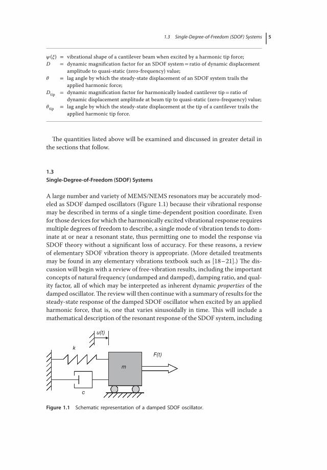
A large number and variety of MEMS/NEMS resonators may be accurately mod-eled as SDOF damped oscillators (Figure 1.1) because their vibrational responsemay be described in terms of a single time-dependent position coordinate. Evenfor those devices for which the harmonically excited vibrational response requiresmultiple degrees of freedom to describe, a single mode of vibration tends to dom-inate at or near a resonant state, thus permitting one to model the response viaSDOF theory without a significant loss of accuracy. For these reasons, a reviewof elementary SDOF vibration theory is appropriate. (More detailed treatmentsmay be found in any elementary vibrations textbook such as [18–21].) The dis-cussion will begin with a review of free-vibration results, including the importantconcepts of natural frequency (undamped and damped), damping ratio, and qual-ity factor, all of which may be interpreted as inherent dynamic properties of thedamped oscillator.The reviewwill then continue with a summary of results for thesteady-state response of the damped SDOF oscillator when excited by an appliedharmonic force, that is, one that varies sinusoidally in time. This will include amathematical description of the resonant response of the SDOF system, including

m

c

k

u(t)

F(t)

Figure 1.1 Schematic representation of a damped SDOF oscillator.


an alternative definition of the quality factor and a resonance-based experimentalmethod (bandwidth method) for measuring Q.In the summary that follows, several assumptions are implicit:

• energy dissipation is due to a viscous damping mechanism (damping force isproportional to velocity);

• the effective mass (m), effective damping coefficient (c), and the effective stiff-ness (k) of the system are constant, that is, they do not depend on time or onthe frequency of oscillation;

• the system is linear, which necessitates that the physical system being modeledas an SDOF oscillator involves linear elastic and linear dissipative forces (thespring and dashpot in Figure 1.1 exhibit material linearity) and small deforma-tions (no geometric nonlinearities).

In certain cases of practical interest, not all damping mechanisms will be ofthe viscous variety, nor will resonators always respond linearly or with frequency-independent properties [19, 21]. Nevertheless, an understanding of simple SDOFresonator behavior based on the above assumptions will provide an importantfoundation for understanding resonator behavior and a logical point of depar-ture for grasping some of the more complex issues that arise when the afore-mentioned assumptions are not met. These more advanced aspects of MEMSresonator response will be treated in many of the chapters that follow.

1.3.1Free Vibration

The assumptions of linear spring and dashpot behavior in the SDOF system ofFigure 1.1 enable one to derive the following equation of motion by performing asimple force balance:

mu(t) + cu(t) + ku(t) = F(t) (1.1)

where m, c, and k represent, respectively, the effective mass, effective dampingcoefficient, and effective stiffness of the system and u(t) is the displacementresponse of the SDOF oscillator. The “dot notation” has been used in Eq. (1.1) torepresent differentiation with respect to time t. The effective externally appliedforce, F(t), is in general related to the excitation force that is applied to theresonator by one of several actuation methods (e.g., electrostatic, electrothermal,piezoelectric). The specific manner in which the effective properties (m, c, k), theeffective applied force F(t), and the displacement u(t) of the idealized system ofFigure 1.1 are related to the physical geometry, material properties, and actuationdetails of a particular device may be derived by the application of first principlesfor a system whose vibrational shape remains constant with time. (See, e.g.,[22–24] for examples involving modeling of MEMS resonators.) For the case offree vibration considered here, the system vibrates in the absence of any externallyapplied force, that is, F(t) ≡ 0, resulting in the homogeneous form of Eq. (1.1):


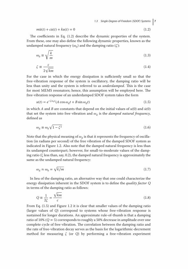
mu(t) + cu(t) + ku(t) = 0 (1.2)

The coefficients in Eq. (1.2) describe the dynamic properties of the system.From these, one may also define the following dynamic properties, known as theundamped natural frequency (𝜔0) and the damping ratio (𝜁 ):

𝜔0 ≡√

km

(1.3)

𝜁 ≡ c2√

km(1.4)

For the case in which the energy dissipation is sufficiently small so that thefree-vibration response of the system is oscillatory, the damping ratio will beless than unity and the system is referred to as underdamped. This is the casefor most MEMS resonators; hence, this assumption will be employed here. Thefree-vibration response of an underdamped SDOF system takes the form

u(t) = e−𝜁𝜔0t(A cos𝜔dt + B sin𝜔dt) (1.5)

in which A and B are constants that depend on the initial values of u(0) and u(0)that set the system into free vibration and 𝜔d is the damped natural frequency,defined as

𝜔d ≡ 𝜔0

√1 − 𝜁2 (1.6)

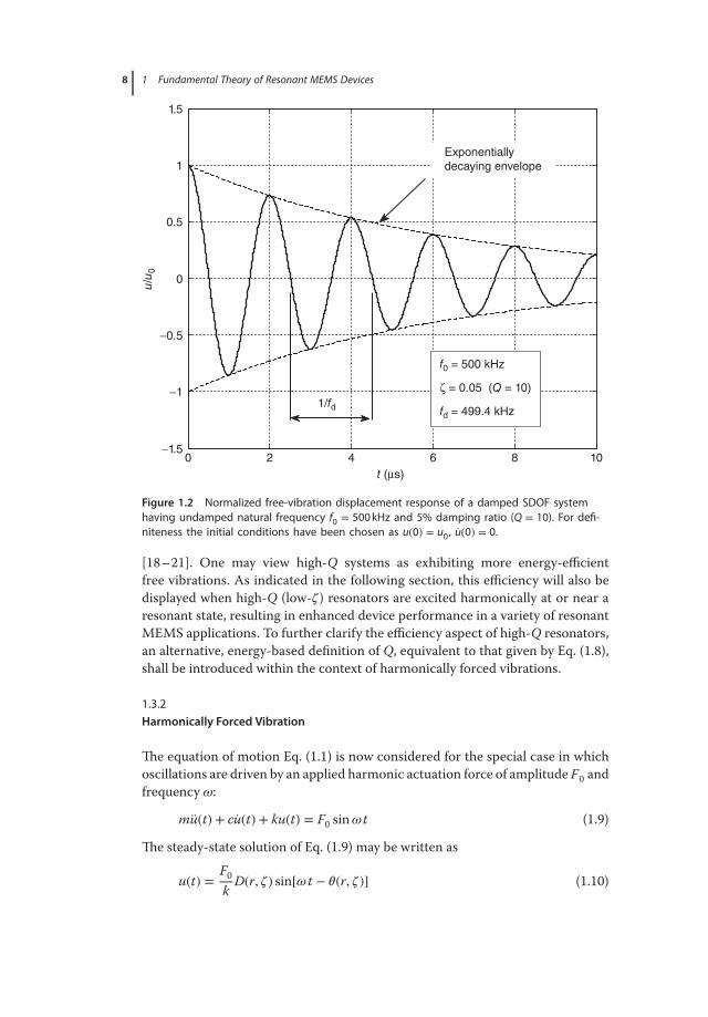
Note that the physical meaning of 𝜔d is that it represents the frequency of oscilla-tion (in radians per second) of the free vibration of the damped SDOF system asindicated in Figure 1.2. Also note that the damped natural frequency is less thanits undamped counterpart; however, for small-to-moderate values of the damp-ing ratio (ζ less than, say, 0.2), the damped natural frequency is approximately thesame as the undamped natural frequency:

𝜔d ≈ 𝜔0 =√

k∕m (1.7)

In lieu of the damping ratio, an alternative way that one could characterize theenergy dissipation inherent in the SDOF system is to define the quality factor Qin terms of the damping ratio as follows:

Q ≡ 12𝜁

=√

kmc

(1.8)

From Eq. (1.5) and Figure 1.2 it is clear that smaller values of the damping ratio(larger values of Q) correspond to systems whose free-vibration response issustained for longer durations. An approximate rule-of-thumb is that a dampingratio of 10% (Q = 5) corresponds to roughly a 50% decrease in amplitude over onecomplete cycle of free vibration. The correlation between the damping ratio andthe rate of free-vibration decay serves as the basis for the logarithmic-decrementmethod for measuring 𝜁 (or Q) by performing a free-vibration experiment


0 2 4 6 8 10−1.5

−1

−0.5

0

0.5

1

1.5

t (μs)

u/u 0

Exponentiallydecaying envelope

1/fd

f0 = 500 kHz

ζ = 0.05 (Q = 10) fd = 499.4 kHz

Figure 1.2 Normalized free-vibration displacement response of a damped SDOF systemhaving undamped natural frequency f0 = 500 kHz and 5% damping ratio (Q = 10). For defi-niteness the initial conditions have been chosen as u(0) = u0, u(0) = 0.

[18–21]. One may view high-Q systems as exhibiting more energy-efficientfree vibrations. As indicated in the following section, this efficiency will also bedisplayed when high-Q (low-𝜁 ) resonators are excited harmonically at or near aresonant state, resulting in enhanced device performance in a variety of resonantMEMS applications. To further clarify the efficiency aspect of high-Q resonators,an alternative, energy-based definition of Q, equivalent to that given by Eq. (1.8),shall be introduced within the context of harmonically forced vibrations.

1.3.2Harmonically Forced Vibration

The equation of motion Eq. (1.1) is now considered for the special case in whichoscillations are driven by an applied harmonic actuation force of amplitude F0 andfrequency 𝜔:

mu(t) + cu(t) + ku(t) = F0 sin𝜔 t (1.9)

The steady-state solution of Eq. (1.9) may be written as

u(t) =F0k

D(r, 𝜁) sin[𝜔 t − 𝜃(r, 𝜁)] (1.10)


where

D(r, 𝜁) ≡ 1√(1 − r2)2 + (2𝜁r)2

(1.11)

𝜃(r, 𝜁) ≡ arctan(

2𝜁r1 − r2

)∈ [0, 𝜋] (1.12)

r ≡ 𝜔

𝜔0(1.13)

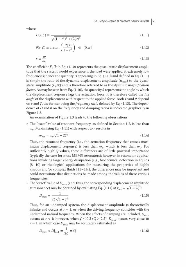
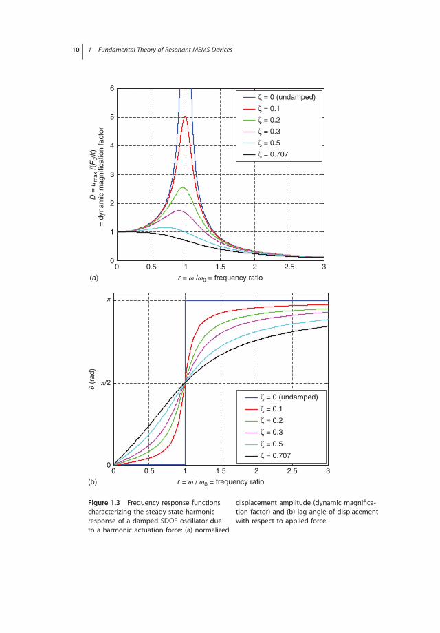
The coefficient F0/k in Eq. (1.10) represents the quasi-static displacement ampli-tude that the system would experience if the load were applied at extremely lowfrequencies; hence the quantity D appearing in Eq. (1.10) and defined in Eq. (1.11)is simply the ratio of the dynamic displacement amplitude (umax) to the quasi-static amplitude (F0/k) and is therefore referred to as the dynamic magnificationfactor. Asmay be seen fromEq. (1.10), the quantity 𝜃 represents the angle bywhichthe displacement response lags the actuation force; it is therefore called the lagangle of the displacement with respect to the applied force. Both D and 𝜃 dependon r and 𝜁 , the former being the frequency ratio defined by Eq. (1.13). The depen-dence of D and 𝜃 on the frequency and damping ratios is indicated graphically inFigure 1.3.An examination of Figure 1.3 leads to the following observations:

• The “exact” value of resonant frequency, as defined in Section 1.2, is less than𝜔0. Maximizing Eq. (1.11) with respect to r results in

𝜔res = 𝜔0

√1 − 2𝜁2 (1.14)

Thus, the resonant frequency (i.e., the actuation frequency that causes max-imum displacement response) is less than 𝜔d, which is less than 𝜔0. Forsufficiently high Q values, these differences are of little practical importance(typically the case for most MEMS resonators); however, in resonator applica-tions involving larger energy dissipation (e.g., biochemical detection in liquids[8–10] or rheological applications for measuring the properties of highlyviscous and/or complex fluids [11–14]), the differences may be important andcould necessitate that distinctions be made among the values of these variousfrequencies.

• The “exact” value of Dmax (and, thus, the corresponding displacement amplitudeat resonance) may be obtained by evaluating Eq. (1.11) at rres =

√1 − 2𝜁2:

Dmax =1

2𝜁√1 − 𝜁2

(1.15)

Thus, for an undamped system, the displacement amplitude is theoreticallyinfinite and occurs at r = 1, or when the driving frequency coincides with theundamped natural frequency. When the effects of damping are included, Dmaxoccurs at r < 1; however, when 𝜁 ≤ 0.2 (Q ≥ 2.5), Dmax occurs very close tor = 1, in which case Dmax may be accurately estimated as

Dmax ≈ D|r=1 =12𝜁

= Q (1.16)


(a)

(b)

0 0.5 1 1.5 2 2.5 30

1

2

3

4

5

6

r = ω /ω0 = frequency ratio

D =

um

ax /(

F0/

k)=

dyn

amic

mag

nific

atio

n fa

ctor

ζ = 0 (undamped)

ζ = 0.1

ζ = 0.2

ζ = 0.3

ζ = 0.5

ζ = 0.707

0 0.5 1 1.5 2 2.5 3

r = ω / ω0 = frequency ratio

θ (r

ad)

ζ = 0 (undamped)

ζ = 0.1

ζ = 0.2

ζ = 0.3

ζ = 0.5

ζ = 0.7070

π/2

π

Figure 1.3 Frequency response functionscharacterizing the steady-state harmonicresponse of a damped SDOF oscillator dueto a harmonic actuation force: (a) normalized

displacement amplitude (dynamic magnifica-tion factor) and (b) lag angle of displacementwith respect to applied force.


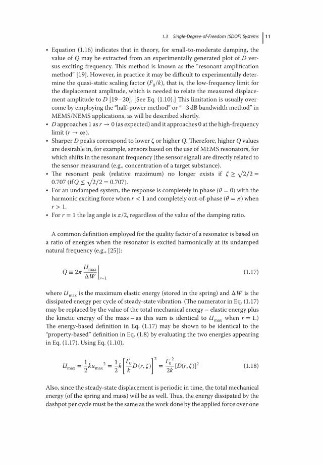
• Equation (1.16) indicates that in theory, for small-to-moderate damping, thevalue of Q may be extracted from an experimentally generated plot of D ver-sus exciting frequency. This method is known as the “resonant amplificationmethod” [19]. However, in practice it may be difficult to experimentally deter-mine the quasi-static scaling factor (F0/k), that is, the low-frequency limit forthe displacement amplitude, which is needed to relate the measured displace-ment amplitude to D [19–20]. [See Eq. (1.10).] This limitation is usually over-come by employing the “half-power method” or “−3 dB bandwidth method” inMEMS/NEMS applications, as will be described shortly.

• D approaches 1 as r → 0 (as expected) and it approaches 0 at the high-frequencylimit (r → ∞).

• Sharper D peaks correspond to lower ζ or higher Q. Therefore, higher Q valuesare desirable in, for example, sensors based on the use of MEMS resonators, forwhich shifts in the resonant frequency (the sensor signal) are directly related tothe sensor measurand (e.g., concentration of a target substance).

• The resonant peak (relative maximum) no longer exists if 𝜁 ≥ √2∕2 =

0.707 (ifQ ≤ √2∕2 = 0.707).

• For an undamped system, the response is completely in phase (𝜃 = 0) with theharmonic exciting force when r < 1 and completely out-of-phase (𝜃 = 𝜋) whenr > 1.

• For r = 1 the lag angle is 𝜋/2, regardless of the value of the damping ratio.

A common definition employed for the quality factor of a resonator is based ona ratio of energies when the resonator is excited harmonically at its undampednatural frequency (e.g., [25]):

Q ≡ 2𝜋UmaxΔW

||||r=1(1.17)

where Umax is the maximum elastic energy (stored in the spring) and ΔW is thedissipated energy per cycle of steady-state vibration. (The numerator in Eq. (1.17)may be replaced by the value of the total mechanical energy – elastic energy plusthe kinetic energy of the mass – as this sum is identical to Umax when r = 1.)The energy-based definition in Eq. (1.17) may be shown to be identical to the“property-based” definition in Eq. (1.8) by evaluating the two energies appearingin Eq. (1.17). Using Eq. (1.10),

Umax =12

kumax2 = 1

2k[F0

kD (r, 𝜁)

]2=

F02

2k[D(r, 𝜁)]2 (1.18)

Also, since the steady-state displacement is periodic in time, the total mechanicalenergy (of the spring and mass) will be as well. Thus, the energy dissipated by thedashpot per cyclemust be the same as the work done by the applied force over one


cycle. Utilizing Eqs. (1.10) and (1.12), the dissipated energy is obtained as follows:

ΔW =∫1 cycleF(t)du = ∫

2𝜋∕𝜔

0F(t)u(t)dt

=∫2𝜋∕𝜔

0F0 sin𝜔t

[F0k

D𝜔 cos (𝜔t − 𝜃)]dt

= … =2𝜋𝜁rF0

2[D(r, 𝜁)]2

k(1.19)

Substituting Eqs. (1.18) and (1.19) into Eq. (1.17) yields

Q ≡ 2𝜋UmaxΔW

||||r=1= 1

2𝜁r||||r=1

= 12𝜁

=√

kmc

(1.20)

that is, the energy-based definition of Q (Eq. (1.17)) is equivalent to the definitiongiven by Eq. (1.8).A common experimental method used to measure Q in MEMS/NEMS res-

onators (and in other resonating structures) is the bandwidth method, also knownas the −3 dB bandwidth method or the half-power method [2, 20]. This methodis based on taking advantage of the Q-dependence of the shape of the FRF for theresponse amplitude in the vicinity of the resonant peak (Figure 1.3a).The FRF maybe for the displacement amplitude or any output signal “R” that is proportional tothe displacement amplitude (e.g., electrical voltage). Having experimentally deter-mined the shape of the resonant peak, the value of Q may be estimated by theformula

Q ≈𝜔resΔ𝜔

=fresΔf

(1.21)

in which 𝜔res is the resonant frequency (defined by the peak response value Rmaxof the FRF), Δ𝜔 ≡ 𝜔2–𝜔1 is the frequency bandwidth and 𝜔1 and 𝜔2 are the fre-quencies corresponding to a response value of Rmax/

√2. Analogous definitions

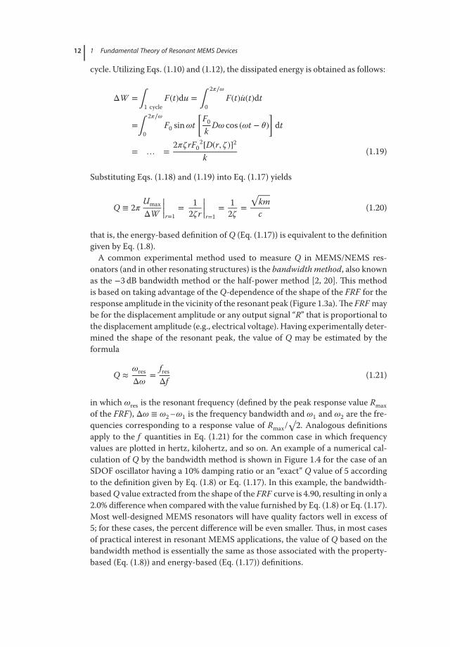
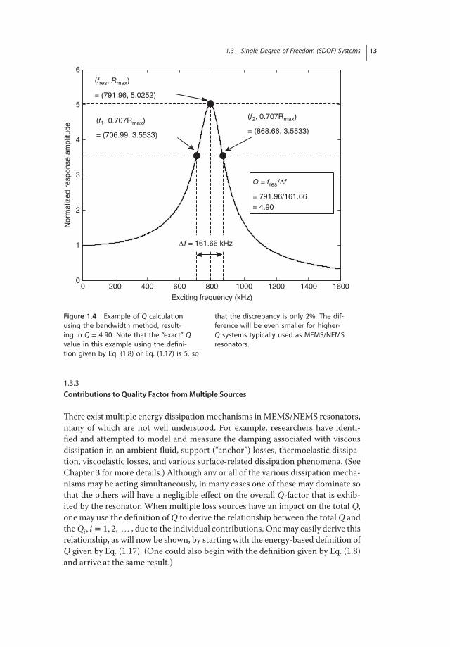
apply to the f quantities in Eq. (1.21) for the common case in which frequencyvalues are plotted in hertz, kilohertz, and so on. An example of a numerical cal-culation of Q by the bandwidth method is shown in Figure 1.4 for the case of anSDOF oscillator having a 10% damping ratio or an “exact” Q value of 5 accordingto the definition given by Eq. (1.8) or Eq. (1.17). In this example, the bandwidth-based Q value extracted from the shape of the FRF curve is 4.90, resulting in only a2.0% difference when compared with the value furnished by Eq. (1.8) or Eq. (1.17).Most well-designed MEMS resonators will have quality factors well in excess of5; for these cases, the percent difference will be even smaller. Thus, in most casesof practical interest in resonant MEMS applications, the value of Q based on thebandwidth method is essentially the same as those associated with the property-based (Eq. (1.8)) and energy-based (Eq. (1.17)) definitions.


0 200 400 600 800 1000 1200 1400 16000

1

2

3

4

5

6N

orm

aliz

ed r

espo

nse

ampl

itude

Exciting frequency (kHz)

(fres, Rmax)

= (791.96, 5.0252)

(f2, 0.707Rmax)

= (868.66, 3.5533)(f1, 0.707Rmax)

= (706.99, 3.5533)

Q = fres/Δf

= 791.96/161.66 = 4.90

Δ f = 161.66 kHz

Figure 1.4 Example of Q calculationusing the bandwidth method, result-ing in Q = 4.90. Note that the “exact” Qvalue in this example using the defini-tion given by Eq. (1.8) or Eq. (1.17) is 5, so

that the discrepancy is only 2%. The dif-ference will be even smaller for higher-Q systems typically used as MEMS/NEMSresonators.

1.3.3Contributions to Quality Factor fromMultiple Sources

There exist multiple energy dissipationmechanisms inMEMS/NEMS resonators,many of which are not well understood. For example, researchers have identi-fied and attempted to model and measure the damping associated with viscousdissipation in an ambient fluid, support (“anchor”) losses, thermoelastic dissipa-tion, viscoelastic losses, and various surface-related dissipation phenomena. (SeeChapter 3 for more details.) Although any or all of the various dissipation mecha-nisms may be acting simultaneously, in many cases one of these may dominate sothat the others will have a negligible effect on the overall Q-factor that is exhib-ited by the resonator. When multiple loss sources have an impact on the total Q,one may use the definition of Q to derive the relationship between the total Q andthe Qi, i = 1, 2, … , due to the individual contributions. Onemay easily derive thisrelationship, as will now be shown, by starting with the energy-based definition ofQ given by Eq. (1.17). (One could also begin with the definition given by Eq. (1.8)and arrive at the same result.)


Assuming that the various sources of energy dissipation in the resonator areindependent, Eq. (1.17) may be written as

Q ≡ 2𝜋Umax

ΔW1 + ΔW2 + …||||r=1

(1.22)

in which ΔWi, i = 1, 2, … , represents the dissipated energy per cycle due to theindividual damping mechanisms. Inverting Eq. (1.22) gives

1Q

= 12𝜋

ΔW1 + ΔW2 + …Umax

|||||r=1= 1

Q1+ 1

Q2+ … (1.23)

or

Q = 11

Q1+ 1

Q2+ …

(1.24)

which is the desired result relating the total Q of the system to the individual Qivalues. Clearly, it follows from Eq. (1.24) that

Q ≈ Qmin (1.25)

for the case in which the smallest of the Qi, denoted by Qmin, is much smallerthan the Qi corresponding to all other damping sources. This is a situation thatmay occur, for example, for in-vacuum or low-pressure gas applications in whichsupport losses could dominate or for liquid-phase applications in which viscousdissipation in the liquid tends to be themajor dampingmechanism inmany cases.

1.4Continuous Systems Modeling: Microcantilever Beam Example

In Section 1.3, some important fundamentals of both free vibration and harmoni-cally forced vibration of an idealized SDOF oscillator were summarized. However,in reality all dynamic systems have the potential to respond in a manner thatrequires a MDOF description in order to capture multiple “modes” of vibrationthat may occur, including the possible interaction of these modes during a free orforced vibration. Two approaches exist for modeling the MDOF response of suchsystems: a discrete-coordinate description and a continuous modeling approach.In the discrete-coordinate approach, the systemproperties are often idealized in

such a manner that the inertial properties and the stiffness properties are uncou-pled; in other words, those portions that have mass are assumed rigid, while thoseparts having flexibility are assumed to be massless. As a result, the system posi-tion at any timemay be expressed in terms of the displacements (and/or rotations)of a finite number of discrete locations in the system. In fact, modeling usingthe finite element method (FEM) falls into this category as it is based on a sys-tematic approach for lumping mass and stiffness characteristics of the system atthe “nodes” of the finite element model. (This modeling approach is discussed inmore detail in Chapter 5.) The mathematical model resulting from the discrete

1.4 Continuous Systems Modeling: Microcantilever Beam Example 15

approach is a set of ordinary differential equations (ODEs) in time, usually writtenin a matrix form.The continuous modeling approach aims to maintain the distributed nature

of the system’s mass and stiffness characteristics and does so by representingthe vibrational response in terms of continuous variables – for example, beamdeflection as a function of a continuous coordinate x ranging from 0 to L (beamlength) – in lieu of a discrete representation. This type of model thereforecomprises an infinite number of degrees of freedom, yielding a mathematicaldescription involving one or more partial differential equations (PDEs).The aimof the present section is to provide a concise overview of the continuous

systems modeling approach by examining the vibration of a cantilever beam.Themotivation for this particular focus is threefold:

1) While obtaining solutions of the PDE(s) of the continuousmodeling approachtends to be, in general, more difficult than solving the ODEs of the discretemethod, in the case of manyMEMS resonators, the geometries tend to be rel-atively simple and therefore amenable to the continuous modeling approach.

2) Micro- and nanocantilevers are quite prominent in a variety of resonantMEMS applications due to their ease of fabrication, portability, and versatil-ity [4, 7, 10]. Hence, the example furnished by a cantilever beam will yieldspecific results that are highly relevant to many cantilever-based resonantdevices.

3) The simple example of a cantilever serves as an ideal vehicle for presentingthe general modeling approach, terminology, and concepts that are equallyapplicable to cases of other resonator geometries and boundary conditions(BCs) (e.g., doubly clamped “bridge” beams, membrane disks), the details ofwhich may be found elsewhere (e.g., [26] and the references cited therein).

1.4.1Modeling Assumptions

The continuous model for the vibration of a cantilever beam (Figure 1.5) will bebased on the following assumptions:

• The mass and stiffness properties are constant (independent of time and fre-quency);

• The beam is prismatic (the cross section is uniform along the beam length);• The cross section has an axis of symmetry and the beam vibration occurs alongthe direction of this axis;

• The system is linear: the beam is composed of a linear elastic isotropic materialand the beam deformation is small (slopes of the bent beam are much less thanunity);

• The kinematic assumptions of Bernoulli-Euler beam theory apply: crosssections of the beam remain planar during the deformation (no cross-sectionalwarping) and they remain normal to the deformed beam axis (no transverse


F(t)q(, t)

v(, t)

x, = x/L

L

v

m, EI

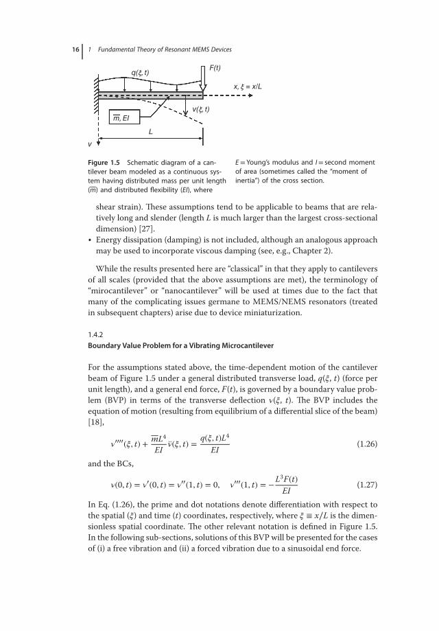
Figure 1.5 Schematic diagram of a can-tilever beam modeled as a continuous sys-tem having distributed mass per unit length(m) and distributed flexibility (EI), where

E = Young’s modulus and I= second momentof area (sometimes called the “moment ofinertia”) of the cross section.

shear strain). These assumptions tend to be applicable to beams that are rela-tively long and slender (length L is much larger than the largest cross-sectionaldimension) [27].

• Energy dissipation (damping) is not included, although an analogous approachmay be used to incorporate viscous damping (see, e.g., Chapter 2).

While the results presented here are “classical” in that they apply to cantileversof all scales (provided that the above assumptions are met), the terminology of“mirocantilever” or “nanocantilever” will be used at times due to the fact thatmany of the complicating issues germane to MEMS/NEMS resonators (treatedin subsequent chapters) arise due to device miniaturization.

1.4.2Boundary Value Problem for a Vibrating Microcantilever

For the assumptions stated above, the time-dependent motion of the cantileverbeam of Figure 1.5 under a general distributed transverse load, q(𝜉, t) (force perunit length), and a general end force, F(t), is governed by a boundary value prob-lem (BVP) in terms of the transverse deflection 𝜈(𝜉, t). The BVP includes theequation of motion (resulting from equilibrium of a differential slice of the beam)[18],

𝜈′′′′(𝜉, t) + mL4

EI��(𝜉, t) =

q(𝜉, t)L4

EI(1.26)

and the BCs,

𝜈(0, t) = 𝜈′(0, t) = 𝜈′′(1, t) = 0, 𝜈′′′(1, t) = −L3F(t)EI

(1.27)

In Eq. (1.26), the prime and dot notations denote differentiation with respect tothe spatial (𝜉) and time (t) coordinates, respectively, where 𝜉 ≡ x∕L is the dimen-sionless spatial coordinate. The other relevant notation is defined in Figure 1.5.In the following sub-sections, solutions of this BVP will be presented for the casesof (i) a free vibration and (ii) a forced vibration due to a sinusoidal end force.


1.4.3Free-Vibration Response of Microcantilever

The BVP reduces to its homogeneous form in the case of a free vibration:

𝜈′′′′(𝜉, t) + mL4

EI��(𝜉, t) = 0 (1.28)

𝜈(0, t) = 𝜈′(0, t) = 𝜈′′(1, t) = 𝜈′′′(1, t) = 0 (1.29)

Solutions are assumed to be in the form of “modal vibrations,” that is, free vibra-tions of a constant shape:

𝜈(𝜉, t) = 𝜑n(𝜉)(A cos𝜔nt + B sin𝜔nt), n = 1, 2, … (1.30)

in which 𝜔n is the natural frequency of the nth mode and 𝜑n(𝜉) is the correspond-ing mode shape, both of which have yet to be determined. Placing Eq. (1.30) intoEqs. (1.28) and (1.29) yields the following eigenvalue problem for determiningthe dimensionless natural frequencies (eigenvalues) 𝜆n and the associated modeshapes (eigenfunctions or eigenmodes) 𝜑n(𝜉):

𝜑′′′′n (𝜉) − 𝜆n

4𝜑n(𝜉) = 0,(𝜆n

4 ≡ mL4𝜔n2

EI

)(1.31)

𝜑n(0) = 𝜑′n(0) = 𝜑′′

n (1) = 𝜑′′′n (1) = 0 (1.32)

The general solution of Eq. (1.31) is of the form

𝜑n(𝜉) = A1 cosh 𝜆n𝜉 + A2 cos 𝜆n𝜉 + A3 sinh 𝜆n𝜉 + A4 sin 𝜆n𝜉 (1.33)

which, when placed into Eqs. (1.32), results in a linear algebraic systemof the form

[G(𝜆n)]{A} = {0} (1.34)

for determining the coefficients in Eq. (1.33). Non-trivial solutions for the vector{A} only exist if the 𝜆n-dependent coefficientmatrix is singular, thus requiring thatdet[G(𝜆n)] = 0 or, after simplifying,

1 + cosh 𝜆n cos 𝜆n = 0 (1.35)

Equation (1.35) is referred to as the frequency equation of the cantilever beam. Itsroots, which by convention are numbered in increasing order, are given by (foursignificant figures)

𝜆1 ≡ 1.875, 𝜆2 ≡ 4.694, 𝜆3 ≡ 7.855, 𝜆n ≈ (2n − 1)𝜋2

for n > 3 (1.36)

The corresponding (undamped) natural frequencies of the cantilever are given bythe definition listed with Eq. (1.31), that is,

𝜔n = 𝜆n2√

EImL4

or fn =𝜆n

2

2𝜋

√EI

mL4(1.37)


0 0.2 0.4 0.6 0.8 1−1

−0.8

−0.6

−0.4

−0.2

0

0.2

0.4

0.6

0.8

1

ξ = x/L

ϕ n

n = 1 (λ1 = 1.875)

n = 2 (λ2 = 4.694)

n = 3 (λ3 = 7.855)

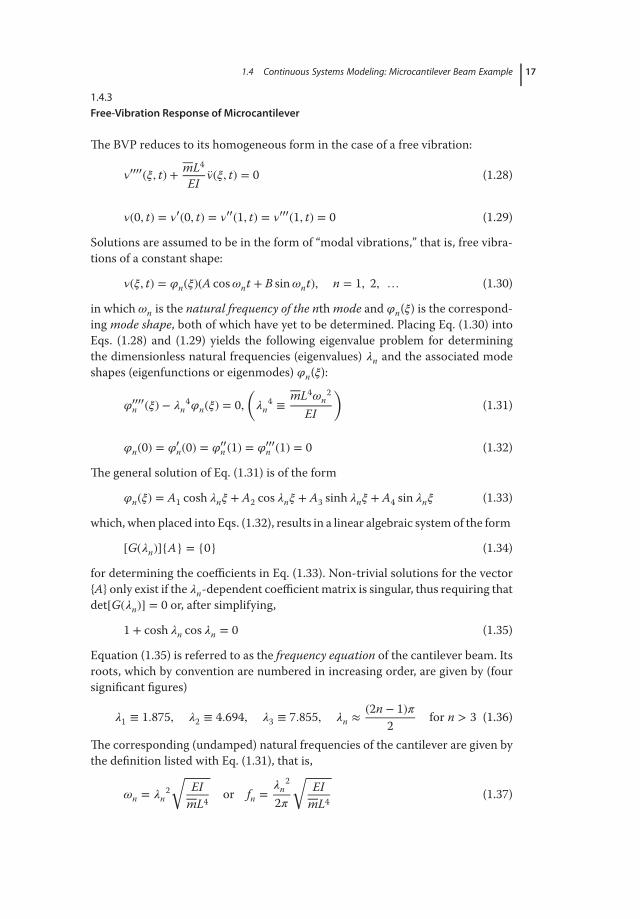
Figure 1.6 First three mode shapes of a cantilever beam. The plots have been normalizedsuch that the tip deflection is (−1)n+1, where n is the mode number.

The mode shapes are determined by placing each eigenvalue listed in Eq. (1.36)into Eq. (1.34), solving Eq. (1.34) for the constants A2, A3, A4 in terms of A1, andsubstituting the result into Eq. (1.33). This yields the individual modes shapes,𝜑n(𝜉), n = 1, 2, … , corresponding to each of the natural frequencies:

𝜑n(𝜉) = A1(n)

[cosh 𝜆n𝜉 − cos 𝜆n𝜉 −

(cosh 𝜆n + cos 𝜆nsinh 𝜆n + sin 𝜆n

)(sinh 𝜆n𝜉 − sin 𝜆n𝜉)

](1.38)

The constant A1(n) for each mode is arbitrary; its value may be chosen to scale the

mode shape in anymanner that is deemed convenient. Plots of the first threemodeshapes for a cantilever beam are shown in Figure 1.6. Each mode shape shownhas one or more locations at which the beam displacement is zero. Such pointsthat experience no movement during a modal vibration are known as vibrationalnodes. In general, the number of vibrational nodes will increase as the mode num-ber n increases. The location of the nodes has important practical implications inresonant MEMS applications in that a designer may minimize the energy lossesassociated with supporting structures by placing the resonator supports at or nearthe vibrational nodes of the resonator. (See Chapters 3 and 5 for more details.)


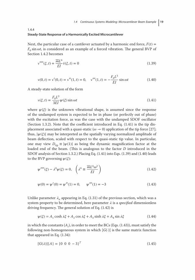
1.4.4Steady-State Response of a Harmonically Excited Microcantilever

Next, the particular case of a cantilever actuated by a harmonic end force, F(t) =F0 sin𝜔t, is considered as an example of a forced vibration. The general BVP ofSection 1.4.2 becomes

𝜈′′′′(𝜉, t) + mL4

EI��(𝜉, t) = 0 (1.39)

𝜈(0, t) = 𝜈′(0, t) = 𝜈′′(1, t) = 0, 𝜈′′′(1, t) = −F0L3

EIsin𝜔t (1.40)

A steady-state solution of the form

𝜈(𝜉, t) =F0L3

3EI𝜓(𝜉) sin𝜔t (1.41)

where 𝜓(𝜉) is the unknown vibrational shape, is assumed since the responseof the undamped system is expected to be in phase (or perfectly out of phase)with the excitation force, as was the case with the undamped SDOF oscillator(Section 1.3.2). Note that the coefficient introduced in Eq. (1.41) is the tip dis-placement associated with a quasi-static (𝜔→ 0) application of the tip force [27];thus, |𝜓(𝜉)| may be interpreted as the spatially varying normalized amplitude ofbeam deflection, scaled with respect to the quasi-static tip value. In particular,one may view Dtip ≡ |𝜓(1)| as being the dynamic magnification factor at theloaded end of the beam. (This is analogous to the factor D introduced in theSDOF analysis of Section 1.3.2.) Placing Eq. (1.41) into Eqs. (1.39) and (1.40) leadsto the BVP governing 𝜓(𝜉):

𝜓 ′′′′(𝜉) − 𝜆4𝜓(𝜉) = 0,(𝜆4 ≡ mL4𝜔2

EI

)(1.42)

𝜓(0) = 𝜓 ′(0) = 𝜓 ′′(1) = 0, 𝜓 ′′′(1) = −3 (1.43)

Unlike parameter 𝜆n appearing in Eq. (1.31) of the previous section, which was asystem property to be determined, here parameter 𝜆 is a specified dimensionlessdriving frequency. The general solution of Eq. (1.42) is

𝜓(𝜉) = A1 cosh 𝜆𝜉 + A2 cos 𝜆𝜉 + A3 sinh 𝜆𝜉 + A4 sin 𝜆𝜉 (1.44)

in which the constants (Ai), in order to meet the BCs (Eqs. (1.43)), must satisfy thefollowing non-homogeneous system in which [G(⋅)] is the same matrix functionthat appeared in Eq. (1.34):

[G(𝜆)]{A} = {0 0 0 − 3}T (1.45)


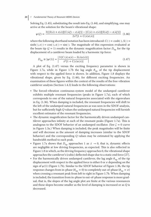
Solving Eq. (1.45), substituting the result into Eq. (1.44), and simplifying, one mayarrive at the solution for the beam’s vibrational shape:

𝜓(𝜉) = 3{[S(𝜆) + s(𝜆)][C(𝜆𝜉) − c(𝜆𝜉)] − [C(𝜆) + c(𝜆)][S(𝜆𝜉) − s(𝜆𝜉)]}2𝜆3[1 + C(𝜆)c(𝜆)]

(1.46)

where the following shorthandnotation has been introduced:C(⋅) = cosh(⋅), S(⋅) =sinh(⋅), c(⋅) = cos(⋅), s(⋅) = sin(⋅). The magnitude of this expression evaluated atthe beam tip (𝜉 = 1) results in the dynamic magnification factor Dtip for the tipdisplacement of a cantilever beam loaded by a harmonic tip force:

Dtip ≡ |𝜓(1)| = ||||3 [C (𝜆) s(𝜆) − S(𝜆)c(𝜆)]𝜆3[1 + C(𝜆)c(𝜆)]

|||| (1.47)

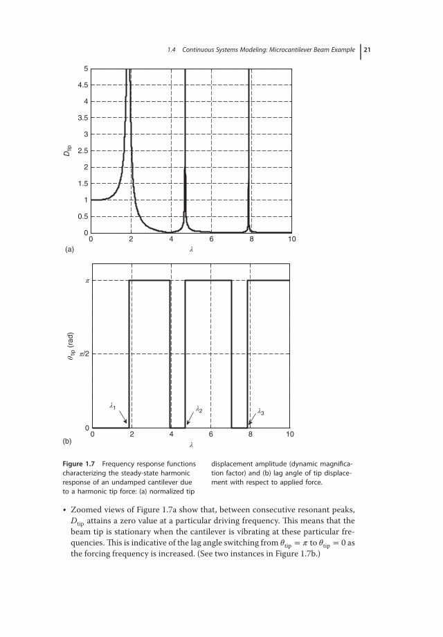
A plot of Eq. (1.47) versus the exciting frequency parameter is shown inFigure 1.7a, while in Figure 1.7b the lag angle 𝜃tip of the tip displacementwith respect to the applied force is shown. In addition, Figure 1.8 displays thevibrational shape, given by Eq. (1.46), for different exciting frequencies. Anexamination of these figures within the context of the results of the free-vibrationcantilever analysis (Section 1.4.3) leads to the following observations:

• The forced-vibration continuous-system model of the undamped cantileverexhibits multiple resonant frequencies (peaks in Figure 1.7a), each of whichcorresponds to one of the natural frequencies associated with the eigenvaluesin Eq. (1.36). When damping is included, the resonant frequencies will shift tothe left of the undamped natural frequencies as was seen in the SDOF analysis,but for sufficiently high Q values the undamped natural frequencies will furnishexcellent estimates of the resonant frequencies.

• The dynamic magnification factor for the harmonically driven undamped can-tilever approaches infinity at each of the resonant peaks (Figure 1.7a). This isanalogous to the SDOF behavior of an undamped oscillator. (See 𝜁 = 0 curvein Figure 1.3a.) When damping is included, the peak magnitudes will be finiteand will decrease as the amount of damping increases (similar to the SDOFbehavior) and the corresponding Q values may be estimated by applying thebandwidth method to each peak.

• Figure 1.7a shows that Dtip approaches 1 as 𝜆 → 0, that is, dynamic effectsare negligible at low driving frequencies, as expected. This is also reflected inFigure 1.8 in which, as the driving frequency approaches 0, the vibrational shapeapproaches the cantilever’s (cubic) deflected shape due to a static end force [27].

• For the harmonically driven undamped cantilever, the lag angle 𝜃tip of the tipdisplacement with respect to the applied force is either 0 or 𝜋 depending on thesign of 𝜓(1) (Figure 1.7b). Similar to the SDOF behavior of Figure 1.3b, the tipresponse changes from in-phase (𝜃tip = 0) to completely out-of-phase (𝜃tip = 𝜋)when crossing a resonant peak from left to right in Figure 1.7b. When dampingis included, the transition from in-phase to out-of-phase response is more grad-ual, that is, the slopes of the lag angle plot are finite at the various resonancesand these slopes become smaller as the level of damping is increased or as Q isdecreased.


(a)

(b)

0 2 4 6 8 100

0.5

1

1.5

2

2.5

3

3.5

4

4.5

5

λ

Dtip

0 2 4 6 8 10λ

θ tip

(ra

d)

π

π/2

0

λ2 λ3λ1

Figure 1.7 Frequency response functionscharacterizing the steady-state harmonicresponse of an undamped cantilever dueto a harmonic tip force: (a) normalized tip

displacement amplitude (dynamic magnifica-tion factor) and (b) lag angle of tip displace-ment with respect to applied force.

• Zoomed views of Figure 1.7a show that, between consecutive resonant peaks,Dtip attains a zero value at a particular driving frequency. This means that thebeam tip is stationary when the cantilever is vibrating at these particular fre-quencies.This is indicative of the lag angle switching from 𝜃tip = 𝜋 to 𝜃tip = 0 asthe forcing frequency is increased. (See two instances in Figure 1.7b.)


0 0.2 0.4 0.6 0.8 1−1.5

−1

−0.5

0

0.5

1

ξ = x/L

Nor

mal

ized

bea

m d

efle

ctio

n

λ = 0 (quasi-static)

λ = 1

λ = λ1 = 1.875

λ = 2.5

λ = 3.5

λ = 4.5

λ = λ2 = 4.694

λ = 5

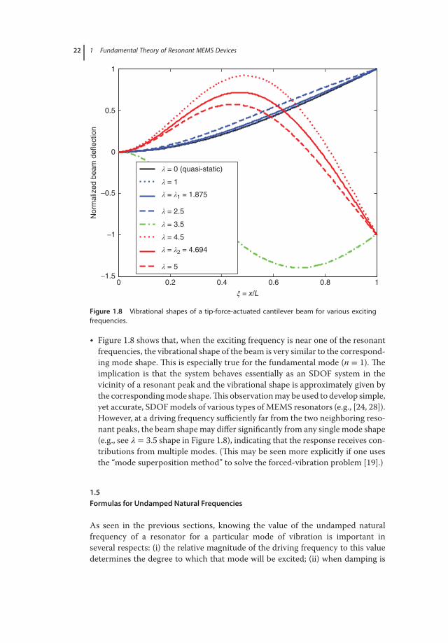
Figure 1.8 Vibrational shapes of a tip-force-actuated cantilever beam for various excitingfrequencies.

• Figure 1.8 shows that, when the exciting frequency is near one of the resonantfrequencies, the vibrational shape of the beam is very similar to the correspond-ing mode shape. This is especially true for the fundamental mode (n = 1). Theimplication is that the system behaves essentially as an SDOF system in thevicinity of a resonant peak and the vibrational shape is approximately given bythe correspondingmode shape.This observationmay be used to develop simple,yet accurate, SDOFmodels of various types ofMEMS resonators (e.g., [24, 28]).However, at a driving frequency sufficiently far from the two neighboring reso-nant peaks, the beam shape may differ significantly from any single mode shape(e.g., see 𝜆 = 3.5 shape in Figure 1.8), indicating that the response receives con-tributions from multiple modes. (This may be seen more explicitly if one usesthe “mode superposition method” to solve the forced-vibration problem [19].)

1.5Formulas for Undamped Natural Frequencies

As seen in the previous sections, knowing the value of the undamped naturalfrequency of a resonator for a particular mode of vibration is important inseveral respects: (i) the relative magnitude of the driving frequency to this valuedetermines the degree to which that mode will be excited; (ii) when damping is

1.5 Formulas for Undamped Natural Frequencies 23

relatively small, the undamped natural frequency furnishes a good estimate ofthe resonant frequency; (iii) the undamped natural frequency yields an upperbound on the resonant frequency when damping and/or the effective mass of anysurrounding fluid is significant; and (iv) in more detailed theoretical pursuits theundamped natural frequency may serve as a convenient reference frequency fornormalizing the system’s actual resonant frequency. All of these reasons providethe motivation in this section to catalog several formulas for determining theundamped natural frequencies for some of the more common device geometriesand vibration modes that are encountered in resonant MEMS applications. Allformulas listed are for circular frequency (units of radians per second) and, asnoted earlier, may be converted to hertz (cycles per second) by dividing by 2𝜋.Within each class of structure type and vibration mode considered, the rangeof the mode number n corresponding to the 𝜔n formula is n = 1, 2, … , where𝜔1 < 𝜔2 < … . Rigid-body (zero-frequency) modes are not considered; thus, inall cases 𝜔1 > 0.For conciseness, the derivations of the formulas presented here are not

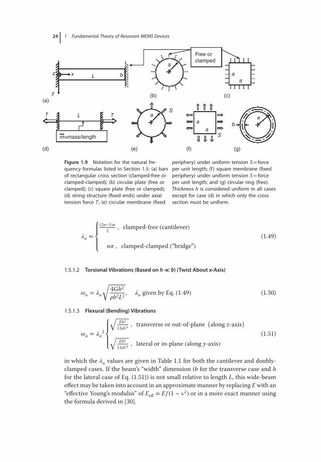
included, but the reader is encouraged to seek out details regarding the originof these formulas as well as the details associated with the corresponding modeshapes. Such details may be found in [26] and in the sources cited therein. Allof the formulas listed are based on the assumptions that the material is linearelastic and isotropic with Young’s modulus E, shear modulus G, and Poisson’sratio 𝜈. Therefore, when applying the results to an anisotropic material, suchas silicon, care should be taken in specifying the equivalent isotropic elasticconstants corresponding to the appropriate direction(s). (See [29] for guidance insuch cases.) Also, each device is assumed to have a uniform mass density 𝜌 (perunit volume), all support conditions are considered “ideal” (perfectly “clamped,”perfectly “free,” etc.), effects of any surrounding fluid are neglected, and, unlessindicated otherwise, all devices are assumed to have a uniform thickness h.Definitions of other parameters appearing in the formulas are given in Figure 1.9.Note that results for “free” (i.e., unsupported) conditions are included, despitethe fact that all MEMS/NEMS resonators involve some type of supportingstructure(s); the justification is that a strategic placement of supports near theresonator’s vibrational nodes will result in the free BCs being approximatelysatisfied and, as stated earlier, minimal energy dissipation via support losses.

1.5.1Simple Deformations (Axial, Bending, Twisting) of 1D Structural Members: Cantileversand Doubly ClampedMembers (“Bridges”)

The relevant device parameters in this section are defined in Figure 1.9a.

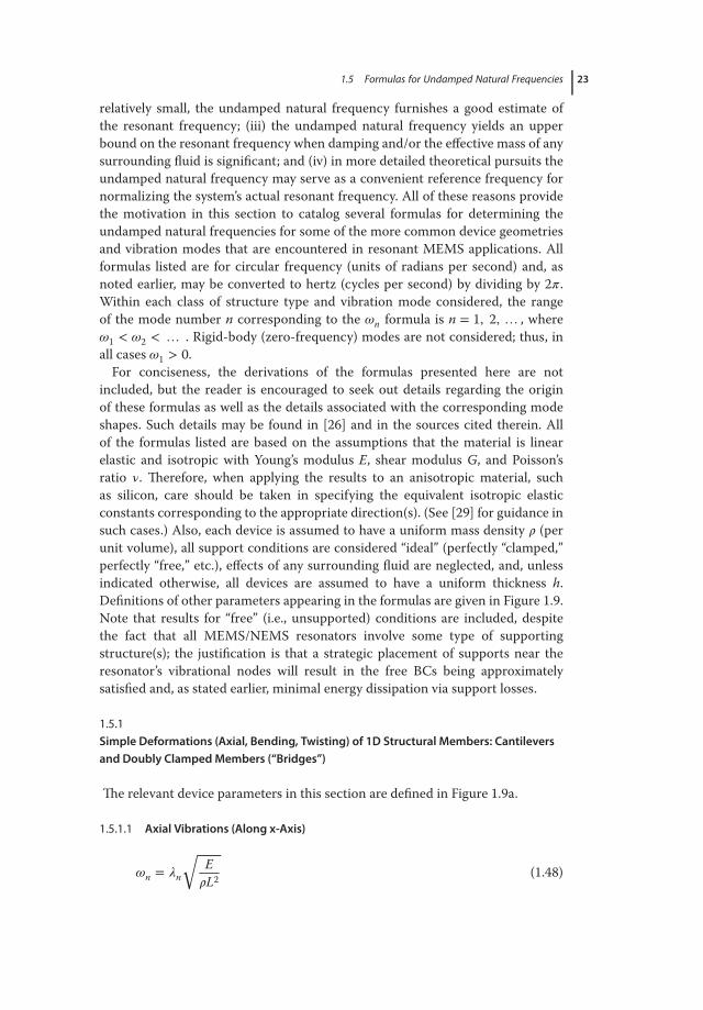
1.5.1.1 Axial Vibrations (Along x-Axis)

𝜔n = 𝜆n

√E𝜌L2 (1.48)


Free orclamped

(a)(b) (c)

(d) (e) (f) (g)

aa

a

a

a

aa

S

S

T T

y

z x L

m=mass/length

b

L

b

Figure 1.9 Notation for the natural fre-quency formulas listed in Section 1.5: (a) barsof rectangular cross section (clamped-free orclamped-clamped); (b) circular plate (free orclamped); (c) square plate (free or clamped);(d) string structure (fixed ends) under axialtension force T ; (e) circular membrane (fixed

periphery) under uniform tension S= forceper unit length; (f ) square membrane (fixedperiphery) under uniform tension S= forceper unit length; and (g) circular ring (free).Thickness h is considered uniform in all casesexcept for case (d) in which only the crosssection must be uniform.

𝜆n =⎧⎪⎨⎪⎩

(2n−1)𝜋2

, clamped-free (cantilever)

n𝜋 , clamped-clamped (“bridge”)(1.49)

1.5.1.2 Torsional Vibrations (Based on h≪ b) (Twist About x-Axis)

𝜔n = 𝜆n

√4Gh2

𝜌b2L2 , 𝜆n given by Eq. (1.49) (1.50)

1.5.1.3 Flexural (Bending) Vibrations

𝜔n = 𝜆n2

⎧⎪⎨⎪⎩

√Eh2

12𝜌L4 , transverse or out-of-plane(along z-axis

)√

Eb2

12𝜌L4 , lateral or in-plane (along y-axis)(1.51)

in which the 𝜆n values are given in Table 1.1 for both the cantilever and doubly-clamped cases. If the beam’s “width” dimension (b for the transverse case and hfor the lateral case of Eq. (1.51)) is not small relative to length L, this wide-beameffect may be taken into account in an approximatemanner by replacing E with an“effective Young’s modulus” of Eeff = E∕(1 − 𝜈2) or in a more exact manner usingthe formula derived in [30].

1.5 Formulas for Undamped Natural Frequencies 25

Table 1.1 Dimensionless coefficients for calculating the natural frequencies for the flexuralmodes of a beam using Eq. (1.51).

Clamped-free(cantilever)

Clamped-clamped(“bridge”)

𝜆1 1.875 4.730𝜆2 4.694 7.853𝜆3 7.855 10.996𝜆n, n > 3 (2n − 1)𝜋∕2 (2n + 1)𝜋∕2

Table 1.2 Dimensionless coefficients for calculating the natural frequencies for the trans-verse deflection of circular and square plates under fully free and fully clamped conditionsusing Eq. (1.52).

Circular plate Square plateFreely supportedalong periphery(𝝂= 0.33)

Clamped alongperiphery(arbitrary 𝛎)

Freely supportedalong periphery(𝝂= 0.3)

Clamped alongperiphery(arbitrary 𝛎)

𝜆12 5.253 10.22 13.49 35.99

𝜆22 9.084 21.26 19.79 73.41

𝜆32 12.23 34.88 24.43 108.3

𝜆42 20.52 39.77 35.02 131.6

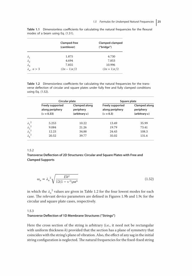
1.5.2Transverse Deflection of 2D Structures: Circular and Square Plates with Free andClamped Supports

𝜔n = 𝜆n2√

Eh2

12(1 − 𝜈 2)𝜌a4 (1.52)

in which the 𝜆n2 values are given in Table 1.2 for the four lowest modes for each

case. The relevant device parameters are defined in Figures 1.9b and 1.9c for thecircular and square plate cases, respectively.

1.5.3Transverse Deflection of 1DMembrane Structures (“Strings”)

Here the cross section of the string is arbitrary (i.e., it need not be rectangularwith uniform thickness h) provided that the section has a plane of symmetry thatcoincideswith the string’s plane of vibration. Also, the effect of any sag in the initialstring configuration is neglected.The natural frequencies for the fixed-fixed string


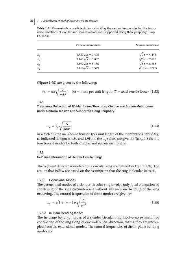
Table 1.3 Dimensionless coefficients for calculating the natural frequencies for the trans-verse vibrations of circular and square membranes supported along their periphery usingEq. (1.54).

Circular membrane Square membrane

𝜆1 1.357√𝜋 = 2.405

√2𝜋 = 4.443

𝜆2 2.162√𝜋 = 3.832

√5𝜋 = 7.025

𝜆3 2.897√𝜋 = 5.135

√8𝜋 = 8.886

𝜆4 3.114√𝜋 = 5.519

√10𝜋 = 9.935

(Figure 1.9d) are given by the following:

𝜔n = n𝜋√

TmL2

, (m = mass per unit length, T = axial tensile force) (1.53)

1.5.4Transverse Deflection of 2DMembrane Structures: Circular and Square Membranesunder Uniform Tension and Supported along Periphery

𝜔n = 𝜆n

√S

𝜌ha2 (1.54)

in which S is the membrane tension (per unit length of the membrane’s periphery,as indicated in Figures 1.9e and 1.9f and the 𝜆n values are given in Table 1.3 for thefour lowest modes for both circular and square membranes.

1.5.5In-Plane Deformation of Slender Circular Rings

The relevant device parameters for a circular ring are defined in Figure 1.9g. Theresults that follow are based on the assumption that the ring is slender (b ≪ a).

1.5.5.1 Extensional ModesThe extensional modes of a slender circular ring involve only local elongation orshortening of the ring circumference without any in-plane bending of the ringoccurring. The natural frequencies of these modes are given by

𝜔n =√1 + (n − 1)2

√E𝜌a2 (1.55)

1.5.5.2 In-Plane Bending ModesThe in-plane bending modes of a slender circular ring involve no extension orcontraction of the ring along its circumferential direction, that is, they are uncou-pled from the extensional modes.The natural frequencies of the in-plane bendingmodes are

References 27

𝜔n = n(n + 1)(n + 2)√12[(n + 1)2 + 1]

ba

√E𝜌a2 (1.56)

As can be seen from the b/a factor in Eq. (1.56) in comparison with Eq. (1.55), thein-plane bending modes tend to be of much lower frequency than the extensionalmodes (recall that b∕a ≪ 1 for a slender ring) due to the ring’s in-plane bendingstiffness being much smaller than its extensional stiffness.

1.6Summary

This chapter provided an introduction to the fundamental theory of mechanicalvibration on which all MEMS/NEMS resonant devices are based. Key conceptsrelated to resonators in general were introduced by means of specific examples,namely, the free and forced vibration of (i) the classical SDOF damped oscillatorand (ii) an undamped cantilever beam. Also included was a listing of formulas forcalculating the undamped natural frequencies of devices whose geometries areoften utilized in MEMS/NEMS resonator applications.The fundamental concepts introduced here necessarily neglected numer-

ous complicating issues that are often encountered in practical applications,many of which will be treated in detail in the more specialized chapters thatfollow.

Acknowledgment

The authors are grateful for interesting discussions with Martin Heinisch on thechapter content and for his suggestions for improving the chapter.

References

1. Goeders, K.M., Colton, J.S., andBottomley, L.A. (2008) Microcan-tilevers: sensing chemical interactionsvia mechanical motion. Chem. Rev., 108,522–542.

2. Campanella, H. (2010) Acoustic Waveand Electromechanical Resonators,Artech House, Norwood, MA.

3. Hunt, H.K. and Armani, A.M. (2010)Label-free biological and chemicalsensors. Nanoscale, 2, 1544–1559.

4. Boisen, A., Dohn, S., Keller, S.S.,Schmid, S., and Tenje, M. (2011)Cantilever-like micromechanical sensors.Rep. Prog. Phys., 74, 036101, 30 pp.

5. Fanget, S., Hentz, S., Puget, P.,Arcamone, J., Matheron, M., Colinet, E.,Andreucci, P., Duraffourg, L., Myers,E., and Roukes, M.L. (2011) Gas sen-sors based on gravimetric detection – Areview. Sens. Actuators B, 160, 804–821.

6. Eom, K., Park, H.S., Yoon, D.S., andKwon, T. (2011) Nanomechanicalresonators and their applications inbiological/chemical detection: nanome-chanics principles. Phys. Rep., 503,115–163.

7. Zhu, Q. (2011) Microcantilever sensorsin biological and chemical detections.Sens. Transducers, 125, 1–21.


8. Braun, T., Barwich, V., Ghatkesar, M.K.,Bredekamp, A.H., Gerber, C., Hegner,M., and Lang, H.P. (2005) Microme-chanical mass sensors for biomoleculardetection in a physiological environment.Phys. Rev. E, 72, 031907, 9 pp.

9. Arlett, J.L., Myers, E.B., and Roukes,M.L. (2011) Comparative advantages ofmechanical biosensors. Nat. Nanotech-nol., 6, 203–215.

10. Johnson, B.N. and Mutharasan, R. (2012)Biosensing using dynamic-mode can-tilever sensors: A review. Biosens.Bioelectron., 32, 1–18.

11. Belmiloud, N., Dufour, I., Colin, A., andNicu, L. (2008) Rheological behaviorprobed by vibrating microcantilevers.Appl. Phys. Lett., 92, 041907, 3 pp.

12. Riesch, C., Reichel, E.K., Keplinger, F.,and Jakoby, B. (2008) Characterizingvibrating cantilevers for liquid viscos-ity and density sensing. J. Sens., 2008,697062, 9 pp.

13. Dufour, I., Maali, A., Amarouchene, Y.,Ayela, C., Caillard, B., Darwiche, A.,Guirardel, M., Kellay, H., Lemaire, E.,Mathieu, F., Pellet, C., Saya, D., Youssry,M., Nicu, L., and Colin, A. (2012) Themicrocantilever: A versatile tool formeasuring the rheological properties ofcomplex fluids. J. Sens., 2012, 719898,9 pp.

14. Dufour, I., Lemaire, E., Caillard, B.,Debéda, H., Lucat, C., Heinrich, S.M.,Josse, F., and Brand, O. (2014) Effect ofhydrodynamic force on microcantilevervibrations: applications to liquid-phasechemical sensing. Sens. Actuators B, 192,664–672.

15. Anton, S.R. and Sodano, H.A. (2007) Areview of power harvesting using piezo-electric materials (2003–2006). SmartMater. Struct., 16, R1–R23.

16. Priya, S. and Inman, D.J. (eds) (2009)Energy Harvesting Technologies, Springer,New York.

17. Beeby, S. and White, N. (2010) EnergyHarvesting for Autonomous Systems,Artech House, Norwood, MA.

18. Timoshenko, S. and Young, D.H. (1955)Vibration Problems in Engineering, 3rdedn, Van Nostrand Company, Inc., NewYork.

19. Clough, R.W. and Penzien, J. (1993)Dynamics of Structures, 2nd edn,McGraw-Hill, New York.

20. Ginsberg, J.H. (2001) Mechanical andStructural Vibrations, John Wiley &Sons, Inc., New York.

21. Inman, D.J. (2008) Engineering Vibration,Pearson Education, Inc., New Jersey.

22. Roundy, S. and Wright, P.K. (2004) Apiezoelectric vibration based generatorfor wireless electronics. Smart Mater.Struct., 13, 1131–1142.

23. Lefeuvre, E., Badel, A., Richard, C., andGuyomar, D. (2005) Piezoelectric energyharvesting device optimization by syn-chronous charge extraction. J. Intell.Mater. Syst. Struct., 16, 865–876.

24. Heinrich, S.M., Maharjan, R., Dufour,I., Josse, F., Beardslee, L.A., and Brand,O. (2010) An analytical model of a ther-mally excited microcantilever vibratinglaterally in a viscous fluid. Proceed-ings, IEEE Sensors 2010 Conference,Waikoloa, HI, pp. 1399-1404.

25. Yasumura, K.Y., Stowe, T.D., Chow, E.M.,Pfafman, T., Kenny, T.W., Stipe, B.C.,and Rugar, D. (2000) Quality factorsin micron- and submicron-thick can-tilevers. J. Microelectromech. Syst., 9,117–125.

26. Blevins, R.D. (1979) Formulas for Nat-ural Frequency and Mode Shape, VanNostrand Reinhold Company Inc., NewYork.

27. Beer, F., Johnston, E.R., DeWolf, J.,and Mazurek, D. (2011) Mechanics ofMaterials, 6th edn, McGraw-Hill, NewYork.

28. Dietl, J.M., Wickenheiser, A.M., andGarcia, E. (2010) A Timoshenko beammodel for cantilevered piezoelectricenergy harvesters. Smart Mater. Struct.,19, 055018, 12 pp.

29. Hopcroft, M., Nix, W., and Kenny, T.(2010) What is the Young’s modulus ofsilicon? J. Microelectromech. Syst., 19,229–238.

30. Yahiaoui, R. and Bosseboeuf, A. (2001)Improved modelling of the dynamicalbehaviour of cantilever microbeams.Proceedings, Micromechanics andMicrosystems Europe Conference, MME2001, Cork, Ireland, Septmber 16–18,2001, pp. 281–284.

Documents

1 FundamentalTheoryofResonantMEMSDevices - Wiley … · theory of mechanical vibrations. ... These more advanced aspects of MEMS ... correspond to systems whose free-vibration response