Embed Size (px)
Citation preview

1
Forecasting Field Defect Rates Using a Combined Time-based and Metrics-based Approach: a Case Study of OpenBSD
Paul Luo LiJim HerbslebMary ShawCarnegie Mellon University
2
Open Source Software Systems are Critical Infrastructure
3
Problem for Decision Makers Considering Open Source Software Systems
Lack of quantitative information on open source software systems: What is the quality? How many defects are there? When are they going to occur?
4
Possible Benefits of Field Defect Predictions
Make informed choices between open source software systems
Decide whether to adopt the latest software release Better manage resources to deal with possible defects Insure users against the costs of field defect occurrences
5
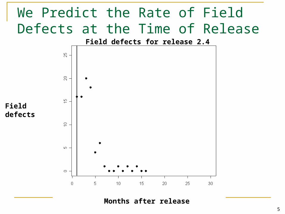
We Predict the Rate of Field Defects at the Time of Release
Months after release
Fielddefects
Field defects for release 2.4
6Months after release
Fielddefects
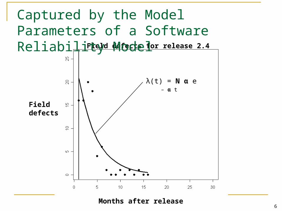
Field defects for release 2.4
Captured by the Model Parameters of a Software Reliability Model
λ(t) = N α e – α t
7Months after release
Fielddefects
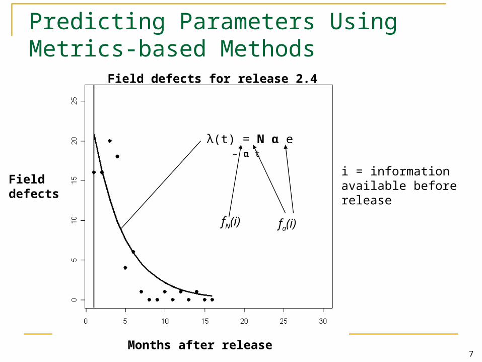
Field defects for release 2.4
Predicting Parameters Using Metrics-based Methods
λ(t) = N α e – α t
i = information available before release
fN(i) fa(i)
8Months after release
Fielddefects
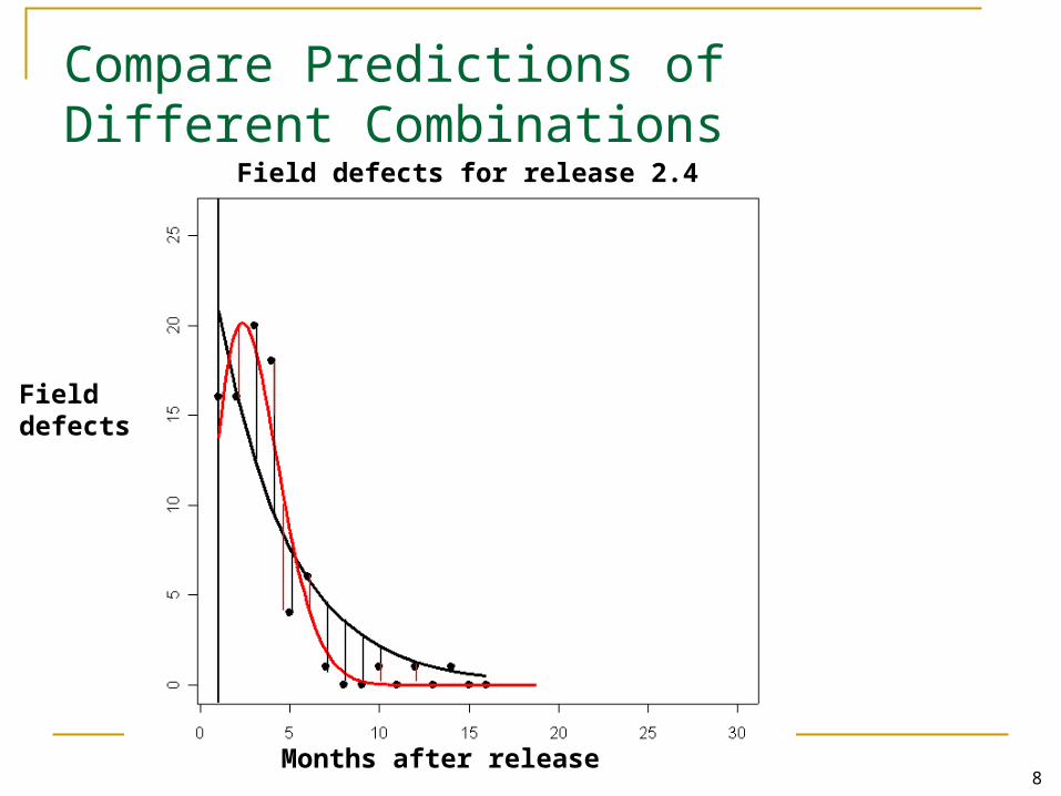
Field defects for release 2.4
Compare Predictions of Different Combinations
9
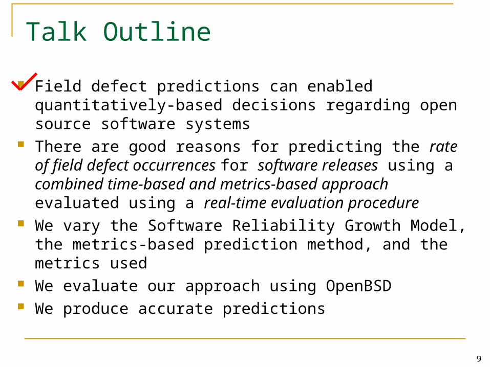
Talk Outline
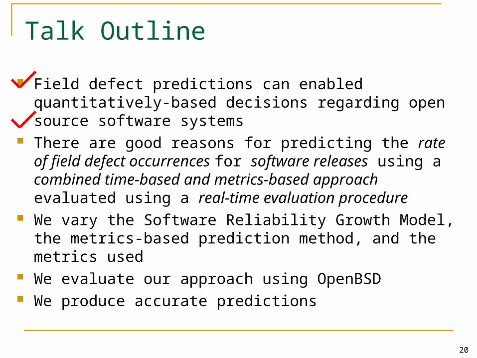
Field defect predictions can enabled quantitatively-based decisions regarding open source software systems
There are good reasons for predicting the rate of field defect occurrences for software releases using a combined time-based and metrics-based approach evaluated using a real-time evaluation procedure
We vary the Software Reliability Growth Model, the metrics-based prediction method, and the metrics used
We evaluate our approach using OpenBSD We produce accurate predictions
10
We Take the Customer’s Perspective
Predicted field defects for Individual software changes (Mockus et al.) Files (Ostrand et al.) Modules (Khoshgoftaar et al.) Entire system (Kenney)
The system is what the customer sees
11
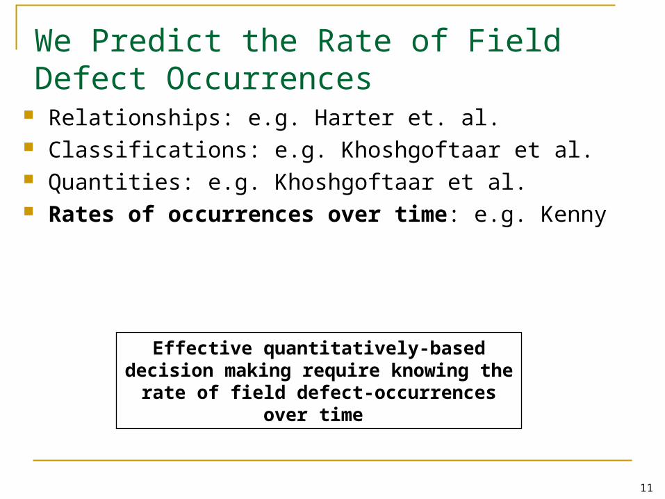
We Predict the Rate of Field Defect Occurrences
Relationships: e.g. Harter et. al. Classifications: e.g. Khoshgoftaar et al. Quantities: e.g. Khoshgoftaar et al. Rates of occurrences over time: e.g. Kenny
Effective quantitatively-based decision making require knowing the rate of field
defect-occurrences over time
12
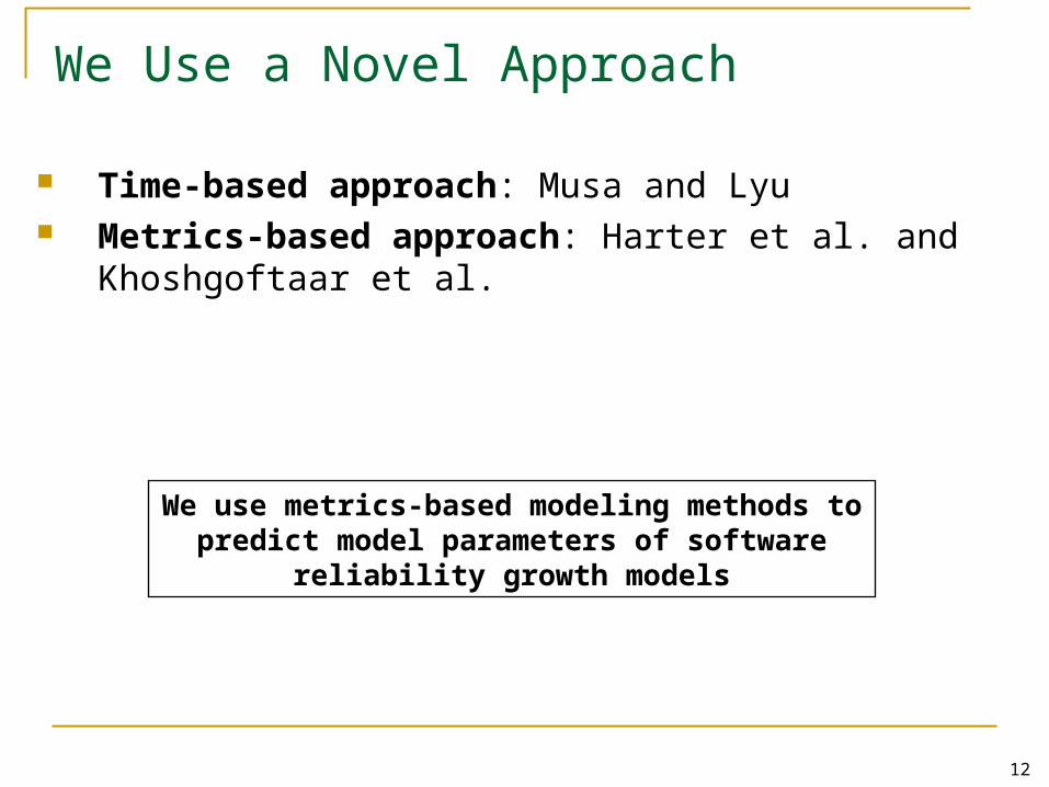
We Use a Novel Approach
Time-based approach: Musa and Lyu Metrics-based approach: Harter et al. and Khoshgoftaar
et al.
We use metrics-based modeling methods to predict model parameters of software reliability
growth models
13
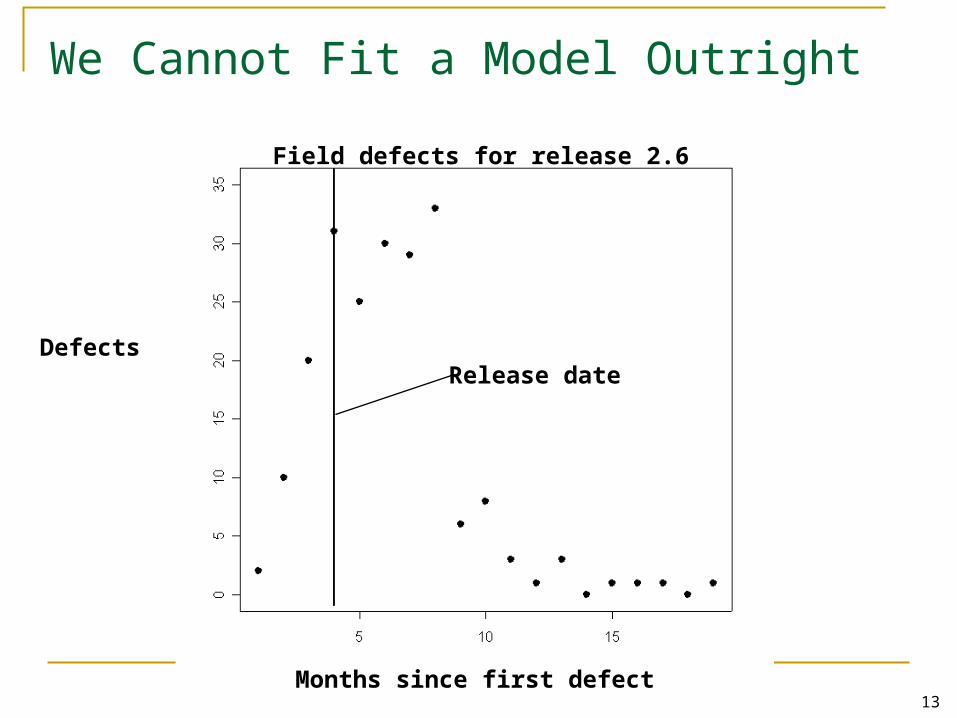
We Cannot Fit a Model Outright
Months since first defect
Release date
Field defects for release 2.6
Defects
14
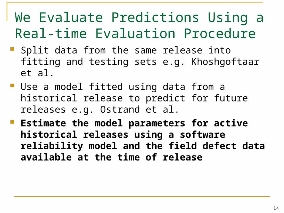
We Evaluate Predictions Using a Real-time Evaluation Procedure
Split data from the same release into fitting and testing sets e.g. Khoshgoftaar et al.
Use a model fitted using data from a historical release to predict for future releases e.g. Ostrand et al.
Estimate the model parameters for active historical releases using a software reliability model and the field defect data available at the time of release
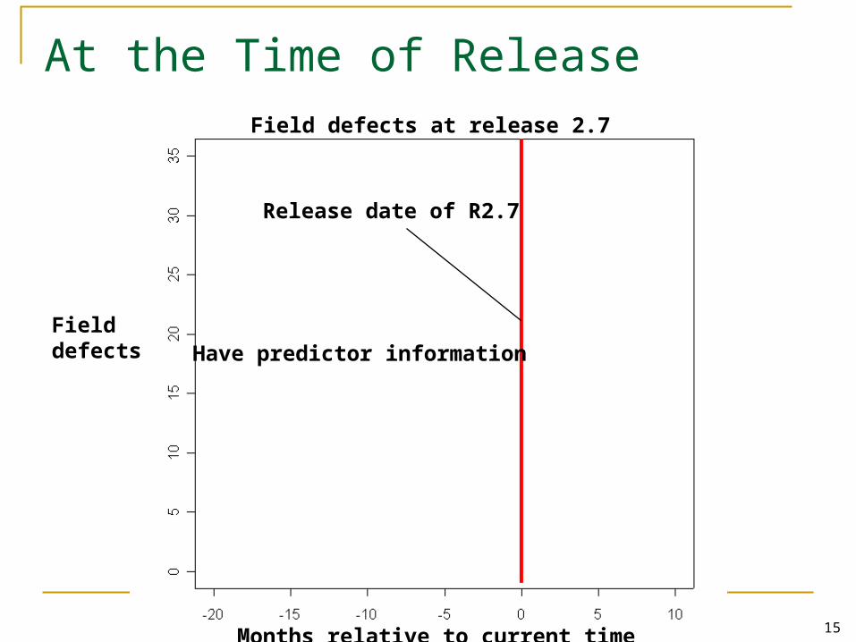
15
At the Time of Release
Release date of R2.7
Have predictor informationField defects
Months relative to current time
Field defects at release 2.7

16
Some Historical Releases
Release date of R2.4
Field defects
Months relative to current time
Field defects at release 2.7
17
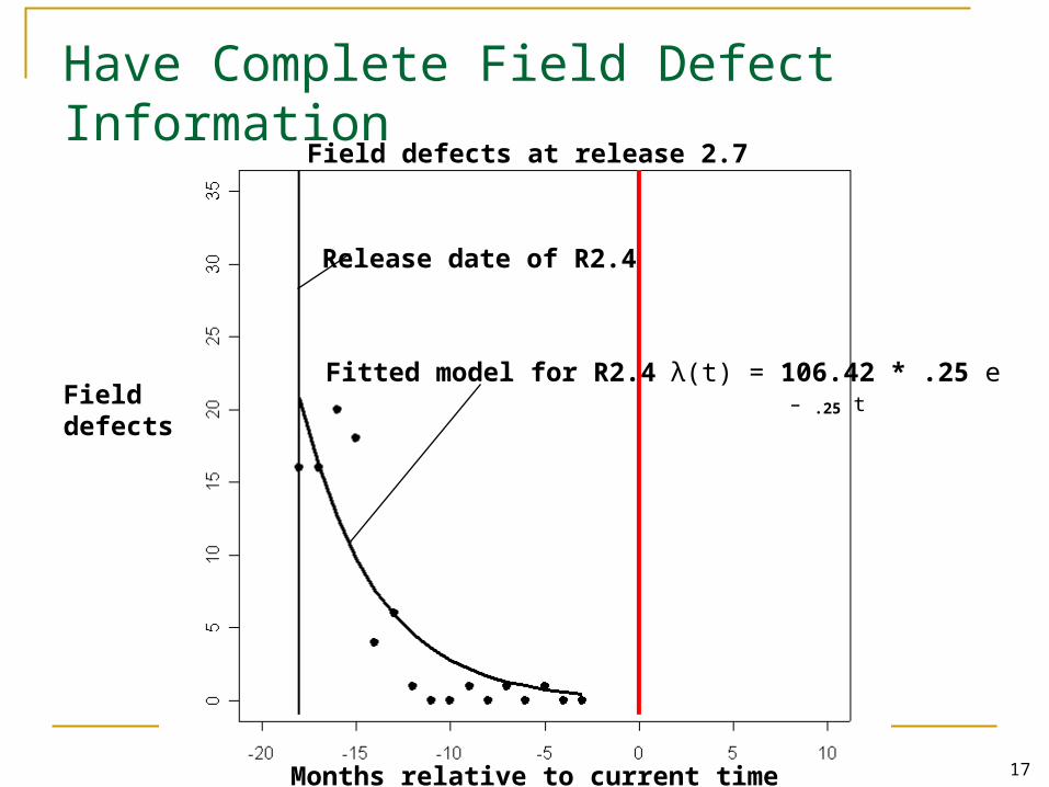
Have Complete Field Defect Information
Release date of R2.4
Fitted model for R2.4 λ(t) = 106.42 * .25 e – .25 t Field defects
Months relative to current time
Field defects at release 2.7
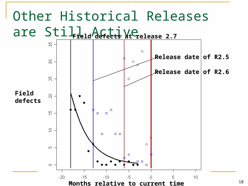
18
Other Historical Releases are Still Active
Release date of R2.5
Release date of R2.6
Field defects
Months relative to current time
Field defects at release 2.7
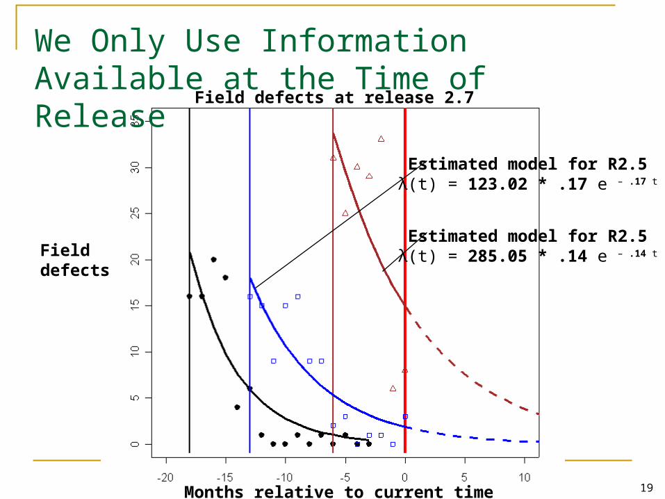
19
We Only Use Information Available at the Time of Release
Field defects at release 2.7
Estimated model for R2.5λ(t) = 123.02 * .17 e – .17 t
Estimated model for R2.5λ(t) = 285.05 * .14 e – .14 tField
defects
Months relative to current time
20
Talk Outline
Field defect predictions can enabled quantitatively-based decisions regarding open source software systems
There are good reasons for predicting the rate of field defect occurrences for software releases using a combined time-based and metrics-based approach evaluated using a real-time evaluation procedure
We vary the Software Reliability Growth Model, the metrics-based prediction method, and the metrics used
We evaluate our approach using OpenBSD We produce accurate predictions
21
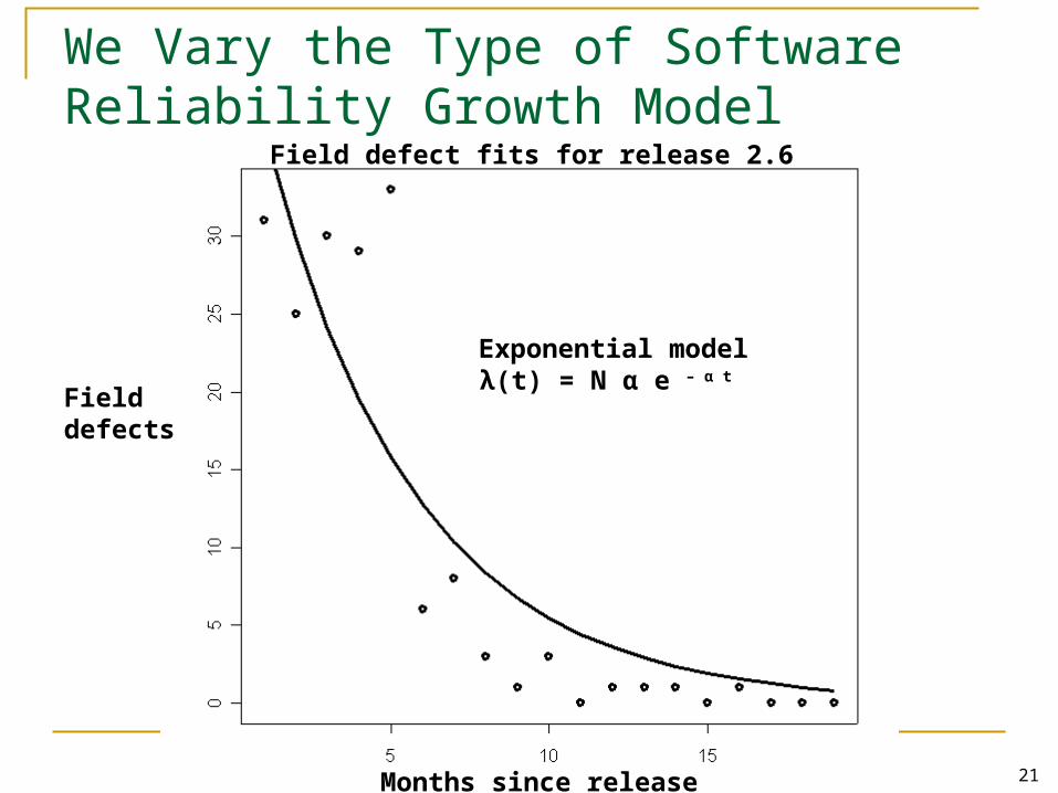
We Vary the Type of Software Reliability Growth Model
Exponential modelλ(t) = N α e – α t
Field defect fits for release 2.6
Field defects
Months since release
22
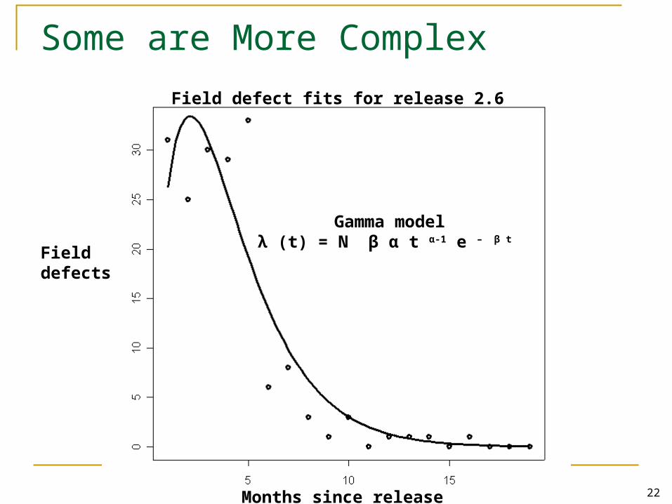
Some are More Complex
Gamma modelλ (t) = N β α t α-1 e – β t
Field defect fits for release 2.6
Field defects
Months since release
23
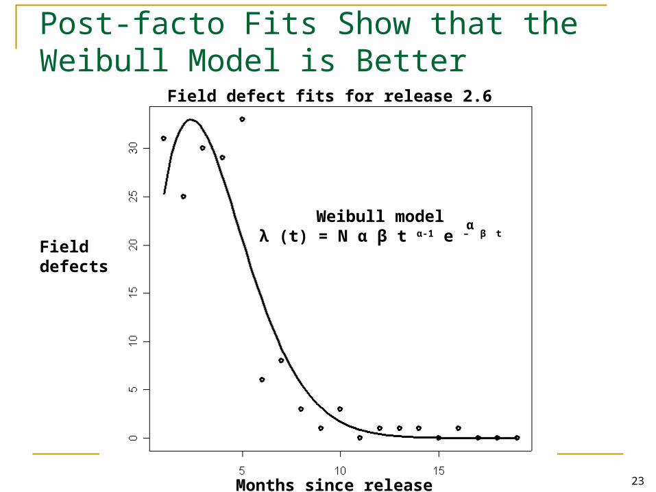
Post-facto Fits Show that the Weibull Model is Better
Weibull modelλ (t) = N α β t α-1 e – β t
α
Field defect fits for release 2.6
Field defects
Months since release
24
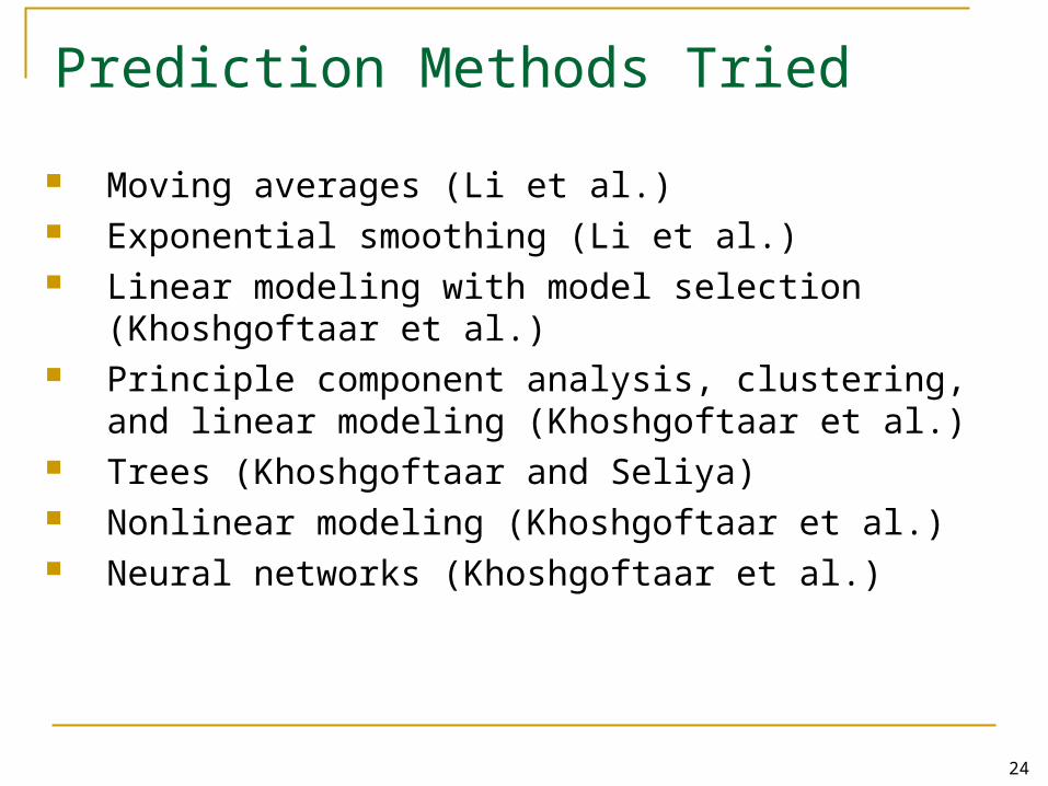
Prediction Methods Tried
Moving averages (Li et al.) Exponential smoothing (Li et al.) Linear modeling with model selection (Khoshgoftaar et
al.) Principle component analysis, clustering, and linear
modeling (Khoshgoftaar et al.) Trees (Khoshgoftaar and Seliya) Nonlinear modeling (Khoshgoftaar et al.) Neural networks (Khoshgoftaar et al.)

25
A Close Look at Moving Averages
Parameter N
R 2.4 R2.5 R2.6
106.4177 123.0219 285.0478
Moving average 1 release: 285.0478
26
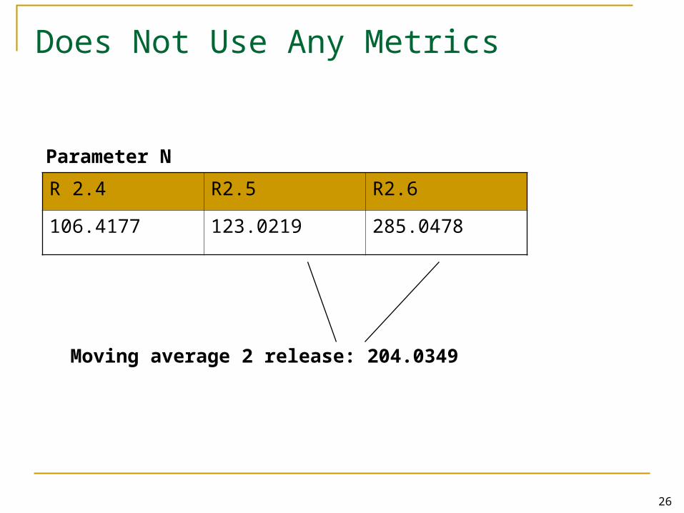
Does Not Use Any Metrics
Parameter N
R 2.4 R2.5 R2.6
106.4177 123.0219 285.0478
Moving average 2 release: 204.0349
27
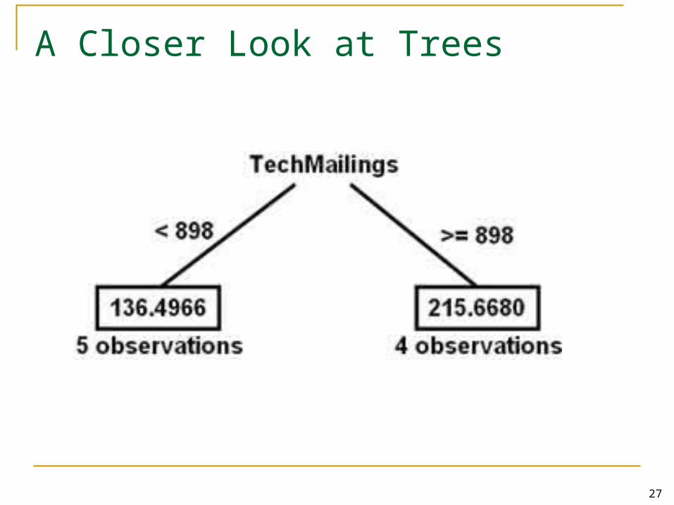
A Closer Look at Trees
28
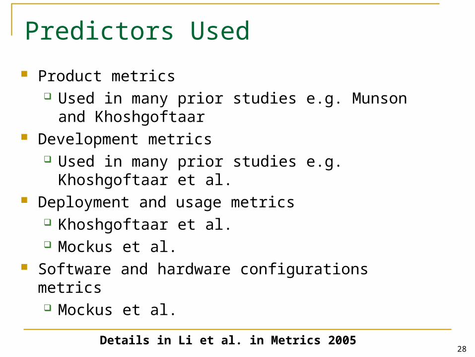
Predictors Used
Product metrics Used in many prior studies e.g. Munson and
Khoshgoftaar Development metrics
Used in many prior studies e.g. Khoshgoftaar et al. Deployment and usage metrics
Khoshgoftaar et al. Mockus et al.
Software and hardware configurations metrics Mockus et al.
Details in Li et al. in Metrics 2005
29
Talk Outline
Field defect predictions can enabled quantitatively-based decisions regarding open source software systems
There are good reasons for predicting the rate of field defect occurrences for software releases using a combined time-based and metrics-based approach evaluated using a real-time evaluation procedure
We vary the Software Reliability Growth Model, the metrics-based prediction method, and the metrics used
We evaluate our approach using OpenBSD We produce accurate predictions
30
OpenBSD
We examine 10 releases (1998-2004) OpenBSD is a Unix like operating system The OpenBSD project uses the Berkley copyrights The OpenBSD project puts out a release approximately
every six months The OpenBSD project uses a CVS code repository The OpenBSD project uses a problem tracking system The OpenBSD project has multiple mailing lists.
31
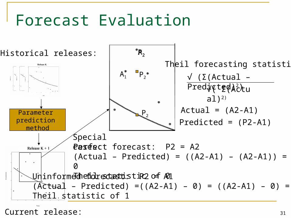
Forecast Evaluation
Parameter prediction
method
Historical releases:
Current release:
Theil forecasting statistic:
√ (Σ(Actual – Predicted)2)
√( Σ(Actual)2)
A1
A2
Actual = (A2-A1)P2
Predicted = (P2-A1)
Perfect forecast: P2 = A2(Actual – Predicted) = ((A2-A1) – (A2-A1)) = 0 Theil statistic of 0
P2
P2
Uninformed forecast: P2 = A1 (Actual – Predicted) =((A2-A1) – 0) = ((A2-A1) – 0) = Actual Theil statistic of 1
Special cases:

32
Talk Outline
Field defect predictions can enabled quantitatively-based decisions regarding open source software systems
There are good reasons for predicting the rate of field defect occurrences for software releases using a combined time-based and metrics-based approach evaluated using a real-time evaluation procedure
We vary the Software Reliability Growth Model, the metrics-based prediction method, and the metrics used
We evaluate our approach using OpenBSD We produce accurate predictions and…
33
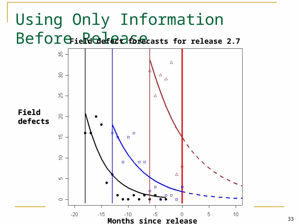
Using Only Information Before Release Field defect forecasts for release 2.7
Field defects
Months since release
Field defects
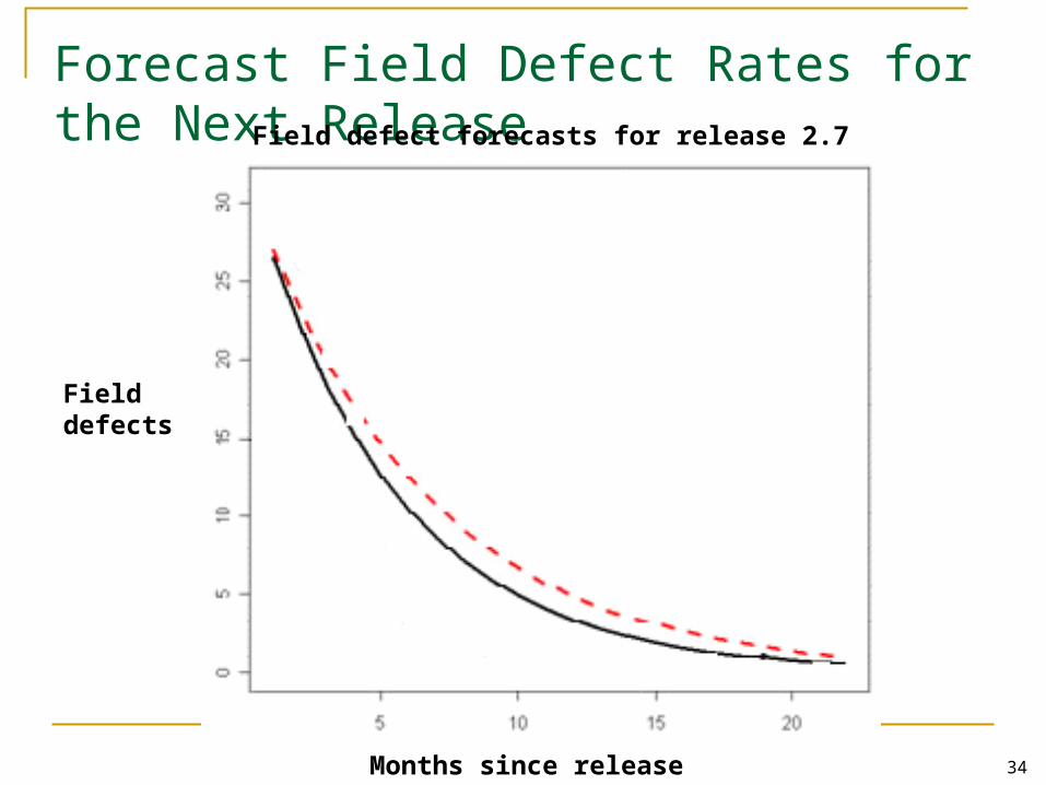
34
Forecast Field Defect Rates for the Next ReleaseField defect forecasts for release 2.7
Field defects
Months since release
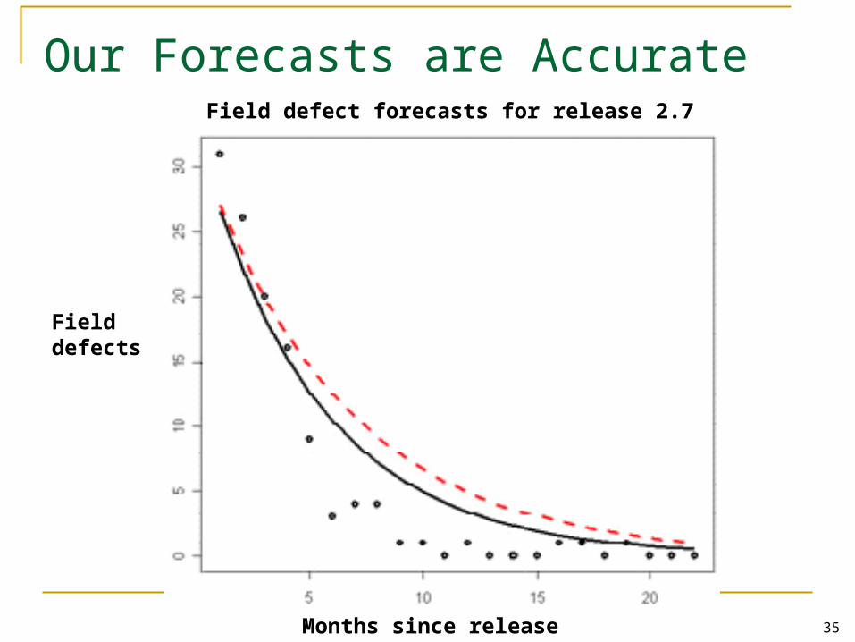
35
Our Forecasts are AccurateField defect forecasts for release 2.7
Field defects
Months since release
36
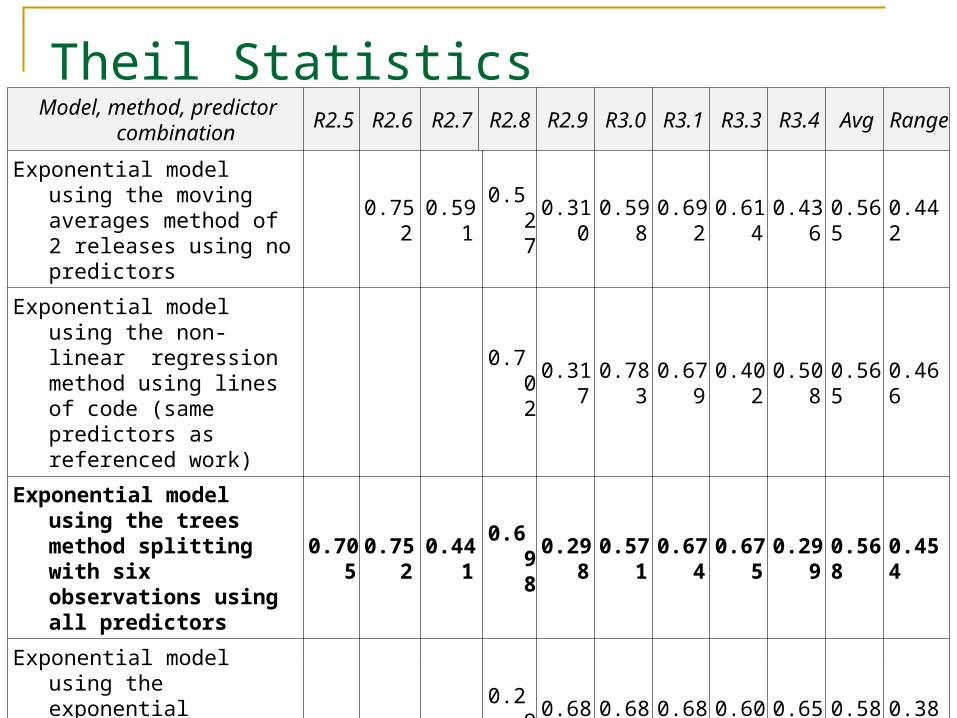
Theil StatisticsModel, method, predictor
combinationR2.5 R2.6 R2.7 R2.8 R2.9 R3.0 R3.1 R3.3 R3.4 Avg Range
Exponential model using the moving averages method of 2 releases using no predictors
0.752 0.591 0.527 0.310 0.598 0.692 0.614 0.436 0.565 0.442
Exponential model using the non-linear regression method using lines of code (same predictors as referenced work)
0.702 0.317 0.783 0.679 0.402 0.508 0.565 0.466
Exponential model using the trees method splitting with six observations using all predictors
0.705 0.752 0.441 0.698 0.298 0.571 0.674 0.675 0.299 0.568 0.454
Exponential model using the exponential smoothing method of five releases using no predictors
0.297 0.680 0.680 0.686 0.606 0.655 0.585 0.388
Gamma model using the non-linear method using lines of code (same predictors as referenced work)
0.669 0.405 0.706 0.659 0.439 0.641 0.587 0.354

37
Exponential Model Produces Better Results
9 out of the 10 best methods ranked by average Theil use the Exponential model
38
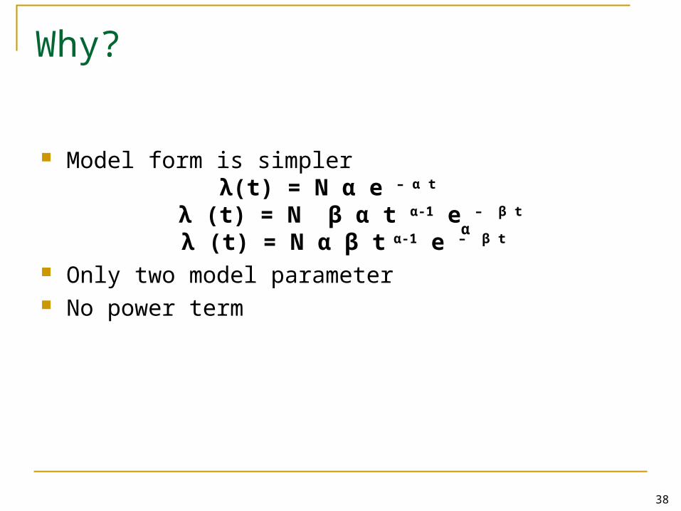
Why?
Model form is simplerλ(t) = N α e – α t
λ (t) = N β α t α-1 e – β t
λ (t) = N α β t α-1 e – β t
Only two model parameter No power term
α
39
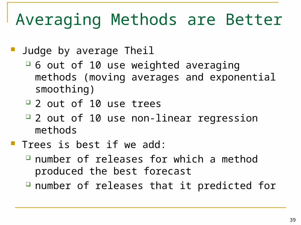
Averaging Methods are Better
Judge by average Theil 6 out of 10 use weighted averaging methods (moving
averages and exponential smoothing) 2 out of 10 use trees 2 out of 10 use non-linear regression methods
Trees is best if we add: number of releases for which a method produced the
best forecast number of releases that it predicted for
40
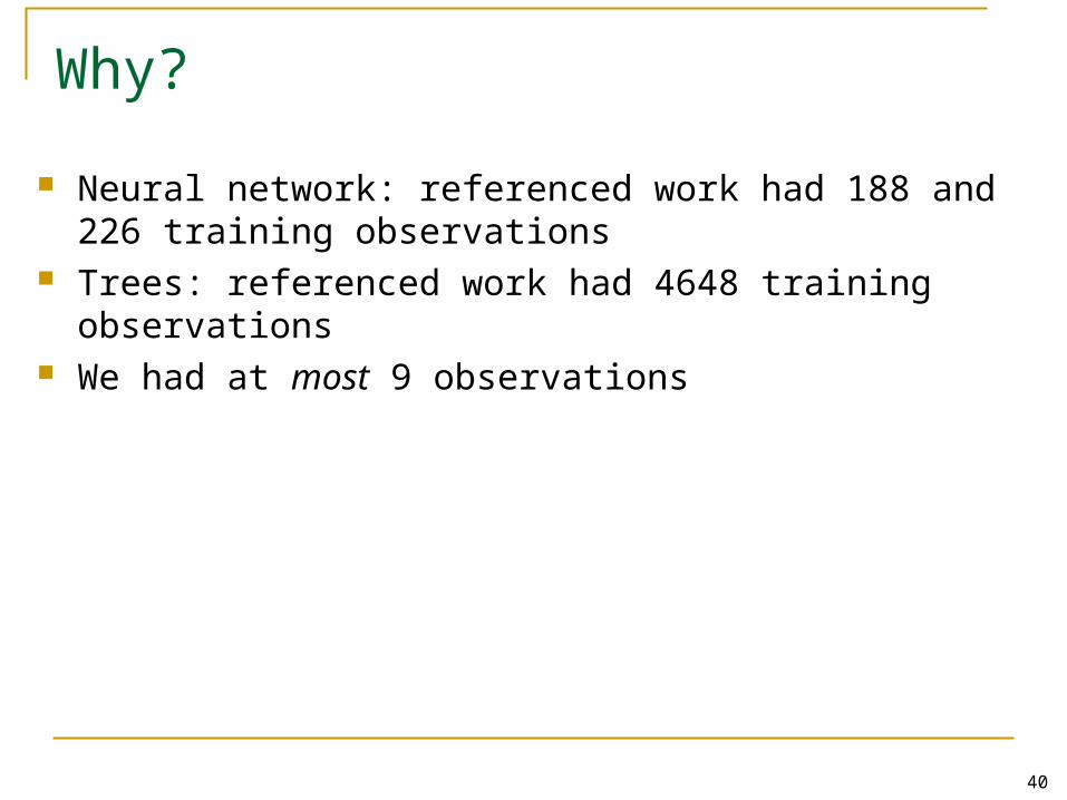
Why?
Neural network: referenced work had 188 and 226 training observations
Trees: referenced work had 4648 training observations We had at most 9 observations
41
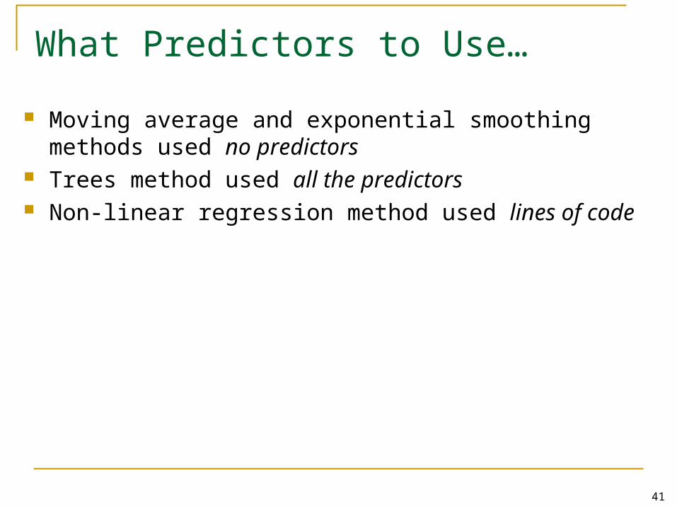
What Predictors to Use…
Moving average and exponential smoothing methods used no predictors
Trees method used all the predictors Non-linear regression method used lines of code
42
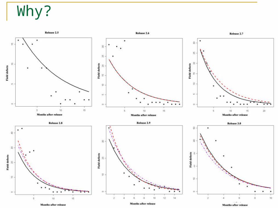
Why?
43
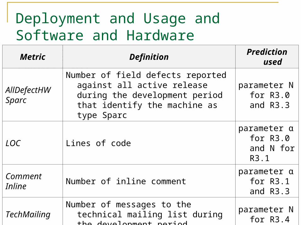
Deployment and Usage and Software and Hardware Configuration Metrics are ImportantMetric Definition Prediction used
AllDefectHWSparc
Number of field defects reported against all active release during the development period that identify the machine as type Sparc
parameter N for R3.0 and R3.3
LOC Lines of codeparameter α for
R3.0 and N for R3.1
CommentInline
Number of inline commentparameter α for
R3.1 and R3.3
TechMailingNumber of messages to the technical mailing list
during the development periodparameter N for
R3.4
NotCUpdateNumber of updates (deltas) to files that are not c
source files during the development periodparameter α for
R3.4
44
Talk Outline
Field defect predictions can enabled quantitatively-based decisions regarding open source software systems
There are good reasons for predicting the rate of field defect occurrences for software releases using a combined time-based and metrics-based approach evaluated using a real-time evaluation procedure
We vary the Software Reliability Growth Model, the metrics-based prediction method, and the metrics used
We evaluate our approach using OpenBSD We produce accurate predictions and…
45
Where to Go From Here?
Validate results using: Commercial systems Other open source systems
Update predictions as more data becomes available: Bayesian approach (Liu et al.) U-plot (Brocklehurst and Littlewood)
Case studies applying our technique

46
Forecasting Field Defect Rates Using a Combined Time-based and Metrics-based Approach: a Case Study of OpenBSD
Paul Luo LiJim HerbslebMary ShawCarnegie Mellon University