1

Extended Instrumental Variables Estimation for Overall Effects

Marshall M. Joffe

Dylan Small

Steven Brunelli

Thomas Ten Have

Harold I. Feldman

1 Introduction

Instrumental variables (IV) methods have been used successfully to control for

confounding in a number of settings in which conventional methods fail (Davey and Ebrahim

2003;Mark and Robins 1993;McClellan and Newhouse 1997). IV methods may be used in

estimating the component and joint effects of multiple treatments or exposures (Stock 2001).

However, when one of the treatments under study affects another, IV methods will not by

themselves provide valid estimates of the overall effect of the former. We consider extension of

IV methods that allow estimation of the overall effects of the initial treatment.

For motivation, we consider estimating the overall effects of type of vascular access (VA)

among hemodialysis (HD) patients on clinical outcomes; e.g., mortality. VA can affect the dose

of dialysis received (Sehgal et al. 1998;Dhingra, Young, Hulbert-Shearon, Leavey and Port

2001). The clinical center at which dialysis is provided may be a good instrument for the joint

effects of VA and dose, but, as we will argue, it is not an instrument for the overall effect of VA.

We will thus need to use extended IV methods.

This manuscript is organized as follows. First, we consider the VA problem in more

detail. Then, using both graphical and counterfactual approaches to causality, we show how,

under our assumptions, IV methods are appropriate for estimating the component and joint

effects of VA and dose (the earlier and later treatments), but not the overall effect of VA (the

earlier treatment). We then show how to estimate the overall effect, and consider extensions to

situations with confounders or additional mediators of the effect of the instrument, to failure-time

outcomes, and to time-varying auxiliary treatments.

2 Vascular access in hemodialysis

Hemodialysis (HD) is one of the principal modalities of renal replacement therapy in end-

stage renal disease (ESRD), a condition in which a person’s kidneys no longer function

adequately. In HD, blood is removed from the body, filtered, and then returned to the vascular

system. This process requires access to the vascular system. This access can take the form of a

catheter, implantation of synthetic material between an artery and vein (graft), or a native

arteriovenous fistula.

The type of VA can impact the dose of dialysis that can be delivered, and so can influence

the dose of dialysis actually received. VA may influence clinical outcomes, including mortality

(Dhingra et al. 2001;Wolfe, Dhingra, Hulbert-Shearon, Leavey and Port 2000). A good part of

the effect of VA may be mediated by delivered dialysis dose. Type of VA may affect clinical

outcomes by other pathways as well.

In ESRD, many of the treatments used to treat various aspects of ESRD or its

consequences are subject to confounding by indication (Feldman et al. 2004;Reddan et al. 2002);

i.e., subjects with an indication for a particular treatment often have more severe disease than

other subjects . There are a number of reasons that patients who receive dialysis catheters may

be sicker than those who are treated via fistula or graft. Fistula/graft creation requires vascular

surgery, and patients with more comorbid disease may often are not surgical candidates. In

addition, fistulas and grafts require suitably healthy vascular systems, which may not be present

in older, frailer patients or those with extensive cardiovascular disease. Finally, grafts (and

particularly) fistulas require time to mature after they are placed and before they are ready for

use, whereas catheters are ready instantaneously upon placement. Patients with less access to

health care, and who therefore are less likely to receive care for other diseases, are less likely to

present in time to receive fistulas or grafts, and more likely to receive catheters.

Confounding by indication is often difficult to control analytically using standard

methods, e.g., regression. IV analysis provides an alternative approach to controlling

confounding. For this method to work, the instrumental variable should be related to the

outcome only through its effect on the treatment(s) of interest. The center at which dialysis is

provided is a plausible candidate for an instrument. The choice of center for dialysis patients

might be expected to be driven primarily by factors not intimately related to prognosis, such as

geographical proximity of the patient to the center. Inasmuch as center is not strongly associated

with prognosis, except through its effect on the treatments of interest, center may fulfill this

criterion for an instrumental variable; this criterion has implicitly been used to provide causal

interpretation to associations between average levels of compliance within centers to guidelines

about dialysis dose and hematocrit with center-specific mortality (Wolfe, Hulbert-Shearon,

Ashby, Mahadevan and Port 2004). For similar reasons, we propose using practice as an

instrument for estimating the effect of VA type on outcome.

3 The effect of vascular access

To define our problem, it is useful to consider the various pathways by which the primary

treatment (VA) might affect clinical outcomes, and other ways associations between the primary

treatment and outcome might be generated. Causal diagrams (Pearl 1995;Pearl 2000) are useful

for this purpose. We will consider these diagrams together with formal definitions of effects

based on the potential outcomes model (Rubin 1974;Rubin 1978;Neyman 1990).

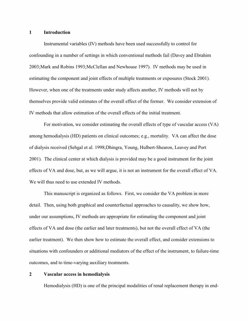
We begin with a simple diagram showing relations between the main variables of interest

(figure 1). Let A denote the primary treatment (type of VA), S denote the auxiliary treatment

(dose of dialysis), and Y the clinical outcome of interest (e.g., mortality). We presume that A

affects S; thus we draw an arrow from A to S ( ); the auxiliary treatment (dialysis dose) may

affect clinical outcomes ( ). Further, the primary treatment may affect clinical outcomes

directly (i.e., through pathways not containing S); thus, we also draw an arrow .

The overall impact of the primary treatment (VA) on clinical outcomes is represented by

considering both paths from A to Y (i.e., and ). The direct effect of the primary

treatment (VA), controlling for the auxiliary treatment (dialysis dose), is represented by the path

; the indirect effect is represented by the path . In our example, because VA can

determine the dose of dialysis, the indirect path cannot be ignored in assessing the

impact of VA on outcome.

We supplement the causal diagrams with a potential outcomes approach to more formally

define overall, direct, and indirect effects (Pearl 2001;Robins and Greenland 1992). Let

denote the outcome that would be seen in a subject were that person to receive level a of the

primary treatment and level s of the auxiliary treatment. denotes the value that S would

assume were treatment level a provided, without S being manipulated by the investigator. is

the outcome that would be seen were the investigator to provide primary treatment a but leave

the choice of S subject to the same possibly unknown factors governing it during the study; thus,

under a consistency assumption (Robins and Rotnitzky 2004), . Overall effects of A are

contrasts of and , . The direct effect of A is a contrast of and ; i.e, a

contrast of outcomes holding s physically constant but varying a. There are several direct effects,

depending on the choice of s. Prescriptive direct effects require prespecification of s; for natural

direct effects, s is the value it would assume under a reference level of the primary treatment

A; i.e., . Natural indirect effects are contrasts of and ; i.e., allow S to vary as

it would by varying A, but fix A to some common value. There is no nonparametric definition of

prescriptive indirect effects, although there are several definitions based on parametric models

(MacKinnon, Lockwood, West and Sheets 2002).

In our example, because the type of access determines to a degree the possible dose of

dialysis, in determining the impact of VA, we cannot simply control or adjust for dose. Thus, we

will concentrate on estimating the overall impact of VA. However, the direct and indirect effects

will be of interest, not only for mechanistic understanding and explanation, but also for deriving

estimates of the overall effect.

4 Identification and Estimation

To understand appropriate approaches for estimation, we supplement the causal diagram

(figure 1) with other variables. In particular, we add both measured (X) and unmeasured (U)

confounders of the effect of A and S; X and U influence A, S, and Y. The presence of unmeasured

confounders makes standard adjustments for confounders X inadequate for estimating the effects

of A and S. We also add a node for an instrumental variable (IV) R, whose association with

outcome is presumed to be solely due to its effect on A and S. As with other IVs, R influences

treatment (A and S), but has no direct effect on Y (no arc; i.e., an exclusion restriction

(Angrist, Imbens and Rubin 1996) holds), and there are no unmeasured common causes of R and

Y. Figure 2 represents these relationships.

In this setup, R is an instrument for the joint effects of A and S but not for the overall

effect of A. To see this, note that d-separates R from Y, and is affected by R; R then

satisfies graphical criteria (Pearl 2000) but not necessarily standard econometric criteria for an

instrument . Suppose we assume a linear, no interaction model for the effect of A and S on Y:

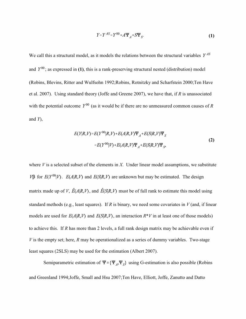
We call this a structural model, as it models the relations between the structural variables

and ; as expressed in (1), this is a rank-preserving structural nested (distribution) model

(Robins, Blevins, Ritter and Wulfsohn 1992;Robins, Rotnitzky and Scharfstein 2000;Ten Have

et al. 2007). Using standard theory (Joffe and Greene 2007), we have that, if R is unassociated

with the potential outcome (as it would be if there are no unmeasured common causes of R

and Y),

where V is a selected subset of the elements in X. Under linear model assumptions, we substitute

for . and are unknown but may be estimated. The design

matrix made up of V, , and must be of full rank to estimate this model using

standard methods (e.g., least squares). If R is binary, we need some covariates in V (and, if linear

models are used for and , an interaction R*V in at least one of those models)

to achieve this. If R has more than 2 levels, a full rank design matrix may be achievable even if

V is the empty set; here, R may be operationalized as a series of dummy variables. Two-stage

least squares (2SLS) may be used for the estimation (Albert 2007).

Semiparametric estimation of using G-estimation is also possible (Robins

and Greenland 1994;Joffe, Small and Hsu 2007;Ten Have, Elliott, Joffe, Zanutto and Datto

(1)

(2)

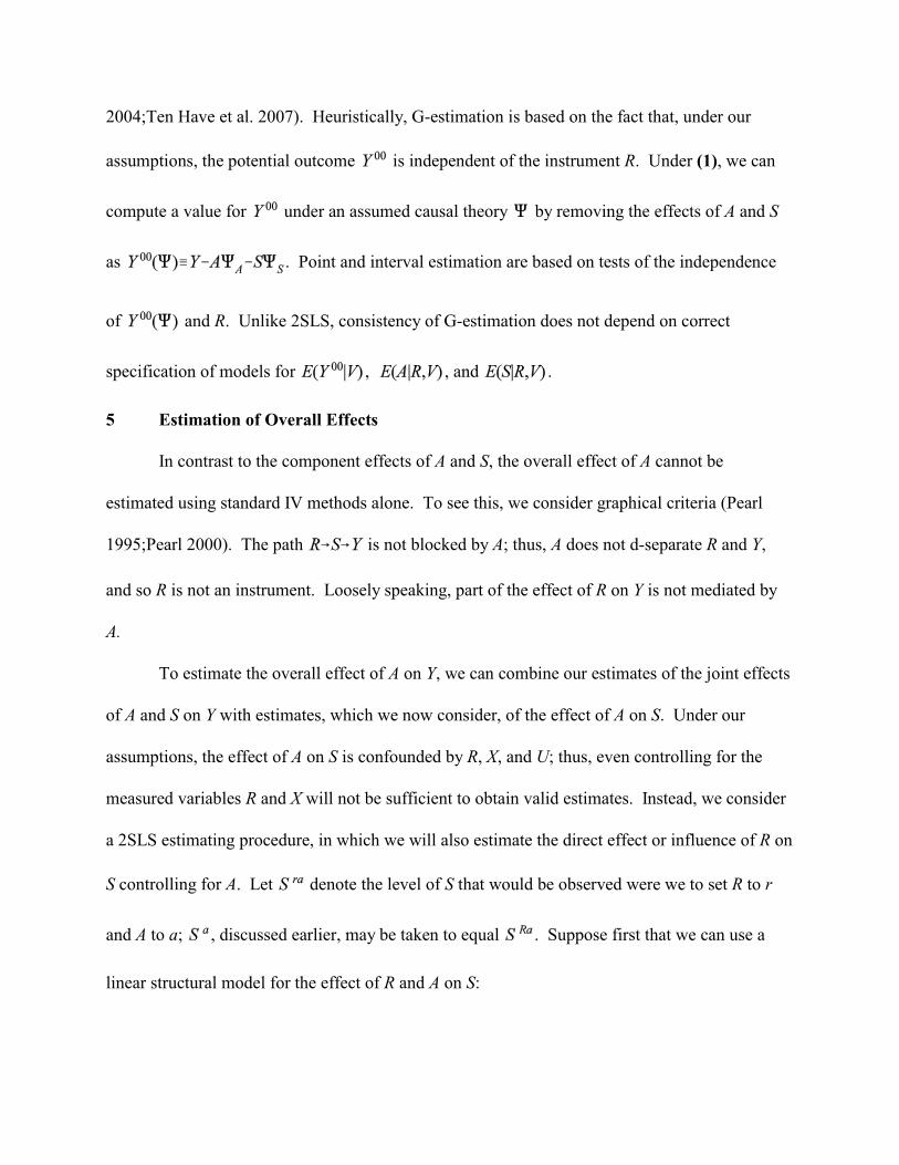
2004;Ten Have et al. 2007). Heuristically, G-estimation is based on the fact that, under our

assumptions, the potential outcome is independent of the instrument R. Under (1), we can

compute a value for under an assumed causal theory by removing the effects of A and S

as . Point and interval estimation are based on tests of the independence

of and R. Unlike 2SLS, consistency of G-estimation does not depend on correct

specification of models for , , and .

5 Estimation of Overall Effects

In contrast to the component effects of A and S, the overall effect of A cannot be

estimated using standard IV methods alone. To see this, we consider graphical criteria (Pearl

1995;Pearl 2000). The path is not blocked by A; thus, A does not d-separate R and Y,

and so R is not an instrument. Loosely speaking, part of the effect of R on Y is not mediated by

A.

To estimate the overall effect of A on Y, we can combine our estimates of the joint effects

of A and S on Y with estimates, which we now consider, of the effect of A on S. Under our

assumptions, the effect of A on S is confounded by R, X, and U; thus, even controlling for the

measured variables R and X will not be sufficient to obtain valid estimates. Instead, we consider

a 2SLS estimating procedure, in which we will also estimate the direct effect or influence of R on

S controlling for A. Let denote the level of S that would be observed were we to set R to r

and A to a; , discussed earlier, may be taken to equal . Suppose first that we can use a

linear structural model for the effect of R and A on S:

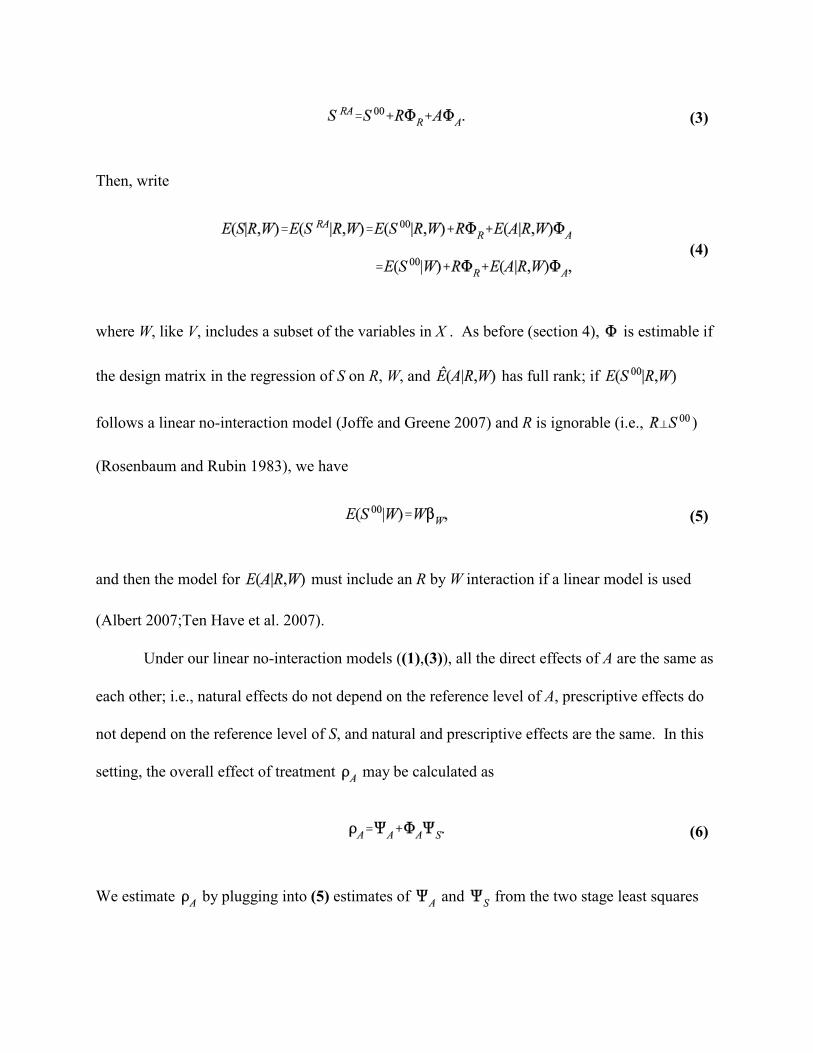
Then, write

where W, like V, includes a subset of the variables in X . As before (section 4), is estimable if

the design matrix in the regression of S on R, W, and has full rank; if

follows a linear no-interaction model (Joffe and Greene 2007) and R is ignorable (i.e., )

(Rosenbaum and Rubin 1983), we have

and then the model for must include an R by W interaction if a linear model is used

(Albert 2007;Ten Have et al. 2007).

Under our linear no-interaction models ((1),(3)), all the direct effects of A are the same as

each other; i.e., natural effects do not depend on the reference level of A, prescriptive effects do

not depend on the reference level of S, and natural and prescriptive effects are the same. In this

setting, the overall effect of treatment may be calculated as

We estimate by plugging into (5) estimates of and from the two stage least squares

(3)

(4)

(5)

(6)

(2SLS) approach in Section 4 and from the two stage least squares approach in this section,

and call this the extended 2SLS estimate. Standard errors for the extended 2SLS estimates of

may be calculated analytically, or using a nonparametric bootstrap. Appendix 1 provides analytic

formulas for the standard errors from the extended 2SLS approach, and compares these to a

three-stage least squares (3SLS) approach, which can be more efficient under certain conditions.

6 Simulation Study:

We performed a small simulation study to examine the properties of the various

estimators. Consider a setting where W consists of two variables that are generated as

independent standard normals, there are 500 subjects and the parameters are the following (see

Appendix 1 for definitions of and ).: , , , , ,

, , , , . The total effect of A is

.

Table 1 shows the bias and root mean square error of the path analysis estimate of the

effect of A (which assumes no unmeasured confounding), the estimate of the total effect of A

based on two stage least squares, and the estimate of the total effect of A based on three stage

least squares in 2000 simulations. The 2SLS and 3SLS estimates performed virtually identically.

The coverage of the 95% confidence intervals based on from the simulation study was

0.9500 for the 2SLS approach and 0.9485 for the 3SLS approach.

The 3SLS estimates can provide efficiency gains in other situations in which different

instruments are used for S compared to Y (this is analogous to the fact that seemingly unrelated

regression (SUR) provides efficiency gains when the different equations have some different

covariates, whereas SUR provides no efficiency gains if all the equations have exactly the same

covariates). If we use the same simulation setting as above but assume that the second

component of W is an instrument for S but not Y and let , then the estimation results

are shown in the second scenario in table 1. The root mean squared error of the 3SLS estimate is

24% less than that of the 2SLS estimate for this scenario.

7 Extensions:

We consider four extensions to this framework:

1. the presence of confounders of the effect of R on Y;

2. the presence of additional measured mediators of the “effect” of R on Y;

3. the use of failure-time outcomes instead of outcomes measured at a fixed time; and

4. settings in which the intermediate S is not fixed but rather time-varying.

7.1 Confounders of the instrument

Until now, we have supposed that associations between the instrument and outcome can

be explained fully in terms of the associations of the instrument with the specified treatments A

and S and the effects of those treatment on the outcome. In this and the following subsection, we

weaken this requirement by allowing the instrument R to be associated with some other variable

associated with the outcome. In some cases, this variable will be a confounder of the effect of R;

in others an intermediate treatment on a path from R to Y not involving A or S.

Suppose first that there are individual characteristics X which are associated with the

instrument and the outcome (figure 3). For example, it is possible that patients initiating dialysis

at some centers are sicker, have higher income or education, or are older than patients initiating

dialysis at other centers. These associations may lead to associations between the putative

instrument R and outcome Y even in the absence of any effects of the treatments A and S on Y.

For estimation, the same extended 2SLS approach taken previously is appropriate here, so

long as appropriate confounders of the associations of the instrument R with Y and S are

considered in the appropriate models. In particular, the effects of A and S on Y are estimable

using (2) so long as ; that is, if R is an instrument for the effects of A and S

conditional on V. Thus, any common causes of R and must be included in V . Similarly, the

effect of A on S is estimable using (4) and (5) if those models are correctly specified and there are

no unmeasured common causes of R and ; here, all measured common causes of R and S

must be included in W.

7.2 Additional mediators of the effect of the instrument

In our motivating example, center (R) is associated with a variation in a wide range of

treatment patterns. For example, practice may affect dosing of erythropoetin and intravenous

iron, both of which are used for treating the anemia prevalent among HD patients and which may

affect other clinical outcomes, including mortality. Q denotes these additional mediating

variables. We augment our causal graph to show these additional paths from R to Y, as well as

paths from U and X to R (figure 4). The approach sketched below will also be appropriate if Q

affects A and S (i.e., additional arcs and are added to figure 4).

For estimation, we augment our causal model (1) with a term for the effect of Q:

This again implies that

Estimation can again proceed using 2SLS; we now require that the design matrix comprised of V,

, , and have full rank. Estimating the effect of A on S can proceed as

previously, as can combining inferences for the overall effect from the models for S and Y.

The approach above allows as a special case. In this setting, the assumption of no

direct effect of the instrument (i.e., no effect not explained by the measured variables (here A and

S)) is equivalent to in (8) and so may be tested by testing . This estimation and

testing may be problematic where R consists of many unordered categories and so the dimension

of is high, as in our example.

7.3 Failure-time outcomes

In our motivating example, death is common, and time to death is arguably the most

important outcome. Our system of linear models will not work for the popular but nonlinear Cox

proportional hazards model (Cox 1972), but the approach can apply to the accelerated failure-

time model (AFTM), which is a linear model for the natural logarithm of the failure-time (Cox

and Oakes 1984). Henceforth, we use Y to denote the log of the failure-time.

In almost any study with failure-time outcomes, the failure-time will sometimes be

censored. This complicates application of the methods discussed above, as expectations

cannot be calculated using least squares. This leaves two alternatives for estimation: 1) assume a

(7)

(8)

parametric form or distribution for the error in , or use a semiparametric G-estimation

approach. Both approaches require appropriate ways to deal with censoring. We consider here

two types of censoring: fixed (modified type I censoring) and “random” censoring. The first

refers to planned censoring, where a potential censoring time is known for all subjects, regardless

of whether a censoring event is actually observed. Random censoring refers to loss to follow-up

or other reasons for unplanned or unpredictable censoring.

For fixed censoring, one must use artificial censoring (Joffe and Brensinger 2001;Robins

1992;Robins et al. 1992) in the analysis. Artificial censoring results in difficulties in estimating

the structural parameters due in part to the fact that the function to be optimized is no longer

continuous. This complicates obtaining both point and interval estimates. Random censoring

can be dealt with using inverse probability of censoring weighting methods (Robins et al. 1992);

these methods rely on the censoring process being ignorable given the measured past.

7.4 Time-varying auxiliary treatments

In many cases, both main and auxiliary treatments may vary over time. In our example,

both VA and dialysis dose may vary within an individual. Nonetheless, the type of VA may vary

less frequently (as some surgical procedure is required to establish VA), and so we make the

working assumption that VA is constant over an extended period, while dialysis dose may vary

over time. In this setting, it is appealing to consider modeling the effect of the auxiliary

intervention received at each point in time, then incorporating these effects into estimates of the

overall effect of the main intervention. We consider briefly how to extend our approach to this

setting.

Let denote the level of S that applies at each discrete time t, and let denote the entire

history of S. Consider first a model for the joint effects of A and S on Y; a fairly general linear

model is

The 2SLS approach (2) then becomes

to estimate distinct parameters, we will need the design matrix formed from each of the

individual elements in regression (10) to be full rank. Collinearity may be a severe problem if, as

expected, the effect of R on the various 's is similar. Dimension reduction may be helpful here;

suppose that is a low-dimension function of . The simplest such function is , a

common value for all t.

Estimating the effect of A on S requires less modification; (3) generalizes to

and (4) becomes

One can fit a separate model for each , or one can model various 's jointly with a common

parameter , where the time-specific parameters are functions of . In the latter

case, one will need to account for the nonindependence of the various 's in an individual in the

(9)

(10)

(11)

(12)

variance calculation.

It is easy to show that, generalizing (6), the overall effect may be calculated as

Variance calculations can be based on generalizations of the 2SLS or 3SLS estimators considered

in the appendix. One can also use semiparametric G-estimators for and .

Estimation for failure-time outcomes with multiple measurements of the auxiliary

treatment S is more complicated. Estimating the separate component effects of A and S is

straightforward, using G-estimation. However, estimation of the overall effect of A under IV-like

assumptions is problematic.

To estimate the component effects of A and S, we use a structural nested failure-time

model (SNFTM). Let denote the level of S that applies at time t measured in continuous

time; we presume that is constant on the interval between discrete measurement times t.

The simplest SNFTM for this setting is an AFTM with time-varying covariates:

Model (14) assumes no interaction between A and . For a time-invariant , this reduces

to the standard AFTM. Estimation can use G-estimation, which is based on testing the

independence of and R; for model (14), this will require a 2

(13)

(14)

degree of freedom test.

Estimation of the effect of A on S can also use a generalization of the method sketched

above. For now, we assume that, even though S may vary over time, the effect of A on S is

constant on average; i.e., in (11), , a constant.. We can use 2SLS or G-estimation

methods to estimate . As before, the overall effect can be estimated as .

Inference under less restrictive assumptions is more complicated. Consider model (11)

without the restriction of constant effects. We no longer have available a simple formula for

obtaining overall effects. Let overlines denote the history of a variable over time; thus,

denotes the history of . To obtain overall effects, one could in principle compute

from the data and models for the effect of A and S on Y and for the effect of A on S. One

could then compare with at an individual level, or average over a

population, as a measure of overall effects. Let denote the history of S that

would be seen by following the observed history through t, then setting thereafter. One

could in principle make this comparison by “blipping-up;” i.e., recursively computing

from , , and using a rank-preserving structural nested model. Unfortunately,

for a given individual, will only be computable if is observed; if a subject fails before t

and is no longer observable, as would be true if Y refers, even in part, to mortality, will

not be observable for . If the treatment A is beneficial overall at each point in time, so

that , there will be some times t for which we cannot compute for some subjects. If

the treatment is consistently harmful or failure never precludes observation of S subsequently,

this approach can be used together with the restrictive assumption of rank-preservation.

Appropriate coding of a so that large a is beneficial can finesse this issue.

8 Discussion

We have sketched an approach for estimating the overall effect of an exposure or

treatment in settings in which conventional analysis fails because of unmeasured confounders.

Here, IV-type assumptions may be valid for estimating the joint effects of the main and auxiliary

treatments, but are not by themselves sufficient to identify the overall effect of the main

treatment. So long as we can estimate the effect of the main treatment on the auxiliary one, we

will be able to estimate the overall effect.

While the relaxation of the no-unmeasured confounders assumption is valuable, we have

needed to substitute other assumptions. These assumptions include structural assumptions and

modeling assumptions. The structural assumptions include: 1) the assumption that there are no

effects of the IV on the main outcome except those mediated by measured variables (although

this assumption is relaxed in 7.2), and 2) the assumption that the effect of the study treatment is

deterministic (i.e., given one counterfactual and the true model, we could recover any other

without error). Neither assumption is fully testable (Robins et al. 1992;Robins 1994).

The assumption of deterministic treatment effects, roughly equivalent to rank-

preservation, is often a heuristic for deriving and explaining estimation procedures, but may

impose no restrictions on the joint distribution of the observables when compared with the less

restrictive structural distribution models (Robins et al. 1992); in these settings, analyses which

heuristically assume rank preservation can be useful (Robins et al. 1992) (Ten Have et al. 2007).

While this is true in the simpler settings in which both treatments are scalar, it is not true in

general when the outcome is a failure-time precluding observation of future auxiliary treatments

. Rank-preservation will typically not be plausible; the reasonableness of analyses based on

the assumption remains to be determined. Deterministic models are also not compatible with

binary or count outcomes. Structural nested mean models and associated G-estimation may be in

principle be used for these types of models and outcomes. For the usual logit link used with

binary outcomes, both semiparametric G-estimation and standard 2SLS approaches are

problematic (Robins et al. 2000). Extension of the methods presented here to these types of

outcomes will require further consideration.

We have also made some modeling assumptions; e.g., that the effects of the main

variables are correctly modeled in (1) and (3) using a linear model and do not depend on each

other or other measured variables. These assumptions are partially testable in some

circumstances. When there are more instruments than are needed for identification (e.g., the

dimension of W, V are 2 or greater in the setting of Appendix 1), the overidentifying restrictions

test can be used to test these assumptions. This test basically uses the fact that if all the

instruments are valid, then estimates based on different subsets of instruments should agree up to

sampling error (Anderson and Rubin 1949;Newey 1985;Small 2007).

The no interactions assumptions can also be tested by elaborating the models to allow

interactions, then testing the interaction terms. The power of such tests may be limited (Ten

Have et al. 2007). In the presence of such interactions, our approach to estimating overall effects

using (6) will fail. For interactions between baseline covariates X and the study treatments A

and/or S, a relation like (6) may hold within strata of X, and so overall effects within these strata

may be estimated. One can then average these overall effects over the target population of

interest to estimate average overall effects for the population.

In our formulation, structural models (e.g., (1) and (3)) represent comparisons of the

observed outcome with a baseline potential outcome (e.g., of with ). Estimation of

the marginal distribution of using our approach depends on additional assumptions of no

current treatment interaction; i.e., that the effect of A (or S) is the same for subjects who receive

A (S) and who do not receive it (Robins 1994;Robins et al. 2000). The same is true for

estimation of overall effects (i.e., comparisons of ).

We expect that our analyses will be less efficient than standard adjustments for

confounding based on assumptions of ignorability of treatment assignment or no-unmeasured

confounders, just as IV analysis is generally less efficient than regression adjustment for

confounding. This inefficiency can be heightened when estimating multiple parameters in a

single regression based on ignorability or randomization of R (Ten Have et al. 2007), as we do

here. Thus, sample size requirements for studies using our analysis can be substantially greater

than conventional regression analyses.

Appendix 1. Details of variance estimation and three stage least squares estimation

In this appendix, we calculate analytically the standard errors for the two stage least

squares estimator of the parameters of interest and describe how efficiency can be improved by a

three stage least squares procedure. We consider a setting corresponding to the hemodialysis

example in which A could be an ordinal or continuous variable, S is a continuous variable and Y

is a continuous variable. More specifically, we consider the following setting: 1) we have an

i.i.d. sample of the random vector ; 2) (V and W are the subsets of X in

equations (2) and (4)); 3) an interaction between R and W affects A but not and ; and 4)

the following models hold:

where denotes the linear projection.

We can then represent the observed data as:

where are mean zero “structural errors” with covariance matrix . The observed data

forms a simultaneous equation system. Note that the observed data can be represented as

, where , .

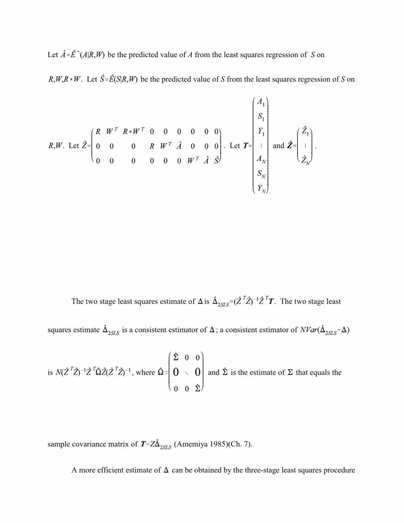
Let be the predicted value of A from the least squares regression of S on

. Let be the predicted value of S from the least squares regression of S on

. Let . Let and .

The two stage least squares estimate of is . The two stage least

squares estimate is a consistent estimator of ; a consistent estimator of

is , where and is the estimate of that equals the

sample covariance matrix of (Amemiya 1985)(Ch. 7).

A more efficient estimate of can be obtained by the three-stage least squares procedure

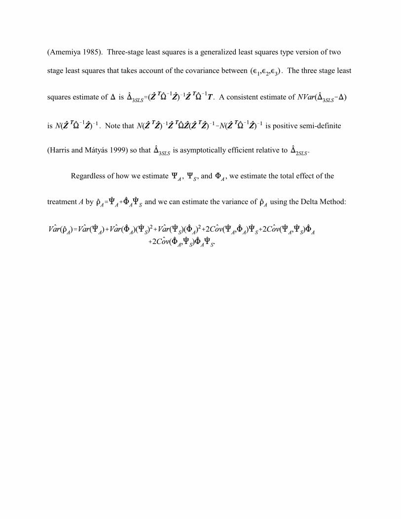
(Amemiya 1985). Three-stage least squares is a generalized least squares type version of two

stage least squares that takes account of the covariance between . The three stage least

squares estimate of is . A consistent estimate of

is . Note that is positive semi-definite

(Harris and Mátyás 1999) so that is asymptotically efficient relative to .

Regardless of how we estimate , , and , we estimate the total effect of the

treatment A by and we can estimate the variance of using the Delta Method:

Reference List

Albert, J. (2007), "Mediation analysis via potential outcome models," Statistics in Medicine, to appear.

Amemiya, T. (1985), Advanced Econometrics Cambridge: Harvard University Press.

Anderson, T., and Rubin, H. (1949), "Estimation of the parameters of coefficients of a single equation in a

simultaneous system and their asymptotic expansions," Econometrica, 41, 683-714.

Angrist, J. D., Imbens, G. W., and Rubin, D. B. (1996), "Identification of causal effects using instrumental variables

(with discussion)," Journal of the American Statistical Association, 91, 444-472.

Cox, D. R. (1972), "Regression models and life-tables (with discussion)," Journal of the Royal Statistical Society,

34, 187-220.

Cox, D. R., and Oakes, D. (1984), Analysis of Survival Data London: Chapman and Hall.

Davey, S. G., and Ebrahim, S. (2003), "'Mendelian randomization': can genetic epidemiology contribute to

understanding environmental determinants of disease?," International Journal of Epidemiology, 32, 1-22.

Dhingra, R. K., Young, E. W., Hulbert-Shearon, T. E., Leavey, S., and Port, F. K. (2001), "Type of vascular access

and mortality in US hemodialysis patients," Kidney International, 60, 1443-1451.

Feldman, H. I., Joffe, M. M., Robinson, B., Knauss, J., Cizman, B., Guo, W., Franklin-Becker, E., and Faich, G.

(2004), "Administration of parenteral iron and mortality among hemodialysis patients," Journal of the American

Society of Nephrology, 15, 1623-1632.

Harris, D., and Mátyás, L. (1999), "Introductin to the generalized method of moments," in Generalized Method of

Moments Estimation, ed. L. Mátyás, New York: Cambridge University Press.

Joffe, M. M., and Brensinger, C. (2001), "Administrative and Artificial Censoring in Censored Regression Models,"

Statistics in Medicine, 20, 2287-2304.

Joffe, M. M., and Greene, T. (2007), "A unified framework for surrogate outcomes and markers," Biometrics,

submitted.

Joffe, M. M., Small, D., and Hsu, C. Y. (2007), "Defining and estimating intervention effects for groups that will

develop an auxiliary outcome," Statistical Science, 22, to appear.

MacKinnon, D. P., Lockwood, C., West, S., and Sheets, V. (2002), "A comparison of methods to test mediation and

other intervening variable methods," Psychological Methods, 7, 83-104.

Mark, S. D., and Robins, J. M. (1993), "A method for the analysis of randomized trials with compliance information:

an application to the multiple risk factor intervention trial," Controlled Clinical Trials, 14, 79-97.

McClellan, M., and Newhouse, J. P. (1997), "The marginal cost-effectiveness of medical technology: a panel

instrumental-variables approach," Journal of Econometrics, 77, 39-64.

Newey, W. K. (1985), "Generalized method of moments specification testing," Journal of Econometrics, 29, 229-

256.

Neyman, J. (1990), "On the application of probability theory to agricultural experiments. Essay on principles.

Translated by D.M. Dabrowska and edited by T. P. Speed," Statistical Science, 5, 465-472.

Pearl, J. (1995), "Causal diagrams for empirical research," Biometrika, 83, 669-690.

----- (2000), Causality: models, reasoning, and inference Cambridge University Press.

----- (2001), "Direct and indirect effects," in Proceedings of the Seventeenth Conference on Uncertainty in Artificial

Intelligence, San Francisco: Morgan Kaufmann.

Reddan, D., Klassen, P., Frankenfield, D. L., Szczech, L., Schwab, S., Coladonato, J., Rocco, M., Lowrie, E. G., and

Owen, W. F. (2002), "National profile of practice patterns for hemodialysis vascular access in the United States,"

Journal of the American Society of Nephrology, 13, 2117-2124.

Robins, J. (1992), "Estimation of the time-dependent accelerated failure time model in the presence of confounding

factors," Biometrika, 79, 321-334.

Robins, J., and Greenland, S. (1992), "Identifiability and exchangeability for direct and indirect effects,"

Epidemiology, 3, 143-155.

Robins, J., and Rotnitzky, A. (2004), "Estimation of treatment effects in randomized trials with non-compliance and

a dichotomous outcome using structural mean models," Biometrika, 91, 763-783.

Robins, J. M. (1994), "Correcting for non-compliance in randomized trials using structural nested mean models,"

Communications in Statistics-Theory and Methods, 23, 2379-2412.

Robins, J. M., Blevins, D., Ritter, G., and Wulfsohn, M. (1992), "G-estimation of the effect of prophylaxis therapy

for pneumocystic carinii pneumonia on the survival of AIDS patients," Epidemiology, 3, 319-336.

Robins, J. M., and Greenland, S. (1994), "Adjusting for differential rates of prophylaxis therapy for PCP in high-

versus low-dose AZT treatment arms in an AIDS randomized trial," Journal of the American Statistical Association,

89, 737-749.

Robins, J. M., Rotnitzky, A., and Scharfstein, D. O. (2000), "Sensitivity analysis for selection bias and unmeasured

confounding in missing data and causal inference models," in Statistical Models in Epidemiology, eds. E. Halloran

and D. Berry, New York: Springer-Verlag.

Rosenbaum, P. R., and Rubin, D. B. (1983), "The central role of the propensity score in observational studies for

causal effects," Biometrika, 70, 41-55.

Rubin, D. B. (1974), "Estimating causal effects of treatments in randomized and nonrandomized studies," Journal of

Educational Psychology, 66, 688-701.

----- (1978), "Bayesian inference for causal effects: the role of randomization," Annals of Statistics, 6, 34-58.

Sehgal, A. R., Snow, R. J., Singer, M. E., Amini, S. A., Deoreo, P. B., Silver, M. R., and Cebul, R. D. (1998),

"Barriers to adequate delivery of dialysis," American Journal of Kidney Diseases, 31, 593-601.

Small, D. (2007), "Sensitivity Analysis for Instrumental Variables Regression With Overidentifying Restrictions,"

Journal of the American Statistical Association, in press.

Stock, J. H. (2001), "Instrumental variables in statistics and econometrics," in International Encyclopedia of the

Social and Behavioral Sciences, eds. N. J. Smelser and P. B. Baltes, New York: Elsevier Science Ltd.

Ten Have, T. R., Elliott, M. R., Joffe, M., Zanutto, E., and Datto, C. (2004), "Causal Models for Randomized

Physician Encouragement Trials in Treating Primary Care Depression," Journal of the American Statistical

Association, 99, 16-25.

Ten Have, T. R., Joffe, M. M., Lynch, K. G., Brown, G. K., Maisto, S. A., and Beck, A. T. (2007), "Causal

mediation analyses with rank preserving models," Biometrics, 63, in press.

Wolfe, R. A., Dhingra, R. K., Hulbert-Shearon, T. E., Leavey, S., and Port, F. K. (2000), "Association between

vascular access type and standardized mortality," Journal of the American Society of Nephrology, 11, 1070A.

Wolfe, R. A., Hulbert-Shearon, T. E., Ashby, V. B., Mahadevan, S., and Port, F. K. (2004), "Improvements in

dialysis patient mortality are associated with improvements in urea reduction ratio and hematocrit, 1999 to 2002,"

American Journal of Kidney Diseases, 45, 127-135.

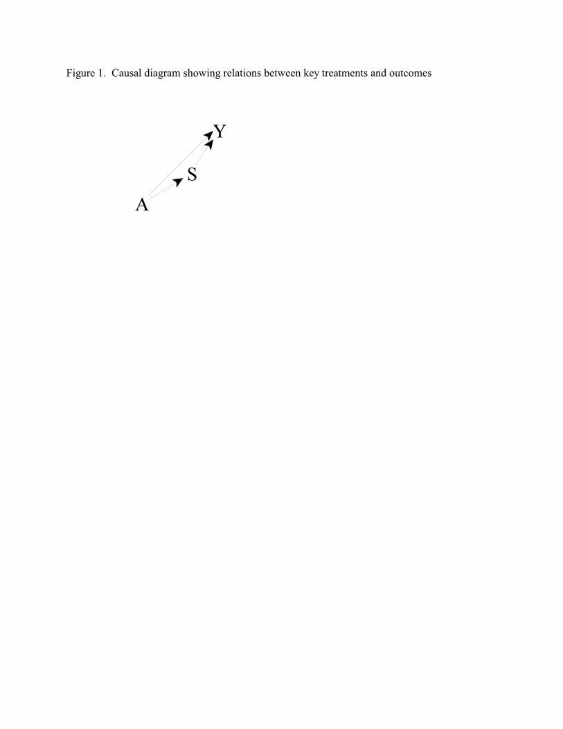
Figure 1. Causal diagram showing relations between key treatments and outcomes

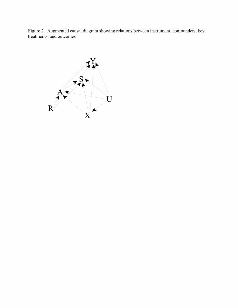
Figure 2. Augmented causal diagram showing relations between instrument, confounders, keytreatments, and outcomes

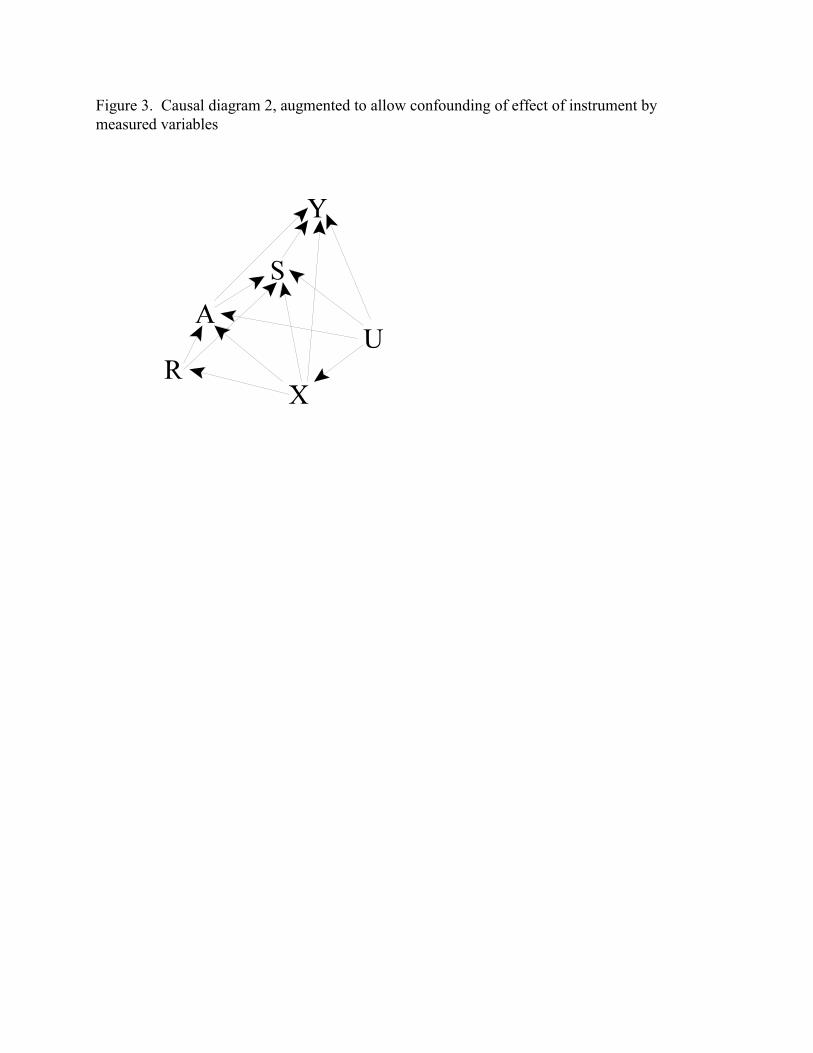
Figure 3. Causal diagram 2, augmented to allow confounding of effect of instrument bymeasured variables

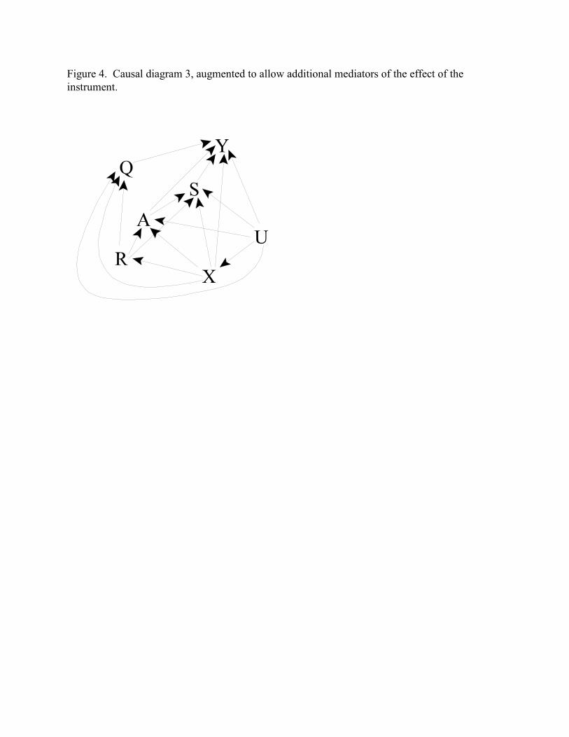
Figure 4. Causal diagram 3, augmented to allow additional mediators of the effect of theinstrument.

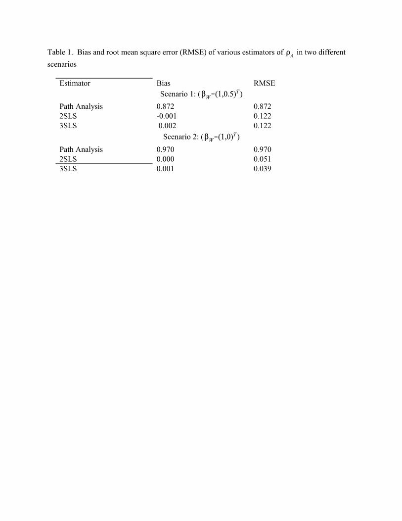
Table 1. Bias and root mean square error (RMSE) of various estimators of in two different

scenarios

Estimator Bias RMSE

Scenario 1: ( )

Path Analysis 0.872 0.8722SLS -0.001 0.1223SLS 0.002 0.122

Scenario 2: ( )

Path Analysis 0.970 0.9702SLS 0.000 0.0513SLS 0.001 0.039