1

Exploring evolutionary models with Lsd

PhD Eurolab on Simulation of Economic Evolution (SIME)University of Strasbourg, April 2004

Revised: 8 April 2004

Esben Sloth AndersenDRUID and IKE, Aalborg University, Denmark

2

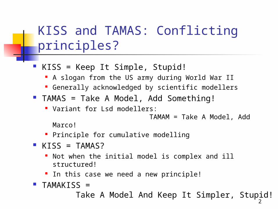
KISS and TAMAS: Conflicting principles?

KISS = Keep It Simple, Stupid! A slogan from the US army during World War II Generally acknowledged by scientific modellers

TAMAS = Take A Model, Add Something! Variant for Lsd modellers:

TAMAM = Take A Model, Add Marco! Principle for cumulative modelling

KISS = TAMAS? Not when the initial model is complex and ill structured! In this case we need a new principle!

TAMAKISS = Take A Model And Keep It Simpler, Stupid!

3

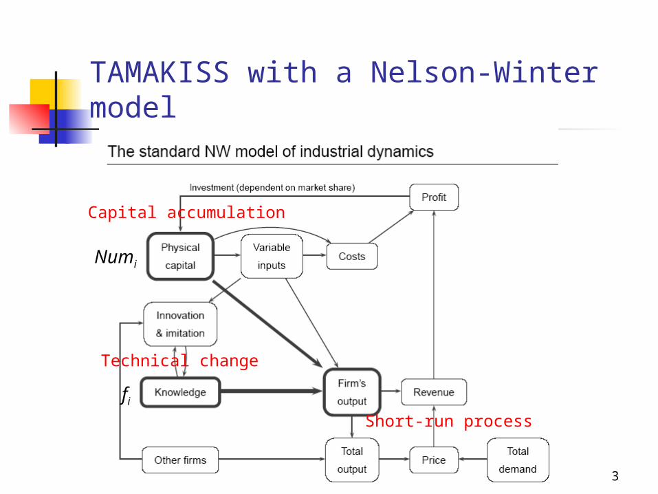
TAMAKISS with a Nelson-Winter model

Short-run process

Capital accumulation

Technical change

Numi

fi

4

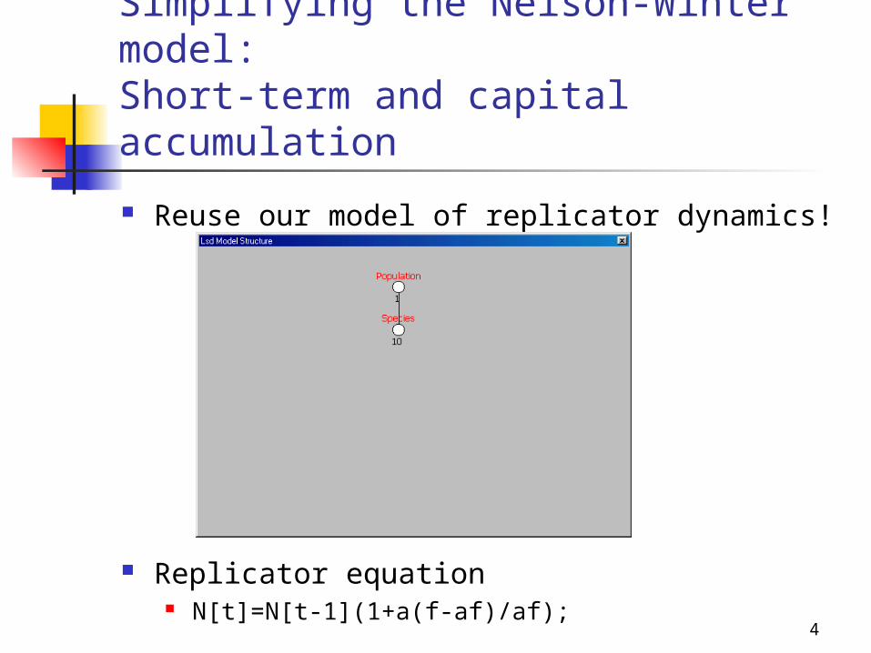
Simplifying the Nelson-Winter model:Short-term and capital accumulation

Reuse our model of replicator dynamics!

Replicator equation N[t]=N[t-1](1+a(f-af)/af);

5

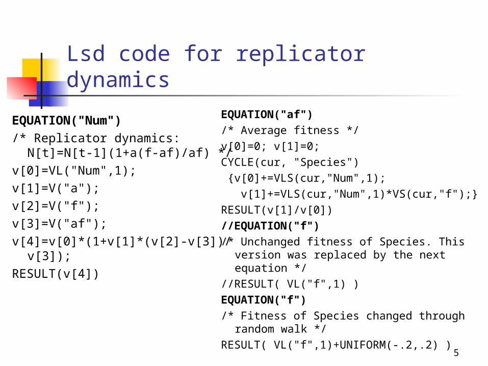
Lsd code for replicator dynamics

EQUATION("Num")/* Replicator dynamics:

N[t]=N[t-1](1+a(f-af)/af) */v[0]=VL("Num",1);v[1]=V("a");v[2]=V("f");v[3]=V("af");v[4]=v[0]*(1+v[1]*(v[2]-v[3])/v[3]);RESULT(v[4])

EQUATION("af")/* Average fitness */

v[0]=0; v[1]=0;

CYCLE(cur, "Species")

{v[0]+=VLS(cur,"Num",1);

v[1]+=VLS(cur,"Num",1)*VS(cur,"f");}RESULT(v[1]/v[0])

//EQUATION("f")

/* Unchanged fitness of Species. This version was replaced by the next equation */

//RESULT( VL("f",1) )

EQUATION("f")/* Fitness of Species changed through

random walk */

RESULT( VL("f",1)+UNIFORM(-.2,.2) )

6

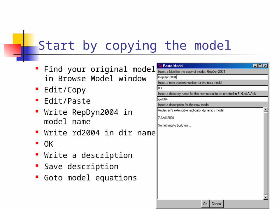
Start by copying the model

Find your original modelin Browse Model window

Edit/Copy Edit/Paste Write RepDyn2004 in

model name Write rd2004 in dir name OK Write a description Save description Goto model equations

7

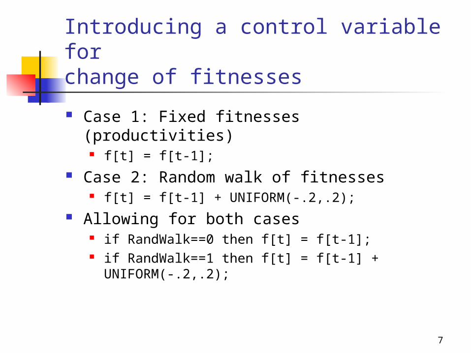
Introducing a control variable for change of fitnesses

Case 1: Fixed fitnesses (productivities) f[t] = f[t-1];

Case 2: Random walk of fitnesses f[t] = f[t-1] + UNIFORM(-.2,.2);

Allowing for both cases if RandWalk==0 then f[t] = f[t-1]; if RandWalk==1 then f[t] = f[t-1] + UNIFORM(-.2,.2);

8

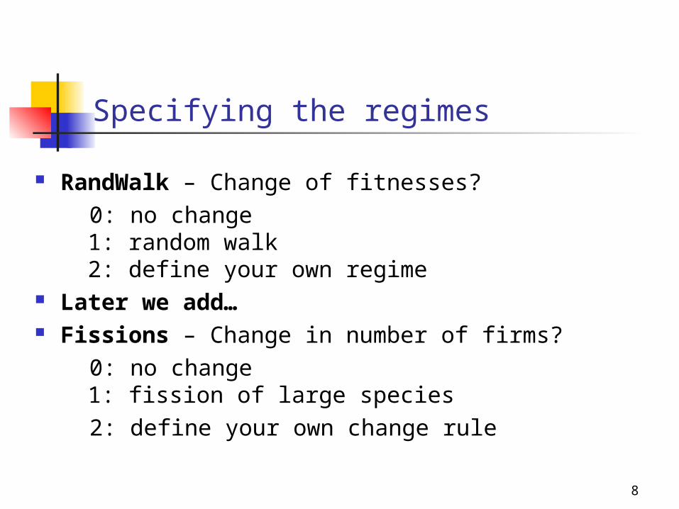
Specifying the regimes

RandWalk – Change of fitnesses?

0: no change 1: random walk 2: define your own regime

Later we add… Fissions – Change in number of firms?

0: no change 1: fission of large species

2: define your own change rule

9

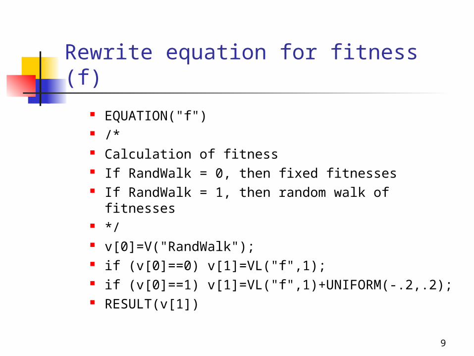
Rewrite equation for fitness (f)

EQUATION("f") /* Calculation of fitness If RandWalk = 0, then fixed fitnesses If RandWalk = 1, then random walk of fitnesses */ v[0]=V("RandWalk"); if (v[0]==0) v[1]=VL("f",1); if (v[0]==1) v[1]=VL("f",1)+UNIFORM(-.2,.2); RESULT(v[1])

10

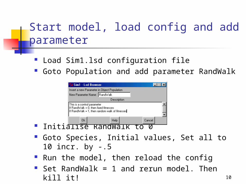
Start model, load config and add parameter

Load Sim1.lsd configuration file Goto Population and add parameter RandWalk

Initialise RandWalk to 0 Goto Species, Initial values, Set all to 10 incr. by

-.5 Run the model, then reload the config Set RandWalk = 1 and rerun model. Then kill it!

11

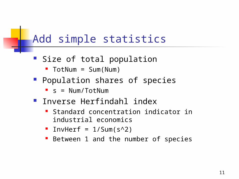
Add simple statistics

Size of total population TotNum = Sum(Num)

Population shares of species s = Num/TotNum

Inverse Herfindahl index Standard concentration indicator in industrial

economics InvHerf = 1/Sum(s^2) Between 1 and the number of species

12

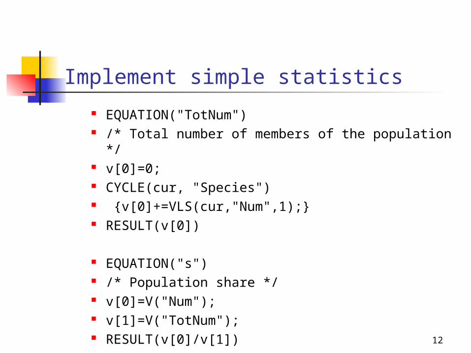
Implement simple statistics

EQUATION("TotNum") /* Total number of members of the population */ v[0]=0; CYCLE(cur, "Species") {v[0]+=VLS(cur,"Num",1);} RESULT(v[0])

EQUATION("s") /* Population share */ v[0]=V("Num"); v[1]=V("TotNum"); RESULT(v[0]/v[1])

13

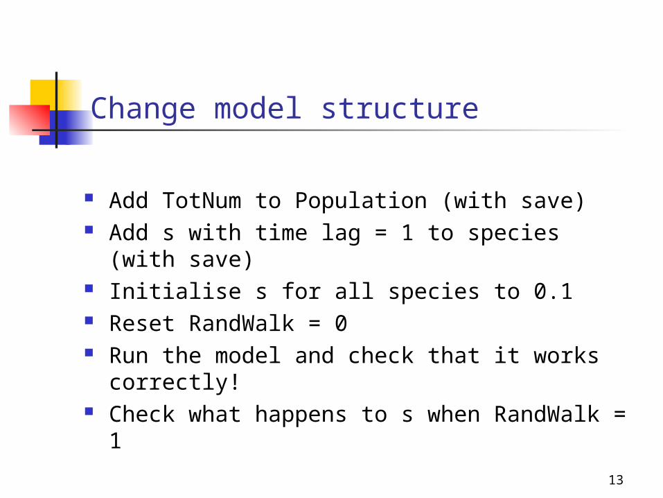
Change model structure

Add TotNum to Population (with save) Add s with time lag = 1 to species (with save) Initialise s for all species to 0.1 Reset RandWalk = 0 Run the model and check that it works

correctly! Check what happens to s when RandWalk = 1

14

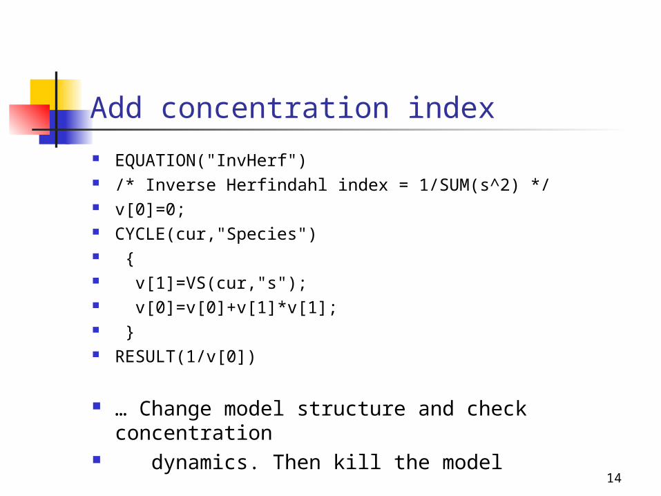
Add concentration index

EQUATION("InvHerf") /* Inverse Herfindahl index = 1/SUM(s^2) */ v[0]=0; CYCLE(cur,"Species") { v[1]=VS(cur,"s"); v[0]=v[0]+v[1]*v[1]; } RESULT(1/v[0])

… Change model structure and check concentration

dynamics. Then kill the model

15

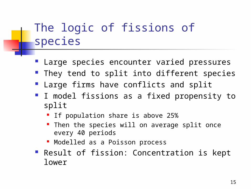
The logic of fissions of species

Large species encounter varied pressures They tend to split into different species Large firms have conflicts and split I model fissions as a fixed propensity to split

If population share is above 25% Then the species will on average split once every 40

periods Modelled as a Poisson process

Result of fission: Concentration is kept lower

16

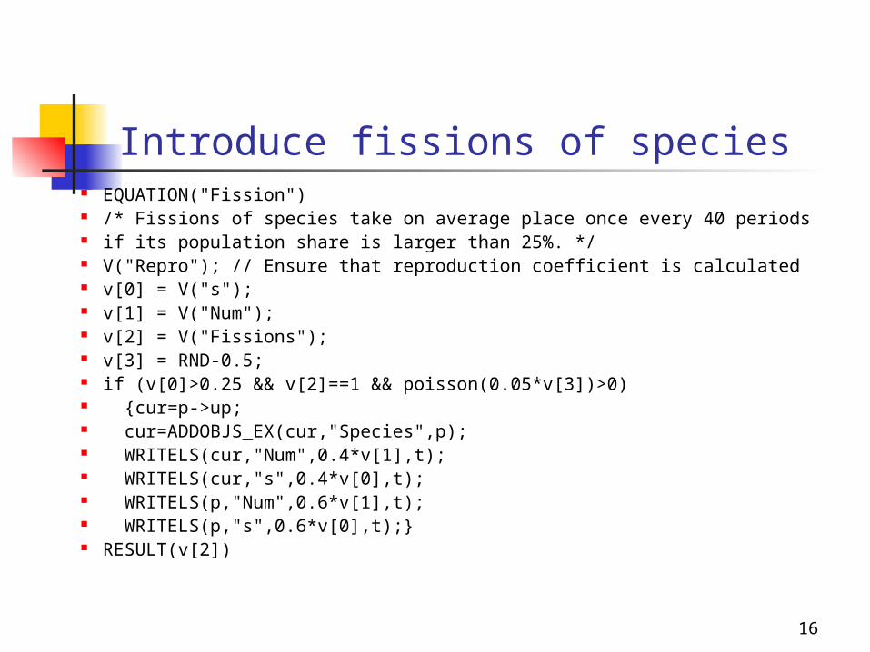
Introduce fissions of species EQUATION("Fission") /* Fissions of species take on average place once every 40 periods if its population share is larger than 25%. */ V("Repro"); // Ensure that reproduction coefficient is calculated v[0] = V("s"); v[1] = V("Num"); v[2] = V("Fissions"); v[3] = RND-0.5; if (v[0]>0.25 && v[2]==1 && poisson(0.05*v[3])>0) {cur=p->up; cur=ADDOBJS_EX(cur,"Species",p); WRITELS(cur,"Num",0.4*v[1],t); WRITELS(cur,"s",0.4*v[0],t); WRITELS(p,"Num",0.6*v[1],t); WRITELS(p,"s",0.6*v[0],t);} RESULT(v[2])

17

Change the model structure and check

Add parameter Fissions to Population Initialise Fission = 0 and RandWalk = 0 Add variable Fission to Species Run the model and check that nothing has changed Change Fission = 1, and study the results Why is there no fissions at the end of the

simulation? Change Fission = 1 and RandWalk = 1 Study the results? What happens?

Kill the model before proceeding

18

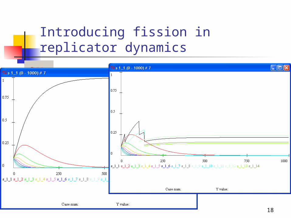
Introducing fission in replicator dynamics

19

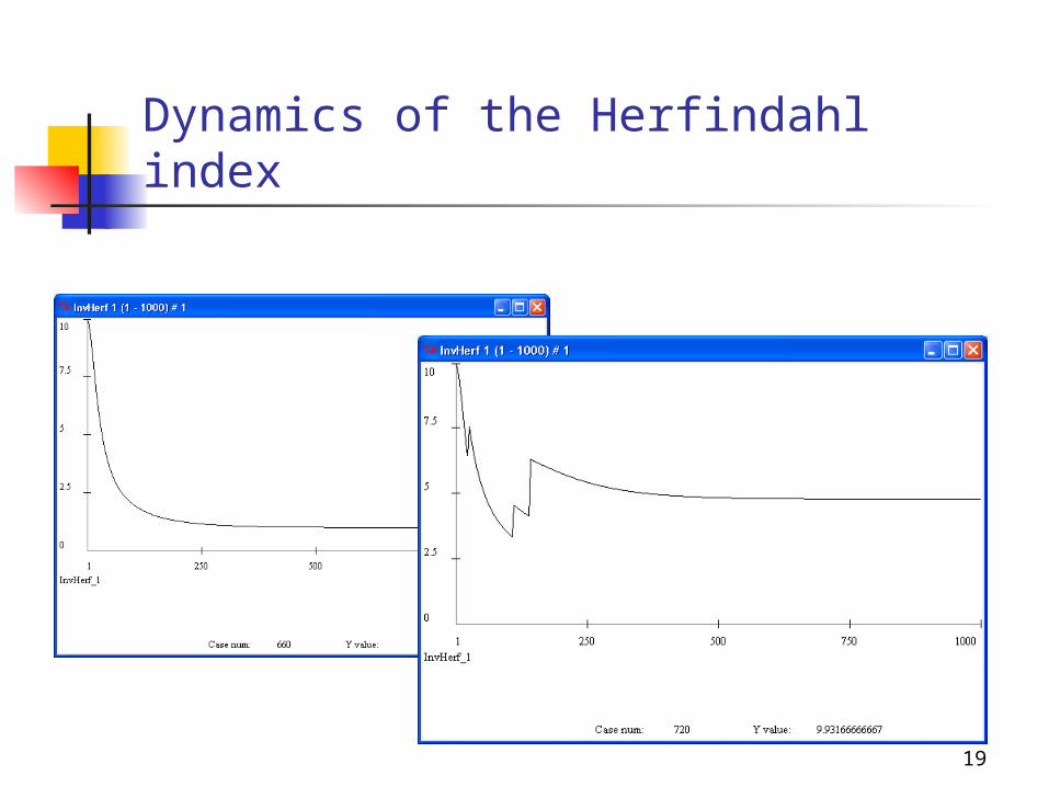
Dynamics of the Herfindahl index

20

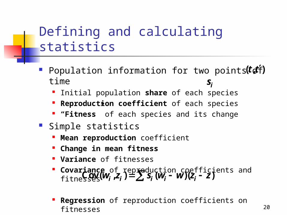
Defining and calculating statistics

Population information for two points of time Initial population share of each species Reproduction coefficient of each species “Fitness” of each species and its change

Simple statistics Mean reproduction coefficient Change in mean fitness Variance of fitnesses Covariance of reproduction coefficients and

fitnesses

Regression of reproduction coefficients on fitnesses

( , )t t

is

Cov( , ) ( )( )i i i i iw z s w w z z

21

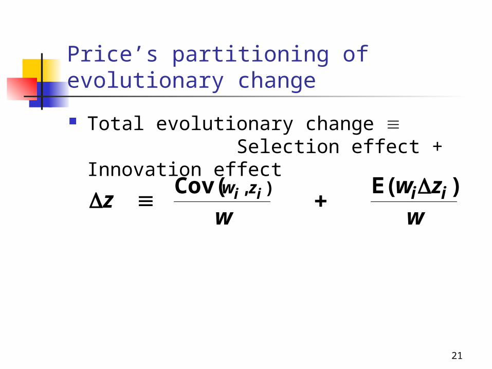
Price’s partitioning of evolutionary change

Total evolutionary change Selection effect + Innovation effect

w

zw

wz iizw ii )E(Cov( ),

22

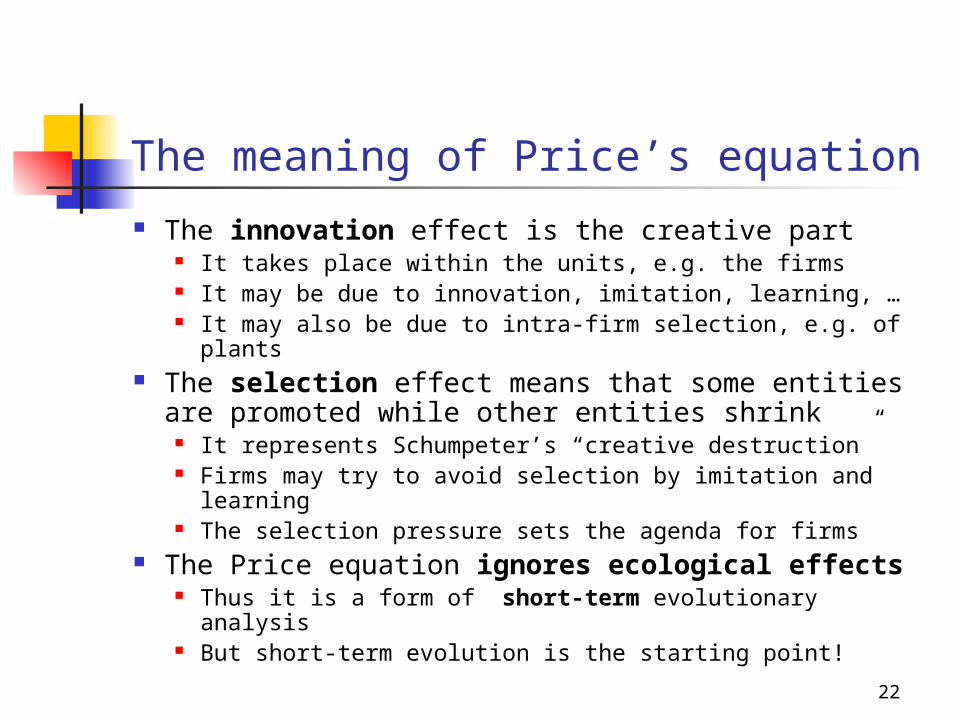
The meaning of Price’s equation

The innovation effect is the creative part It takes place within the units, e.g. the firms It may be due to innovation, imitation, learning, … It may also be due to intra-firm selection, e.g. of plants

The selection effect means that some entities are promoted while other entities shrink

It represents Schumpeter’s “creative destruction” Firms may try to avoid selection by imitation and

learning The selection pressure sets the agenda for firms

The Price equation ignores ecological effects Thus it is a form of short-term evolutionary analysis But short-term evolution is the starting point!

23

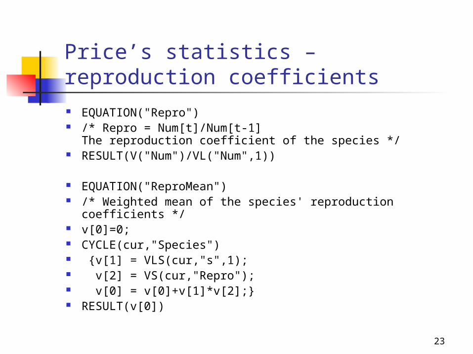
Price’s statistics – reproduction coefficients EQUATION("Repro") /* Repro = Num[t]/Num[t-1]

The reproduction coefficient of the species */ RESULT(V("Num")/VL("Num",1))

EQUATION("ReproMean") /* Weighted mean of the species' reproduction coefficients */ v[0]=0; CYCLE(cur,"Species") {v[1] = VLS(cur,"s",1); v[2] = VS(cur,"Repro"); v[0] = v[0]+v[1]*v[2];} RESULT(v[0])

24

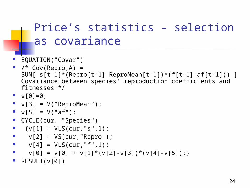
Price’s statistics – selection as covariance

EQUATION("Covar") /* Cov(Repro,A) =

SUM[ s[t-1]*(Repro[t-1]-ReproMean[t-1])*(f[t-1]-af[t-1])) ]Covariance between species' reproduction coefficients and fitnesses */

v[0]=0; v[3] = V("ReproMean"); v[5] = V("af"); CYCLE(cur, "Species") {v[1] = VLS(cur,"s",1); v[2] = VS(cur,"Repro"); v[4] = VLS(cur,"f",1); v[0] = v[0] + v[1]*(v[2]-v[3])*(v[4]-v[5]);} RESULT(v[0])

25

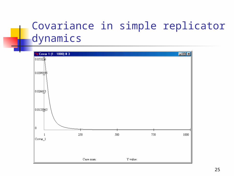
Covariance in simple replicator dynamics

26

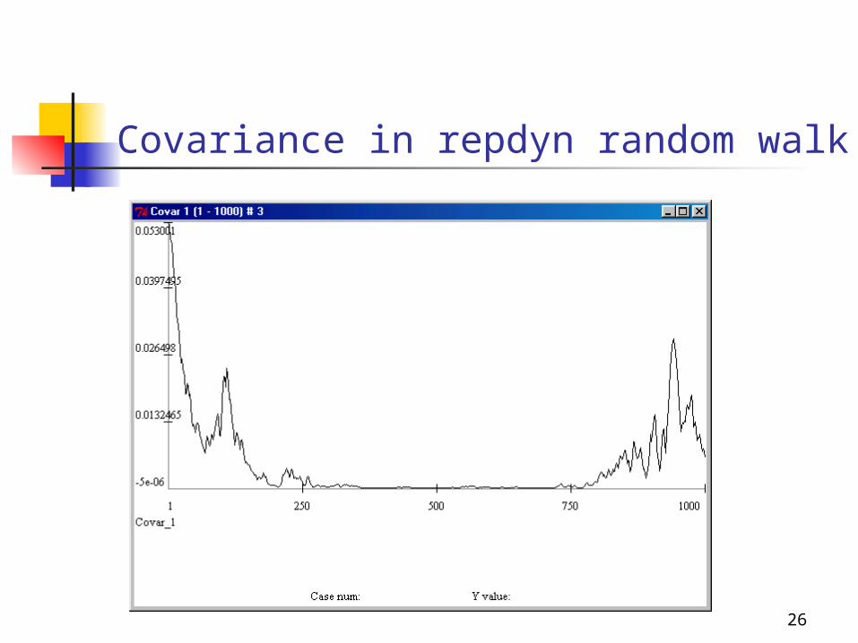
Covariance in repdyn random walk

27

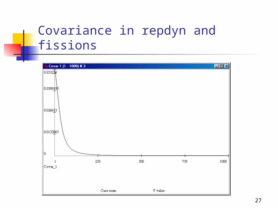
Covariance in repdyn and fissions

28

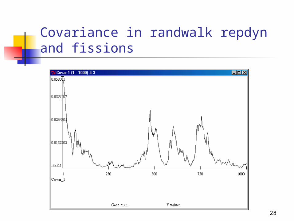
Covariance in randwalk repdyn and fissions

29

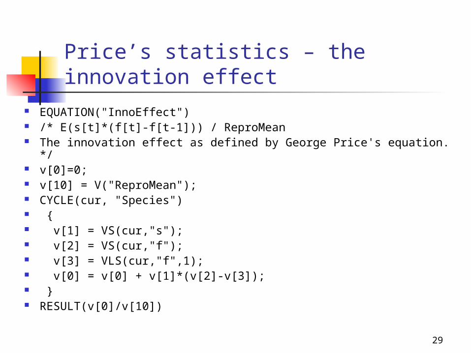
Price’s statistics – the innovation effect

EQUATION("InnoEffect") /* E(s[t]*(f[t]-f[t-1])) / ReproMean The innovation effect as defined by George Price's equation. */ v[0]=0; v[10] = V("ReproMean"); CYCLE(cur, "Species") { v[1] = VS(cur,"s"); v[2] = VS(cur,"f"); v[3] = VLS(cur,"f",1); v[0] = v[0] + v[1]*(v[2]-v[3]); } RESULT(v[0]/v[10])

30

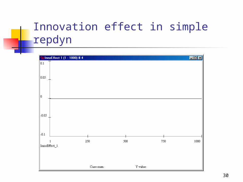
Innovation effect in simple repdyn

31

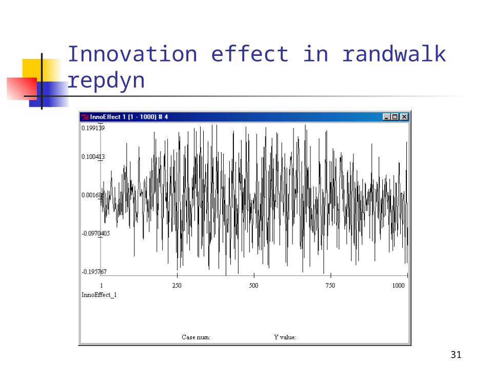
Innovation effect in randwalk repdyn