TECHNICAL NOTE 1

Evaluating array resolutionJørgen Grythe, Norsonic AS, Oslo, Norway

Abstract—Both the size and shape of an array determinethe resolution of which we can distinguish different signalsand sources. By inspecting the beampattern of the array, wecan analyse the resolution for different array configurations anddifferent input frequencies. The resolution however is both aproduct of mainlobe width and side lobe level.

Index Terms—Beampattern, array resolution, half powerbeamwidth, maximum side lobe level, acoustic eraser

INTRODUCTION

THE resolution of a beamformer represents its capabilityto separate two incoming plane waves arriving at different

angles accurately, thus assessing how well sources can bedistinguished. The choice of array geometry and sensorweights all affect this capability. Often resolution is definedaccording to measuring the width of the array beampattern’smainlobe. Mainlobe width decides how accurately the arrayis able to determine a wave’s direction of propagation, andthis width is inversely related to array geometry and size. Inaddition to mainlobe width, also the maximum side lobe levelshould be taken into consideration when assessing the overallperformance of an array. Whereas the overall size generallydetermines the width of the mainlobe, the number, positionand weighting of microphones will generally determine sidelobe level.

I. MAINLOBE WIDTH

A. Rayleigh criterion

One classical definition of resolution is the Rayleigh crite-rion, which states that two incoherent plane waves, propa-gating in two slightly different directions, are resolved if themainlobe peak of the beampattern for one wave, falls on thefirst zero of the beampattern of the other. Or said in otherwords, the mainlobe width is given as the angular distancebetween the mainlobe peak and the first zero (or half themainlobe width).

Looking at Fig. 1 we can see the beampattern of the arrayfor two incoming plane waves of equal frequency and equalstrength, but at different angles. The angles are chosen sothat for that specific frequency, the mainlobe peak of thebeampattern of the array from one wave, falls on the first zeroof the beampattern of the array for the other. The resolutionin this case is given as the angle between the two incomingwaves, or in Fig. 1 approximately 10 degrees.

Revised August 27, 2015J. Grythe is currently working as Application Manager at Norsonic, Lier,

Norway (email: jorgen.grythe@norsonic.com)

θ

-50 -40 -30 -20 -10 0 10 20 30 40 50

dB

-60

-50

-40

-30

-20

-10

0Rayleigh criterion for resolution

Fig. 1. Rayleigh criterion for resolution of two waves of equal strength andequal frequency. The mainlobe peak of the beampattern for one wave fallson the first zero of the beampattern of the other.

B. Half power beamwidth (HPBW)

The width of the mainlobe measured between the pointswhere the beampattern power has been halfed, the half powerbeamwidth (HPBW), is another useful measure of mainlobewidth. HPBW is the distance between the angles for whichthe array yields -3 dB attenuation, that is, the power from thepeak of the beampattern has dropped 3 dB as seen in Fig2. The distance between the angles defines the two sidedopening angle of the array. The beampattern is dependenton array configuration, and the two sided opening angle willbe frequency dependent, and can theoretically be used todetermine the resolution of the array for different frequencies.

θ

-50 -40 -30 -20 -10 0 10 20 30 40 50

dB

-60

-50

-40

-30

-20

-10

-30

Half Power Beamwidth (HPBW)

Fig. 2. Two-sided opening angle for half power beamwidth.

Rather than plotting the beampattern for a single frequencyonly, we can also look at the array response for angles

TECHNICAL NOTE 2

50

Beampattern with uniform weighting

0θ-50

15

10kHz

5

-40

-20

0

0

dB

kHz

2 4 6 8 10 12 14

θ

-50

0

50

-40dB-30dB-20dB-10dB0

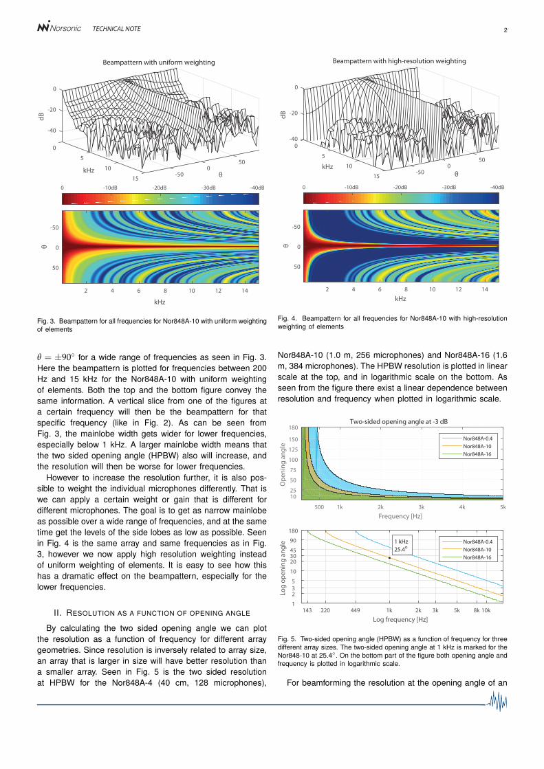
Fig. 3. Beampattern for all frequencies for Nor848A-10 with uniform weightingof elements

θ = ±90◦ for a wide range of frequencies as seen in Fig. 3.Here the beampattern is plotted for frequencies between 200Hz and 15 kHz for the Nor848A-10 with uniform weightingof elements. Both the top and the bottom figure convey thesame information. A vertical slice from one of the figures ata certain frequency will then be the beampattern for thatspecific frequency (like in Fig. 2). As can be seen fromFig. 3, the mainlobe width gets wider for lower frequencies,especially below 1 kHz. A larger mainlobe width means thatthe two sided opening angle (HPBW) also will increase, andthe resolution will then be worse for lower frequencies.

However to increase the resolution further, it is also pos-sible to weight the individual microphones differently. That iswe can apply a certain weight or gain that is different fordifferent microphones. The goal is to get as narrow mainlobeas possible over a wide range of frequencies, and at the sametime get the levels of the side lobes as low as possible. Seenin Fig. 4 is the same array and same frequencies as in Fig.3, however we now apply high resolution weighting insteadof uniform weighting of elements. It is easy to see how thishas a dramatic effect on the beampattern, especially for thelower frequencies.

II. RESOLUTION AS A FUNCTION OF OPENING ANGLE

By calculating the two sided opening angle we can plotthe resolution as a function of frequency for different arraygeometries. Since resolution is inversely related to array size,an array that is larger in size will have better resolution thana smaller array. Seen in Fig. 5 is the two sided resolutionat HPBW for the Nor848A-4 (40 cm, 128 microphones),

50

Beampattern with high-resolution weighting

0

θ-5015

10kHz

5

-40

0

-20

0

dB

kHz

2 4 6 8 10 12 14θ

-50

0

50

-40dB-30dB-20dB-10dB0

Fig. 4. Beampattern for all frequencies for Nor848A-10 with high-resolutionweighting of elements

Nor848A-10 (1.0 m, 256 microphones) and Nor848A-16 (1.6m, 384 microphones). The HPBW resolution is plotted in linearscale at the top, and in logarithmic scale on the bottom. Asseen from the figure there exist a linear dependence betweenresolution and frequency when plotted in logarithmic scale.

Two-sided opening angle at -3 dB

Frequency [Hz]

500 1k 2k 3k 4k 5k

Op

en

ing

an

gle

10 25

50

75

100

125

150

180

Nor848A-0.4

Nor848A-10

Nor848A-16

Log frequency [Hz]

143 220 449 1k 2k 3k 5k 8k 10k

Lo

g o

pe

nin

g a

ng

le

1

2 3

5

10

20 30 45

90

180

Nor848A-0.4

Nor848A-10

Nor848A-16

1 kHz

25.4o

Fig. 5. Two-sided opening angle (HPBW) as a function of frequency for threedifferent array sizes. The two-sided opening angle at 1 kHz is marked for theNor848-10 at 25.4◦. On the bottom part of the figure both opening angle andfrequency is plotted in logarithmic scale.

For beamforming the resolution at the opening angle of an

TECHNICAL NOTE 3

array is determined by the array size D and the frequency f ,or wavelength λ of the received signal

HPBW ∝λ

D=

cf · D

(1)

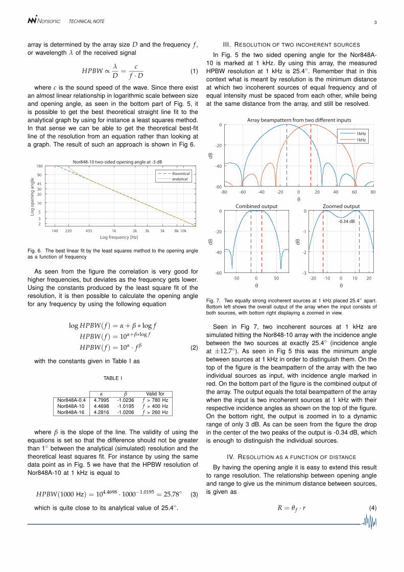
where c is the sound speed of the wave. Since there existan almost linear relationship in logarithmic scale between sizeand opening angle, as seen in the bottom part of Fig. 5, itis possible to get the best theoretical straight line fit to theanalytical graph by using for instance a least squares method.In that sense we can be able to get the theoretical best-fitline of the resolution from an equation rather than looking ata graph. The result of such an approach is shown in Fig 6.

Log frequency [Hz]

140 220 435 1k 2k 3k 5k 8k 10k

Lo

g o

pe

nin

g a

ng

le

2

3

5

10

20

30

45

90

180Nor848-10 two-sided opening angle at -3 dB

theoretical

analytical

Fig. 6. The best linear fit by the least squares method to the opening angleas a function of frequency

As seen from the figure the correlation is very good forhigher frequencies, but deviates as the frequency gets lower.Using the constants produced by the least square fit of theresolution, it is then possible to calculate the opening anglefor any frequency by using the following equation

log HPBW( f ) = α + β ∗ log f

HPBW( f ) = 10α+β∗log f

HPBW( f ) = 10α · f β (2)

with the constants given in Table I as

TABLE I

α β Valid forNor848A-0.4 4.7995 -1.0236 f > 780 HzNor848A-10 4.4698 -1.0195 f > 400 HzNor848A-16 4.2816 -1.0206 f > 260 Hz

where β is the slope of the line. The validity of using theequations is set so that the difference should not be greaterthan 1◦ between the analytical (simulated) resolution and thetheoretical least squares fit. For instance by using the samedata point as in Fig. 5 we have that the HPBW resolution ofNor848A-10 at 1 kHz is equal to

HPBW(1000 Hz) = 104.4698 · 1000−1.0195 = 25.78◦ (3)

which is quite close to its analytical value of 25.4◦.

III. RESOLUTION OF TWO INCOHERENT SOURCES

In Fig. 5 the two sided opening angle for the Nor848A-10 is marked at 1 kHz. By using this array, the measuredHPBW resolution at 1 kHz is 25.4◦. Remember that in thiscontext what is meant by resolution is the minimum distanceat which two incoherent sources of equal frequency and ofequal intensity must be spaced from each other, while beingat the same distance from the array, and still be resolved.

θ

-80 -60 -40 -20 0 20 40 60 80

dB

-60

-40

-20

0Array beampattern from two di!erent inputs

1kHz

1kHz

θ

-50 0 50

dB

-60

-40

-20

0Combined output

θ

-20 -10 0 10 20

dB

-3

-2

-1

0Zoomed output

-0.34 dB

Fig. 7. Two equally strong incoherent sources at 1 kHz placed 25.4◦ apart.Bottom left shows the overall output of the array when the input consists ofboth sources, with bottom right displaying a zoomed in view.

Seen in Fig 7, two incoherent sources at 1 kHz aresimulated hitting the Nor848-10 array with the incidence anglebetween the two sources at exactly 25.4◦ (incidence angleat ±12.7◦). As seen in Fig 5 this was the minimum anglebetween sources at 1 kHz in order to distinguish them. On thetop of the figure is the beampattern of the array with the twoindividual sources as input, with incidence angle marked inred. On the bottom part of the figure is the combined output ofthe array. The output equals the total beampattern of the arraywhen the input is two incoherent sources at 1 kHz with theirrespective incidence angles as shown on the top of the figure.On the bottom right, the output is zoomed in to a dynamicrange of only 3 dB. As can be seen from the figure the dropin the center of the two peaks of the output is -0.34 dB, whichis enough to distinguish the individual sources.

IV. RESOLUTION AS A FUNCTION OF DISTANCE

By having the opening angle it is easy to extend this resultto range resolution. The relationship between opening angleand range to give us the minimum distance between sources,is given as

R = θ f · r (4)

TECHNICAL NOTE 4

where R is the minimum distance between sources, θ f isthe two sided opening angle in radians at a given frequencyf , and r is the distance from the array to the source. Or byusing the results in (2) directly, the minimum distance betweensources can also be calculated as

R =r · 10α · f β · π

180(5)

where r is the measurement distance, f the measurementfrequency, and the constants α and β are found in Table I.

Distance [m]

2 4 6 8 10 12 14

Re

solu

tio

n [

m]

0

2

4

6

8

10

12

14Frequency: 1000 Hz

NOR848A-4

NOR848A-10

NOR848A-16

4.43 m

Fig. 8. Resolution as a function of distance for three different array sizes at1 kHz

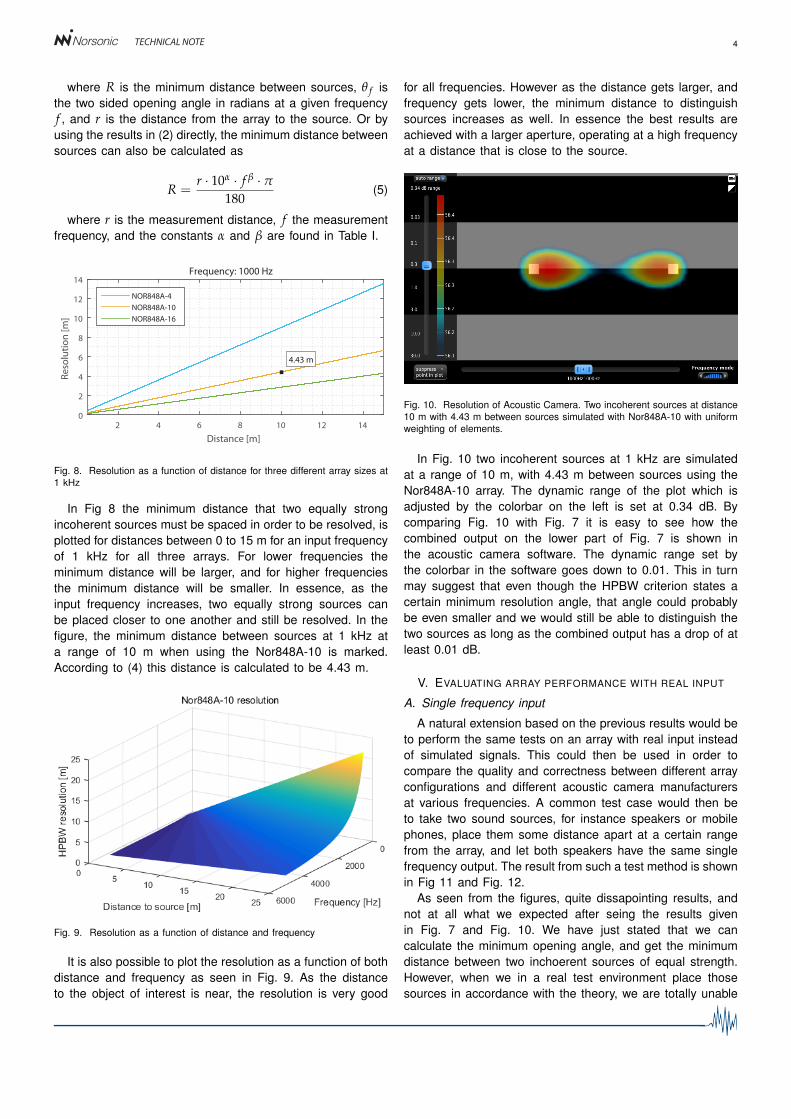
In Fig 8 the minimum distance that two equally strongincoherent sources must be spaced in order to be resolved, isplotted for distances between 0 to 15 m for an input frequencyof 1 kHz for all three arrays. For lower frequencies theminimum distance will be larger, and for higher frequenciesthe minimum distance will be smaller. In essence, as theinput frequency increases, two equally strong sources canbe placed closer to one another and still be resolved. In thefigure, the minimum distance between sources at 1 kHz ata range of 10 m when using the Nor848A-10 is marked.According to (4) this distance is calculated to be 4.43 m.

Fig. 9. Resolution as a function of distance and frequency

It is also possible to plot the resolution as a function of bothdistance and frequency as seen in Fig. 9. As the distanceto the object of interest is near, the resolution is very good

for all frequencies. However as the distance gets larger, andfrequency gets lower, the minimum distance to distinguishsources increases as well. In essence the best results areachieved with a larger aperture, operating at a high frequencyat a distance that is close to the source.

Fig. 10. Resolution of Acoustic Camera. Two incoherent sources at distance10 m with 4.43 m between sources simulated with Nor848A-10 with uniformweighting of elements.

In Fig. 10 two incoherent sources at 1 kHz are simulatedat a range of 10 m, with 4.43 m between sources using theNor848A-10 array. The dynamic range of the plot which isadjusted by the colorbar on the left is set at 0.34 dB. Bycomparing Fig. 10 with Fig. 7 it is easy to see how thecombined output on the lower part of Fig. 7 is shown inthe acoustic camera software. The dynamic range set bythe colorbar in the software goes down to 0.01. This in turnmay suggest that even though the HPBW criterion states acertain minimum resolution angle, that angle could probablybe even smaller and we would still be able to distinguish thetwo sources as long as the combined output has a drop of atleast 0.01 dB.

V. EVALUATING ARRAY PERFORMANCE WITH REAL INPUT

A. Single frequency input

A natural extension based on the previous results would beto perform the same tests on an array with real input insteadof simulated signals. This could then be used in order tocompare the quality and correctness between different arrayconfigurations and different acoustic camera manufacturersat various frequencies. A common test case would then beto take two sound sources, for instance speakers or mobilephones, place them some distance apart at a certain rangefrom the array, and let both speakers have the same singlefrequency output. The result from such a test method is shownin Fig 11 and Fig. 12.

As seen from the figures, quite dissapointing results, andnot at all what we expected after seing the results givenin Fig. 7 and Fig. 10. We have just stated that we cancalculate the minimum opening angle, and get the minimumdistance between two inchoerent sources of equal strength.However, when we in a real test environment place thosesources in accordance with the theory, we are totally unable

TECHNICAL NOTE 5

θ

-80 -60 -40 -20 0 20 40 60 80

dB

-60

-40

-20

0Array beampattern from two di!erent inputs

1kHz

1kHz

θ

-50 0 50

dB

-60

-40

-20

0Combined output

θ

-20 -10 0 10 20

dB

-6

-3

-1

0Zoomed output

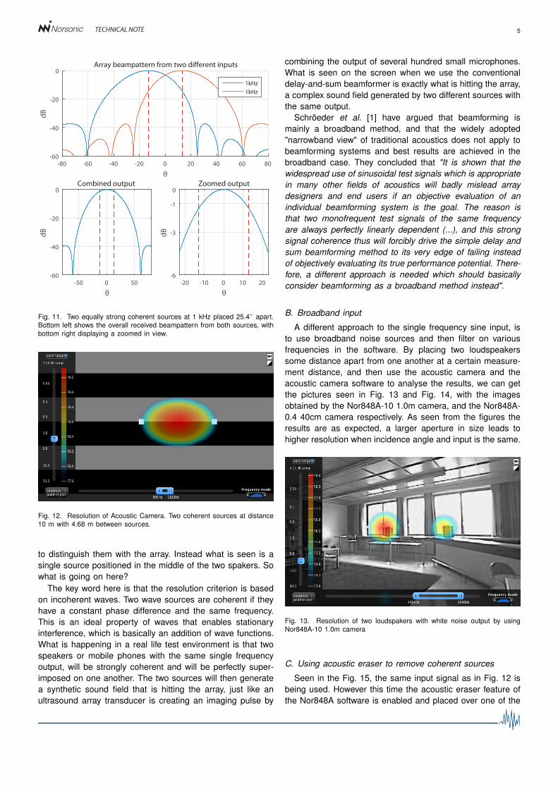
Fig. 11. Two equally strong coherent sources at 1 kHz placed 25.4◦ apart.Bottom left shows the overall received beampattern from both sources, withbottom right displaying a zoomed in view.

Fig. 12. Resolution of Acoustic Camera. Two coherent sources at distance10 m with 4.68 m between sources.

to distinguish them with the array. Instead what is seen is asingle source positioned in the middle of the two spakers. Sowhat is going on here?

The key word here is that the resolution criterion is basedon incoherent waves. Two wave sources are coherent if theyhave a constant phase difference and the same frequency.This is an ideal property of waves that enables stationaryinterference, which is basically an addition of wave functions.What is happening in a real life test environment is that twospeakers or mobile phones with the same single frequencyoutput, will be strongly coherent and will be perfectly super-imposed on one another. The two sources will then generatea synthetic sound field that is hitting the array, just like anultrasound array transducer is creating an imaging pulse by

combining the output of several hundred small microphones.What is seen on the screen when we use the conventionaldelay-and-sum beamformer is exactly what is hitting the array,a complex sound field generated by two different sources withthe same output.

Schröeder et al. [1] have argued that beamforming ismainly a broadband method, and that the widely adopted"narrowband view" of traditional acoustics does not apply tobeamforming systems and best results are achieved in thebroadband case. They concluded that "It is shown that thewidespread use of sinusoidal test signals which is appropriatein many other fields of acoustics will badly mislead arraydesigners and end users if an objective evaluation of anindividual beamforming system is the goal. The reason isthat two monofrequent test signals of the same frequencyare always perfectly linearly dependent (...), and this strongsignal coherence thus will forcibly drive the simple delay andsum beamforming method to its very edge of failing insteadof objectively evaluating its true performance potential. There-fore, a different approach is needed which should basicallyconsider beamforming as a broadband method instead".

B. Broadband input

A different approach to the single frequency sine input, isto use broadband noise sources and then filter on variousfrequencies in the software. By placing two loudspeakerssome distance apart from one another at a certain measure-ment distance, and then use the acoustic camera and theacoustic camera software to analyse the results, we can getthe pictures seen in Fig. 13 and Fig. 14, with the imagesobtained by the Nor848A-10 1.0m camera, and the Nor848A-0.4 40cm camera respectively. As seen from the figures theresults are as expected, a larger aperture in size leads tohigher resolution when incidence angle and input is the same.

Fig. 13. Resolution of two loudspakers with white noise output by usingNor848A-10 1.0m camera

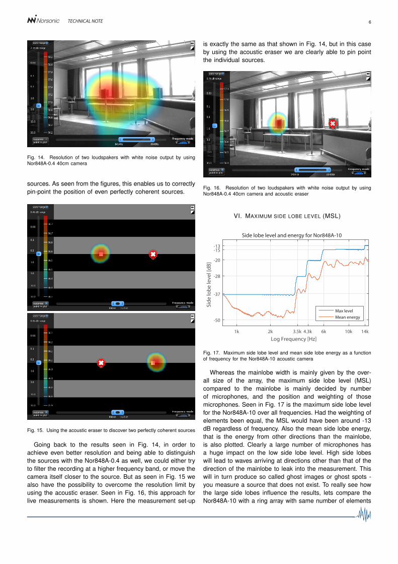
C. Using acoustic eraser to remove coherent sources

Seen in the Fig. 15, the same input signal as in Fig. 12 isbeing used. However this time the acoustic eraser feature ofthe Nor848A software is enabled and placed over one of the

TECHNICAL NOTE 6

Fig. 14. Resolution of two loudspakers with white noise output by usingNor848A-0.4 40cm camera

sources. As seen from the figures, this enables us to correctlypin-point the position of even perfectly coherent sources.

Fig. 15. Using the acoustic eraser to discover two perfectly coherent sources

Going back to the results seen in Fig. 14, in order toachieve even better resolution and being able to distinguishthe sources with the Nor848A-0.4 as well, we could either tryto filter the recording at a higher frequency band, or move thecamera itself closer to the source. But as seen in Fig. 15 wealso have the possibility to overcome the resolution limit byusing the acoustic eraser. Seen in Fig. 16, this approach forlive measurements is shown. Here the measurement set-up

is exactly the same as that shown in Fig. 14, but in this caseby using the acoustic eraser we are clearly able to pin pointthe individual sources.

Fig. 16. Resolution of two loudspakers with white noise output by usingNor848A-0.4 40cm camera and acoustic eraser

VI. MAXIMUM SIDE LOBE LEVEL (MSL)

Log Frequency [Hz]

1k 2k 3.5k 4.3k 6k 10k 14k

Sid

e lo

be

lev

el [

dB

]

-50

-37

-28

-20

-15-13

Side lobe level and energy for Nor848A-10

Max level

Mean energy

Fig. 17. Maximum side lobe level and mean side lobe energy as a functionof frequency for the Nor848A-10 acoustic camera

Whereas the mainlobe width is mainly given by the over-all size of the array, the maximum side lobe level (MSL)compared to the mainlobe is mainly decided by numberof microphones, and the position and weighting of thosemicrophones. Seen in Fig. 17 is the maximum side lobe levelfor the Nor848A-10 over all frequencies. Had the weighting ofelements been equal, the MSL would have been around -13dB regardless of frequency. Also the mean side lobe energy,that is the energy from other directions than the mainlobe,is also plotted. Clearly a large number of microphones hasa huge impact on the low side lobe level. High side lobeswill lead to waves arriving at directions other than that of thedirection of the mainlobe to leak into the measurement. Thiswill in turn produce so called ghost images or ghost spots -you measure a source that does not exist. To really see howthe large side lobes influence the results, lets compare theNor848A-10 with a ring array with same number of elements

TECHNICAL NOTE 7

and same size. The ring array then has 256 microphonesplaced evenly in a circle with diameter of 1.0 m as seen inFig 18.

Nor848A-10 Ring array

Fig. 18. Array geometry of Nor848A-10 and ring array with same number ofelements and same diameter.

We can now calculate and analyze the beampattern atfrequency f = 3 kHz for the two different arrays as seenin Fig. 19, with a zoomed version of the same beampatternseen in Fig. 20.

Angle (deg)

-80 -60 -40 -20 0 20 40 60 80

Att

en

ua

tio

n (

dB

)

-50

-40

-30

-20

-10

-30

Ring array

Nor848A-10

Fig. 19. Beampattern of Nor848A-10 and ring array with same number ofelements and same diameter simulated at 3 kHz.

Angle (deg)

-20 -10 0 10 20

Att

en

ua

tio

n (

dB

)

-15

-10

-6

-3

0

Ring array

Nor848A-10

Fig. 20. Zoomed in view of beampattern at 3 kHz. The half power beamwidthof the ring array is more narrow than for the Nor848A-10.

Now judging from the beampattern alone, and according

to the HPBW standard, the ring array should have the bestresolution as the opening angle at -3 dB is more narrow thanthe same opening angle for the Nor848A-10. To see how thiswill influence an acoustic image, we can simulate the arrayoutput from the two different arrays for a custom test signal ofour choice. Seen in Fig. 21 is just such an approach wherethe two different arrays are scanning over all incidence angleslooking for nine point sources of equal strength and equalfrequency f = 3 kHz. The dynamic range of the picture hasbeen set equal for both images at 4 dB. As we can see fromFig. 21, both arrays are able to pin point the location of thedifferent point sources, however the accuracy is better for thering array at the same dynamic range. This is logical sincethe mainlobe of the beampattern at that frequency is morenarrow for the ring array than for Nor848A-10.

Nor848A-10 Ring array

Fig. 21. Simulation of array output for Nor848A-10 and ring array with ninepoint sources with frequency 3 kHz and equal power as input. Dynamic rangein the image is set to 4 dB.

Now however, let’s change the dynamic range of the imageto 8 dB instead of 4 dB. By doing this we get the imagesshown in Fig. 22

Nor848A-10 Ring array

Fig. 22. Simulation of array output for Nor848A-10 and ring array with ninepoint sources with frequency 3 kHz and equal power as input. Dynamic rangein the image is set to 8 dB.

Now we are seeing the effects of the high side-lobe levelsmuch more clearly for the ring array than for Nor848A-10.The strength of the first side-lobe of the ring array was onlyaround 8 dB lower than the mainlobe, which means that whendisplaying the image with dynamic range of 8 dB, power fromside-lobes are leaking in to the image, and smearing theresolution. This is the so called ghost-spot effect.

TECHNICAL NOTE 8

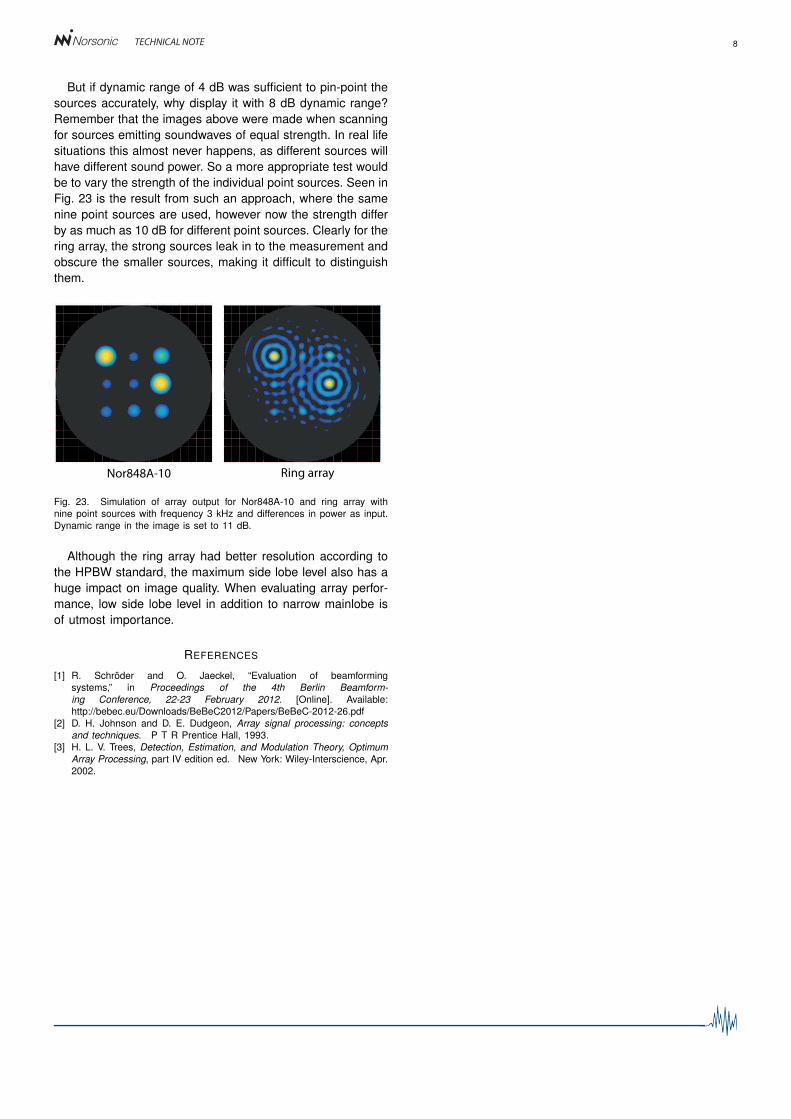
But if dynamic range of 4 dB was sufficient to pin-point thesources accurately, why display it with 8 dB dynamic range?Remember that the images above were made when scanningfor sources emitting soundwaves of equal strength. In real lifesituations this almost never happens, as different sources willhave different sound power. So a more appropriate test wouldbe to vary the strength of the individual point sources. Seen inFig. 23 is the result from such an approach, where the samenine point sources are used, however now the strength differby as much as 10 dB for different point sources. Clearly for thering array, the strong sources leak in to the measurement andobscure the smaller sources, making it difficult to distinguishthem.

Nor848A-10 Ring array

Fig. 23. Simulation of array output for Nor848A-10 and ring array withnine point sources with frequency 3 kHz and differences in power as input.Dynamic range in the image is set to 11 dB.

Although the ring array had better resolution according tothe HPBW standard, the maximum side lobe level also has ahuge impact on image quality. When evaluating array perfor-mance, low side lobe level in addition to narrow mainlobe isof utmost importance.

REFERENCES

[1] R. Schröder and O. Jaeckel, “Evaluation of beamformingsystems,” in Proceedings of the 4th Berlin Beamform-ing Conference, 22-23 February 2012. [Online]. Available:http://bebec.eu/Downloads/BeBeC2012/Papers/BeBeC-2012-26.pdf

[2] D. H. Johnson and D. E. Dudgeon, Array signal processing: conceptsand techniques. P T R Prentice Hall, 1993.

[3] H. L. V. Trees, Detection, Estimation, and Modulation Theory, OptimumArray Processing, part IV edition ed. New York: Wiley-Interscience, Apr.2002.