1

Estimation of Panel Vector Autoregression in Stata: a Package of Programs

Michael R.M. Abrigo and Inessa Love

(February 2015)

Abstract. Panel vector autoregression (VAR) models have been increasingly used in applied research.

While programs specifically designed to estimate time-series VAR models are often included as standard

features in most statistical packages, panel VAR model estimation and inference are often implemented

with general-use routines that require some programming dexterity. In this paper, we briefly discuss

model selection, estimation and inference of panel VAR models in a generalized method of moments

(GMM) framework, and present a set of Stata programs to conveniently execute them. We illustrate the

pvar package of programs by using standard Stata datasets.

1

Estimation of panel vector autoregression in Stata: A package of programs

Michael R.M. Abrigo*1 and Inessa Love2

(February 2015)

1. Introduction

Time-series vector autoregression (VAR) models originated in the macroeconometrics literature as an

alternative to multivariate simultaneous equation models (Sims, 1980). All variables in a VAR system are

typically treated as endogenous, although identifying restrictions based on theoretical models or on

statistical procedures may be imposed to disentangle the impact of exogenous shocks onto the system.

With the introduction of VAR in panel data settings (Holtz-Eakin, Newey and Rosen, 1988), panel VAR

models have been used in multiple applications across fields.

In this paper, we give a brief overview of panel VAR model selection, estimation and inference in a

generalized method of moments (GMM) framework, and provide a package of Stata programs, which

we illustrate using the US National Longitudinal Survey and Lutkepohl’s (1993) West Germany data. An

early paper that used panel VAR in Stata was Love and Zicchino (2006), who made the programs

available informally to other researchers.3 This paper introduces an updated package of programs with

additional functionality, including sub-routines to implement Granger (1969) causality tests, and optimal

moment and model selection following Andrews and Lu (2001).

* Corresponding author: Michael R.M. Abrigo, email: abrigomm@hawaii.edu.

1 Graduate student, Department of Economics, University of Hawai`i at Manoa (USA) and Research specialist,

Philippine Institute for Development Studies (Philippines). 2 Associate Professor, Department of Economics, University of Hawai`i at Manoa (USA).

3 As of February 2015, Love and Zicchino (2006) has been cited in 445 research papers, most of which use the early

version of the package of programs to estimate panel VAR models. For example, these programs have been used in studies recently published in The American Economic Review (Head, Lloyd-Ellis and Sun, 2014), Applied Economics (Mora and Logan, 2012), Journal of Macroeconomics (Carpenter and Demiralp, 2012) and The Journal of Economic History (Neumann, Fishback and Kantor, 2010), among others.

2

2. Panel vector autoregression

We consider a �-variate panel VAR of order � with panel-specific fixed effects represented by the

following system of linear equations:

��� = ������� + ������� + ⋯ + ����������� + ������� + ���� + ��� + ���

� ∈ {1,2,… ,� },� ∈ {1,2,… ,��}

(1)

where ��� is a (1��) vector of dependent variables; ��� is a (1��) vector of exogenous covariates; ��

and ��� are (1��) vectors of dependent variable-specific fixed-effects and idiosyncratic errors,

respectively. The (���) matrices ��,��,… ,����,�� and the (���) matrix � are parameters to be

estimated. We assume that the innovations have the following characteristics: �[���]= �,�[���� ���]= �

and �[���� ���]= � for all � > �.

The parameters above may be estimated jointly with the fixed effects or, alternatively, independently of

the fixed effects after some transformation, using equation-by-equation ordinary least squares (OLS).

With the presence of lagged dependent variables in the right-hand side of the system of equations,

however, estimates would be biased even with large � (Nickell, 1981). Although the bias approaches

zero as � gets larger, simulations by Judson and Owen (1999) find significant bias even when � = 30.

2.1. GMM estimation

Various estimators based on GMM have been proposed to calculate consistent estimates of the above

equation, especially in fixed � and large � settings.4 With our assumption that errors are serially

uncorrelated, the first-difference transformation may be consistently estimated equation-by-equation

4 Other methods include analytical bias correction for the least squares dummy variable model, e.g. Kiviet (1995),

and Bun and Carree (2005), bias correction based on bootstrap methods, e.g. Everaert and Pozzi (2007), among others. See Canova and Ciccarelli (2013) for a survey of panel VAR models.

3

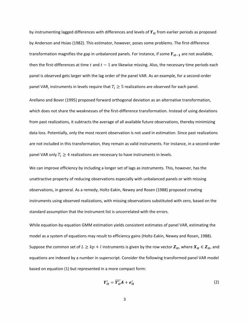
by instrumenting lagged differences with differences and levels of ��� from earlier periods as proposed

by Anderson and Hsiao (1982). This estimator, however, poses some problems. The first-difference

transformation magnifies the gap in unbalanced panels. For instance, if some ����� are not available,

then the first-differences at time � and � − 1 are likewise missing. Also, the necessary time periods each

panel is observed gets larger with the lag order of the panel VAR. As an example, for a second-order

panel VAR, instruments in levels require that �� ≥ 5 realizations are observed for each panel.

Arellano and Bover (1995) proposed forward orthogonal deviation as an alternative transformation,

which does not share the weaknesses of the first-difference transformation. Instead of using deviations

from past realizations, it subtracts the average of all available future observations, thereby minimizing

data loss. Potentially, only the most recent observation is not used in estimation. Since past realizations

are not included in this transformation, they remain as valid instruments. For instance, in a second-order

panel VAR only �� ≥ 4 realizations are necessary to have instruments in levels.

We can improve efficiency by including a longer set of lags as instruments. This, however, has the

unattractive property of reducing observations especially with unbalanced panels or with missing

observations, in general. As a remedy, Holtz-Eakin, Newey and Rosen (1988) proposed creating

instruments using observed realizations, with missing observations substituted with zero, based on the

standard assumption that the instrument list is uncorrelated with the errors.

While equation-by-equation GMM estimation yields consistent estimates of panel VAR, estimating the

model as a system of equations may result to efficiency gains (Holtz-Eakin, Newey and Rosen, 1988).

Suppose the common set of � ≥ �� + � instruments is given by the row vector ���, where ��� ∈ ���, and

equations are indexed by a number in superscript. Consider the following transformed panel VAR model

based on equation (1) but represented in a more compact form:

���∗ = ���

∗����� + ���∗ (2)

4

���∗ = ����

�∗ ����∗ … ���

���∗ ����∗ �

���∗���� = [�����

∗ �����∗ … �������

∗ �����∗ ���

∗ ]

���∗ = ����

�∗ ����∗ … ���

���∗ ����∗ �

�′ = ���′ ��′ … ����� ��′ �′�

where the asterisk denotes some transformation of the original variable. If we denote the original

variable as ���, then the first difference transformation imply that ���∗ = ��� − �����, while for the

forward orthogonal deviation ��� = (��� − ��������)����/(��� + 1) , where ��� is the number of available

future observations for panel � at time �, and �������� is its average.

Suppose we stack observations over panels then over time. The GMM estimator is given by

� = ��∗���′� � � �′�∗������

(�∗���′� � � �′�∗) (3)

where � � is a (� � �) weighting matrix assumed to be non-singular, symmetric and positive semi-

definite. Assuming that �[���]= � and rank ���∗������ = �� + �, the GMM estimator is consistent. The

weighting matrix � � may be selected to maximize efficiency (Hansen, 1982).5

Joint estimation of the system of equations makes cross-equation hypothesis testing straightforward.

Wald tests about the parameters may be implemented based on the GMM estimate of � and its

covariance matrix. Granger causality tests, with the hypothesis that all coefficients on the lag of variable

� are jointly zero in the equation for variable �, may likewise be carried out using this test.

5 Roodman (2009) provides an excellent discussion of GMM estimation in a dynamic panel setting and its

applications using Stata. Readers are encouraged to read his paper for a more detailed discussion of this topic.

5

2.2. Model Selection

Panel VAR analysis is predicated upon choosing the optimal lag order in both panel VAR specification

and moment condition. Andrews and Lu (2001) proposed consistent moment and model selection

criteria (MMSC) for GMM models based on Hansen’s (1982) � statistic of over-identifying restrictions.

Their proposed MMSC are analogous to various commonly used maximum likelihood-based model

selection criteria, namely the Akaike information criteria (AIC) (Akaike, 1969), the Bayesian information

criteria (BIC) (Schwarz, 1978; Rissanen, 1978; Akaike, 1977), and the Hannan-Quinn information criteria

(HQIC) (Hannan and Quinn, 1979).

Applying Andrews and Lu’s MMSC to the GMM estimator in (3), their proposed criteria select the pair of

vectors (�,�) that minimizes

�������,�(�,�,�)= ��(���,���)− (|�| − |�|)�� ln � (4)

�������,�(�,�,�)= ��(���,���)− 2��(|�| − |�|) (5)

��������,�(�,�)= ��(���,���)− ���(|�| − |�|)ln ln � , � > 2 (6)

where ��(�,�,�) is the � statistic of over-identifying restriction for a �-variate panel VAR of order � and

moment conditions based on � lags of the dependent variables with sample size �.

By construction, the above MMSC are available only when � > �. As an alternative criterion, the overall

coefficient of determination (CD) may be calculated even with just-identified GMM models. Suppose we

denote the (� � �) unconstrained covariance matrix of the dependent variables by �. CD captures the

proportion of variation explained by the panel VAR model, and may be calculated as

�� = 1 −det(�)

det(�) (7)

6

2.3. Impulse Response

Without loss of generality, we drop the exogenous variables in our notation and focus on the

autoregressive structure of the panel VAR in equation (1). Lutkepohl (2005) and Hamilton (1994) both

show that a VAR model is stable if all moduli of the companion matrix �� are strictly less than one, where

the companion matrix is formed by

�� =

⎣⎢⎢⎢⎡�� �� ⋯ �� ����

�� �� ⋯ �� ��

�� �� ⋯ �� ��

⋮ ⋮ ⋱ ⋮ ⋮�� �� ⋯ �� �� ⎦

⎥⎥⎥⎤

(8)

Stability implies that the panel VAR is invertible and has an infinite-order vector moving-average (VMA)

representation, providing known interpretation to estimated impulse-response functions and forecast-

error variance decompositions. The simple impulse-response function �� may be computed by rewriting

the model as an infinite vector moving-average, where �� are the VMA parameters.

�� = �

�� , � = �

� ������

�

���

, � = �,�,. . (9)

The simple IRFs have no causal interpretation, however. Since the innovations ��� are correlated

contemporaneously, a shock on one variable is likely to be accompanied by shocks in other variables, as

well. Suppose we have a matrix �, such that �′� = �. Then � may be used to orthogonalize the

innovations as ������ and to transform the VMA parameters into the orthogonalized impulse-responses

���. The matrix � effectively imposes identification restrictions on the system of dynamic equations.

Sims (1980) proposed the Cholesky decomposition of � to impose a recursive structure on a VAR. The

decomposition however is not unique, but depends on the ordering of variables in �.

7

Impulse-response function confidence intervals may be derived analytically based on the asymptotic

distribution of the panel VAR parameters and the cross-equation error variance-covariance matrix.

Alternatively, the confidence interval may likewise be estimated using Monte Carlo simulation, and

bootstrap resampling methods.6

2.4. Forecast-error variance decomposition

The ℎ-step ahead forecast-error can be expressed as

����� − �[�����]= � ��(�����)��

���

���

(10)

where ����� is the observed vector at time � + ℎ and �[�����] is the ℎ-step ahead predicted vector

made at time �. Similar to impulse-response functions, we orthogonalize the shocks using the matrix �

to isolate each variable’s contribution to the forecast-error variance. The orthogonalized shocks ������

have a covariance matrix ��, which allows straightforward decomposition of the forecast-error variance.

More specifically, the contribution of a variable � to the ℎ-step ahead forecast-error variance of

variable � may be calculated as

� ����

���

���

= �(��� �����)�

���

���

(11)

where �� is the �-th column of ��. In application, the contributions are often normalized relative to the

ℎ-step ahead forecast-error variance of variable �

� �.��

���

���

= � ��� ��′�����

���

���

(12)

6 See for instance Lutkepohl (2005) for details applied in time-series VAR.

8

Similar to impulse-response functions, confidence intervals may be derived analytically or estimated

using various resampling techniques.

3. Stata syntax

Model selection, estimation and inference about the panel vector autoregression model above can be

implemented with the new Stata commands pvar, pvarsoc, pvargranger, pvarstable, pvarirf

and pvarfevd. The syntax and outputs are closely patterned after Stata’s built-in var commands for

ease of use in switching between panel and time series VAR. We describe the commands’ syntax in this

section and provide examples in section 4.

3.1. pvar

pvar estimates panel vector autoregression models by fitting a multivariate panel regression of each

dependent variable on lags of itself, lags of all other dependent variables and exogenous variables, if

any. The estimation is by generalized method of moments (GMM). The command is implemented using

the interactive version of Stata’s gmm with analytic derivatives.

Syntax

pvar depvarlist [if] [in] [, options]

Options

lags(#) specifies the maximum lag order # to be included in the model. The default is to use the first

lag of each variable in depvarlist.

exog(varlist) specifies a list of exogenous variables to be included in the panel VAR.

9

fod and fd specifies how the panel-specific fixed effects will be removed. fod specifies that the panel

fixed-effects be removed using forward orthogonal deviation or Helmert transformation. By

default, the first # lags of transformed depvarlist in the model are instrumented by the same

lags in level (i.e. untranformed). fod is the default option. fd specifies that the panel-specific

fixed effects be removed using first difference instead of forward orthogonal deviations. By

default, the first # lags of transformed (i.e. differenced) depvarlist in the model are

instrumented by the #+1 to 2#+1 lags of depvarlist in levels (i.e. untransformed).

td subtracts from each variable in the model its cross-sectional mean before estimation. This could be

used to removed time fixed effects from all the variables prior to any other transformation.

instlags(numlist) overrides the default lag orders of depvarlist used as instruments in the

model (see fod and fd options above which describe which lags are used as default). Instead the

numlist-th lags are used as instruments.

gmmstyle specifies that "GMM-style" instruments as proposed by Holtz-Eakin, Newey and Rosen

(1988) be used. For each instrument based on lags of depvarlist, missing values are substituted

with zero. Observations with no valid instruments are excluded. This option is available only with

instlags().

gmmopts(options) overrides the default gmm options run by pvar. Each equation in the model may

be accessed individually using the variable names in depvarlist as equation names.

vce(vcetype[, independent]) specifies the type of standard error reported, which includes types

that are robust to some types of misspecification, that allow for intragroup correlation, and that

use bootstrap or jackknife methods.

overid specifies that Hansen's J statistic of over-identifying restriction be reported. This option is

available only for over-identified systems.

10

level(#) specifies the confidence level, as a percentage, to be used for reporting confidence intervals.

The default is level(95) or as set by set level.

noprint suppresses printing of the coefficient table.

Saved Results

pvar saves the following in e():

Scalars

e(N) number of observations

e(n) number of panels

e(tmin) first time period in sample

e(tmax) last time period in sample

e(tbar) average time periods among panels

e(mlag) maximum lag order in panel VAR

e(N_clust) number of clusters

e(Q) criterion function

e(J) Hansen's J chi-squared statistic

e(J_df) J statistic degrees of freedom

e(rank) rank of e(V)

e(ic) number of iterations used by iterative GMM estimator

e(converged)1 if converged, 0 otherwise

Macros

e(cmd) pvar

e(cmdline) command as typed

11

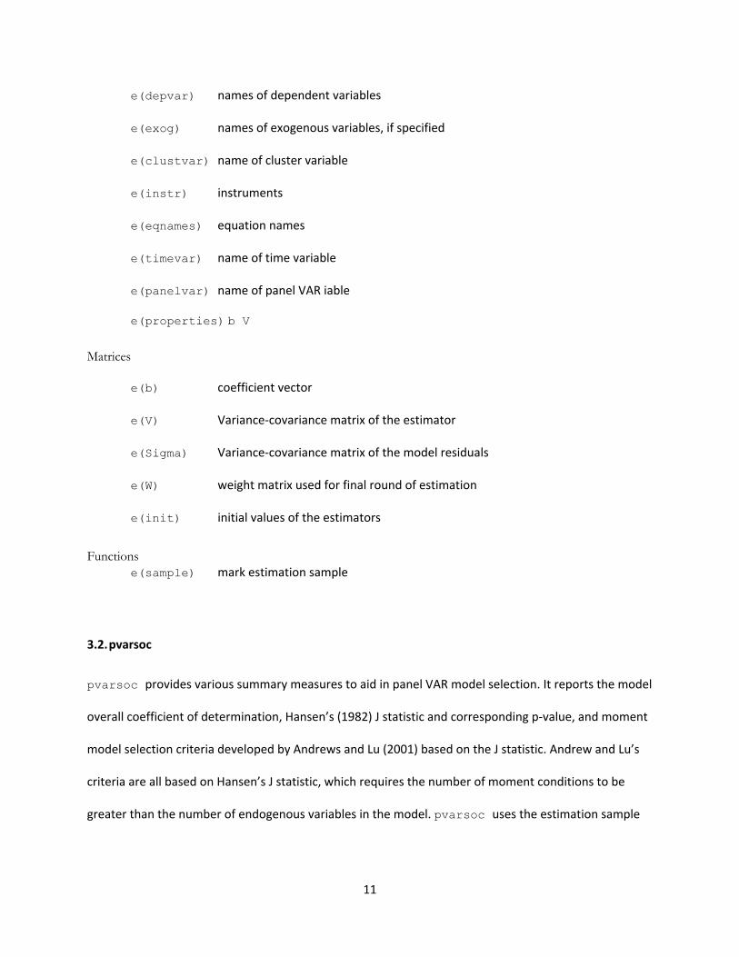
e(depvar) names of dependent variables

e(exog) names of exogenous variables, if specified

e(clustvar) name of cluster variable

e(instr) instruments

e(eqnames) equation names

e(timevar) name of time variable

e(panelvar) name of panel VAR iable

e(properties) b V

Matrices

e(b) coefficient vector

e(V) Variance-covariance matrix of the estimator

e(Sigma) Variance-covariance matrix of the model residuals

e(W) weight matrix used for final round of estimation

e(init) initial values of the estimators

Functions e(sample) mark estimation sample

3.2. pvarsoc

pvarsoc provides various summary measures to aid in panel VAR model selection. It reports the model

overall coefficient of determination, Hansen’s (1982) J statistic and corresponding p-value, and moment

model selection criteria developed by Andrews and Lu (2001) based on the J statistic. Andrew and Lu’s

criteria are all based on Hansen’s J statistic, which requires the number of moment conditions to be

greater than the number of endogenous variables in the model. pvarsoc uses the estimation sample

12

of the least restrictive panel VAR model, i.e. with the highest lag order used, for all models that would

be estimated by the program.

Syntax

pvarsoc depvarlist [if] [in] [, options]

Options

maxlag(#) specifies the maximum lag order for which the statistics are obtained.

pinstlag(numlist) specifies that the numlist-th lag from the highest lag order of depvarlist

specified in the panel VAR model implemented using pvar be used. This option cannot be

specified with the option pvaropts(instlag(numlist)).

pvaropts(options) passes arguments to pvar. All arguments specified in options are passed to

and used by pvar in estimation.

Saved Results

pvarsoc saves the following in r():

Scalars

r(N) number of observations

r(n) number of panels

r(tmin) first time period in sample

r(tmax) last time period in sample

r(tbar) average time periods among panels

r(maxlag) maximum lag order in panel VAR

Macros

r(endog) names of endogenous variables

13

r(exog) names of exogenous variables, if specified

Matrices

r(stats) CD, J and p-value, MBIC, MAIC, and MQIC

3.3. pvargranger

The post-estimation command pvargranger performs Granger causality Wald tests for each equation

of the underlying panel VAR model. It provides a convenient alternative to Stata’s built-in test

command.

Syntax

pvargranger [, estimates(estname)]

Options

estimates(estname) requests that pvargranger use the previously obtained set of panel VAR

estimates saved as estname. By default, pvargranger uses the active (i.e. the latest) results.

Saved Results

pvargranger saves the following in r():

Matrix

r(pgstats) chi-squared, degrees of freedom, and p-values

3.4. pvarstable

The post-estimation command pvarstable checks the stability condition of panel VAR estimates by

calculating the modulus of each eigenvalue of the estimated model. Lutkepohl (2005) and Hamilton

(1994) both show that a VAR model is stable if all moduli of the companion matrix are strictly less than

one. Stability implies that the panel VAR is invertible and has an infinite-order vector moving-average

14

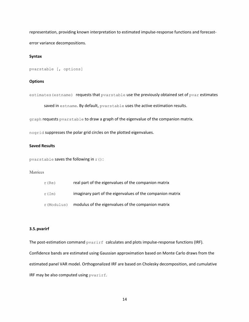
representation, providing known interpretation to estimated impulse-response functions and forecast-

error variance decompositions.

Syntax

pvarstable [, options]

Options

estimates(estname) requests that pvarstable use the previously obtained set of pvar estimates

saved in estname. By default, pvarstable uses the active estimation results.

graph requests pvarstable to draw a graph of the eigenvalue of the companion matrix.

nogrid suppresses the polar grid circles on the plotted eigenvalues.

Saved Results

pvarstable saves the following in r():

Matrices

r(Re) real part of the eigenvalues of the companion matrix

r(Im) imaginary part of the eigenvalues of the companion matrix

r(Modulus) modulus of the eigenvalues of the companion matrix

3.5. pvarirf

The post-estimation command pvarirf calculates and plots impulse-response functions (IRF).

Confidence bands are estimated using Gaussian approximation based on Monte Carlo draws from the

estimated panel VAR model. Orthogonalized IRF are based on Cholesky decomposition, and cumulative

IRF may be also computed using pvarirf.

15

Syntax

pvarirf [, options]

Options

step(#) specifies the step (forecast) horizon; the default is ten periods.

impulse(impulsevars) and response(endogvars) specify the impulse and response variables.

Usually one of each is specified, and one graph is drawn. If multiple variables are specified, a

separate subgraph is drawn for each impulse-response combination. If impulse() and

response() are not specified, subgraphs are drawn for all combinations of impulse and

response variables.

porder(varlist) specifies the Cholesky ordering of the endogenous variables to be used when

estimating orthogonalized IRFs, as well as the order of the IRF plots. By default, the order in

which the variables were originally specified on the pvar command is used. This allows a new

set of IRFs with a different order to be produced without re-estimating the system.

oirf requests that orthogonalized IRFs be estimated. The default is simple IRFs.

cumulative computes cumulative impulse response functions. This option may be combined with

oirf.

mc(#) requests that # Monte Carlo draws be used to estimate the confidence intervals of the IRFs using

Gaussian approximation. The default is not to plot confidence intervals, i.e. # = 0.

table displays the calculated impulse-response functions as a table. The default is not to tabulate IRFs.

level(#)specifies the confidence level, as a percentage, to be used for computing confidence bands.

The default is level(95) or as set by set level. level is available only when mc(#)> 1 is

specified.

16

dots requests the display of iteration dots. By default, one dot character is displayed for each iteration.

A red 'x' is displayed if the iteration returns an error.

save(filename) specifies that the calculated IRFs be saved under the name filename.

byoption(by_option) affects how the subgraphs are combined, labeled, etc. This option is

documented in [G] by_option.

nodraw suppresses the display of the estimated IRFs.

Saved Results

pvarirf saves the following in r():

Scalars

r(iter) Monte Carlo iterations

r(step) forecast horizon

Macros

r(porder) Cholesky order of orthogonalized IRF

3.6. pvarfevd

The post-estimation command pvarfevd computes forecast-error variance decomposition (FEVD)

based on a Cholesky decomposition of the residual covariance matrix of the underlying panel VAR

model. Standard errors and confidence intervals based on Monte Carlo simulation may be optionally

computed.

Caution in interpreting computed FEVD should be exercised when exogenous variables are included in

the underlying panel VAR model. Contributions of exogenous variables, when included in the panel VAR

model, to forecast-error variance are disregarded in calculating FEVD.

17

Syntax

pvarfevd [, options]

Options

step(#) specifies the step (forecast) horizon; the default is ten periods.

impulse(impulsevars) and response(responsevars) specify the impulse and response

variables for which forecast-error variance decomposition are to be reported. If impulse() or

response() is not specified, each endogenous variable, in turn, is used.

porder(varlist) specifies the Cholesky ordering of the endogenous variables to be used when

estimating FEVDs. By default, the order in which the variables were originally specified on the

underlying pvar command is used.

mc(#) requests that # Monte Carlo draws be used to estimate the standard errors and the percentile-

based 90% confidence intervals of the FEVDs. Computed standard errors and confidence

intervals are not displayed, but may be saved as a separate file.

dots requests the display of iteration dots. By default, one dot character is displayed for each iteration.

A red 'x' is displayed if the iteration returns an error.

save(filename) specifies that the FEVDs be saved under the name filename. In addition, standard

errors and percentile-based 90% confidence intervals are saved when #>1 in option mc(#) is

specified.

notable requests the table to be constructed but not displayed.

Saved Results

pvarfevd saves the following in r():

18

Scalars

r(iter) Monte Carlo iterations

r(step) forecast horizon

Macros

r(porder) Cholesky order

4. Examples

We illustrate the use of the pvar suite of commands by analyzing the relationship between annual

hours worked and hourly earnings, which has been previously analyzed by Holtz-Eakin, Newey and

Rosen (1988) on their seminal paper on panel vector autoregression. To compare our new programs

with Stata’s built-in var suite of commands, we also applied the new pvar suite of commands to

Lutkephol’s (1993) West Germany time series data.

4.1. National Longitudinal Survey data

We use the subsample of women aged 14-26 years in 1968 from the National Longitudinal Surveys of

1968 to 1978 available from Stata. Our subsample consists of 2,039 women who had reported wages

(wage) and annual hours worked (hours) in at least three rounds of the survey, of which two are in

consecutive years. Holtz-Eakin, et. al. used the same survey but with a different time period and

different subsample of workers, thus results may not be directly comparable.

Model selection measures calculated using pvarsoc for first- to third-order panel VAR s using the first

four lags of hours and wage as instruments is shown below.

19

Based on the three model selection criteria by Andrews and Lu (2001) and the over-all coefficient of

determination, first-order panel VAR is the preferred model, since this has the smallest MBIC, MAIC and

MQIC. While we also want to minimize Hansen’s J statistic, it does not correct for the degrees of

freedom in the model like the model and moment selection criteria by Andrews and Lu. Based on the

selection criteria, we fit a first-order panel VAR model with the same specification of instruments as

above using GMM estimation implemented by pvar.

3 .9862297 3.624628 .4591831 -23.29944 -4.375372 -11.62918 2 .988392 5.395145 .7146273 -48.453 -10.60486 -25.11248 1 .9906918 11.74496 .4663737 -69.02726 -12.25504 -34.01648 lag CD J J pvalue MBIC MAIC MQIC

Ave. no. of T = 1.656 No. of panels = 506 Sample: 72 - 73 No. of obs = 838 Selection order criteria

...Running panel VAR lag order selection on estimation sample. pvarsoc wage hours, maxlag(3) pvaropts(instl(1/4))

. gen wage = exp(ln_wage)

(National Longitudinal Survey. Young Women 14-26 years of age in 1968). webuse nlswork2

Instruments : l(1/4).(wage hours) L1. .5834965 .1436703 4.06 0.000 .3019079 .865085 hours L1. -.0575627 .5706831 -0.10 0.920 -1.176081 1.060956 wage hours L1. .0170489 .0176144 0.97 0.333 -.0174747 .0515725 hours L1. .6428702 .0978213 6.57 0.000 .4511439 .8345965 wage wage Coef. Std. Err. z P>|z| [95% Conf. Interval]

Ave. no. of T = 1.656 No. of panels = 506 No. of obs = 838GMM weight matrix: RobustInitial weight matrix: IdentityFinal GMM Criterion Q(b) = .014

GMM Estimation

Panel vector autoregresssion

. pvar wage hours, instl(1/4)

20

Note that the 506 women included in the estimation is significantly less than the full subsample of

women available in the data. By default, pvar drops from estimation any observation with missing data.

Since hours worked and wages are not observed in all years for all women in the subsample the number

of observations dropped grows with the lag order of variables included as instruments. We can improve

estimation by using “GMM-style” instruments as proposed by Holtz-Eakin, et. al. Instrument lags with

missing values are replaced with zeroes. This increases the estimation sample, which results to more

efficient estimates.

Although Granger causality for a first-order panel VAR may be inferred from the pvar output above, we

still perform the test using pvargranger as an illustration. Results of the Granger causality tests below

show that wage Granger-causes hours, and hours Granger-causes wage at the usual confidence levels,

similar to the findings by Holtz-Eakin, et.al.

Instruments : l(1/4).(wage hours) L1. -.1068443 .0947648 -1.13 0.260 -.2925799 .0788912 hours L1. -2.280437 .3250711 -7.02 0.000 -2.917565 -1.643309 wage hours L1. .0721378 .0248413 2.90 0.004 .0234498 .1208257 hours L1. .8062972 .079843 10.10 0.000 .6498078 .9627867 wage wage Coef. Std. Err. z P>|z| [95% Conf. Interval]

Ave. no. of T = 2.578 No. of panels = 2039 No. of obs = 5257GMM weight matrix: RobustInitial weight matrix: IdentityFinal GMM Criterion Q(b) = .00792

GMM Estimation

Panel vector autoregresssion

. pvar wage hours, instl(1/4) gmmstyle

21

Panel vector autoregression model estimates are seldom interpreted by its self. In practice, researchers

are often interested in the impact of exogenous changes in each endogenous variable to other variables

in the panel VAR system. Prior to estimating impulse-response functions (IRF) and forecast-error

variance decompositions (FEVD), however, we first check the stability condition of the estimated panel

VAR. The resulting table and graph of eigenvalues confirms that the estimate is stable.

ALL 49.213 1 0.000 wage 49.213 1 0.000 hours ALL 8.433 1 0.004 hours 8.433 1 0.004 wage Equation \ Excluded chi2 df Prob > chi2

Ha: Excluded variable Granger-causes Equation variable Ho: Excluded variable does not Granger-cause Equation variable panel VAR-Granger causality Wald test

. pvargranger

pVAR satisfies stability condition. All the eigenvalues lie inside the unit circle.

.1400809 0 .1400809 .559372 0 .559372 Real Imaginary Modulus Eigenvalue

Eigenvalue stability condition

. pvarstable, graph

-1-.

50

.51

Imag

inary

-1 -.5 0 .5 1Real

Roots of the companion matrix

22

Following the theoretical exposition by Holtz-Eakin, et. al., we argue that shocks in wage levels have

direct impact on contemporaneous hours worked, while current work effort affects wages only in the

future. Using this causal ordering, we calculated the implied IRF using pvarirf and the implied FEVD

using pvarfevd. The IRF confidence intervals are computed using 200 Monte Carlo draws based on the

estimated model. Standard errors and confidence intervals for the FEVD estimates are likewise available

but not shown here to save on space.

. pvarirf, mc(200) oirf byopt(yrescale)

fevd.dtaon 200 Monte Carlo simulations are saved in fileFEVD standard errors and confidence intervals based 10 .4039508 .5960492 9 .4039355 .5960644 8 .4038868 .5961132 7 .403731 .596269 6 .4032323 .5967677 5 .4016319 .598368 4 .3964525 .6035476 3 .3792638 .6207362 2 .3183373 .6816627 1 .0933682 .9066318 0 0 0hours 10 .9402192 .0597809 9 .9402227 .0597773 8 .9402341 .059766 7 .9402702 .0597298 6 .9403861 .0596139 5 .9407574 .0592426 4 .9419529 .0580471 3 .945842 .054158 2 .9587072 .0412928 1 1 0 0 0 0wage horizon wage hoursForecast Impulse variable and variable Response

Forecast-error variance decomposition

note: label truncated to 80 characters. pvarfevd, mc(200) save("fevd.dta")

23

Based on the FEVD estimates, we see that as much as 40 percent of variation in hours worked by

women in our example can be explained by their wages. On the other hand, hours workedexplain only

five percent of variation in future wages of women. In terms of levels, the IRF plot shows that a positive

shock on real wages leads to a decreased work effort, which implies a backward bending labor supply

among women in the sample. It is also noteworthy that current shock in work effort have positive yet

short-lived impacts on both hours worked and wages. The effect of current shock on wages, on the

other hand, has a persistent positive impact on future wages.

4.2. Lutkepohl (1993) West Germany data

We compare our pvar command with the built-in Stata var command using Lutkepohl’s West Germany

time series data available from Stata. The data contains first difference of the natural log of investment

(dln_inv), of income (dln_inc), and of consumption (dln_consump) from the second quarter of 1962 up

to the fourth quarter of 1982. Lutkepohl uses only observations up to the fourth quarter of 1978 in his

-2

0

2

4

-4

-3

-2

-1

0

0

.2

.4

.6

0

.5

1

1.5

0 5 10 0 5 10

hours : hours

wage : hours

hours : wage

wage : wage

95% CI Orthogonalized IRF

step

impulse : response

24

examples, but we use the full sample in our exposition here. We set the time-series data as a one-panel

data for pvar to function.

For simplicity, we compare VAR(1) estimates using the built-in Stata var (denoted var1 in the output

below), and two specifications of the new Stata command pvar: 1) using the default options with a one-

lag instruments (pvar1_1) and 2) using a five-lags “GMM style” instrument set (pvar1_5). The

VAR/panel VAR point estimates are summarized as a table below. Based on the point estimates and

standard errors calculated, notice that each coefficient’s 95 percent confidence interval, i.e. roughly two

standard errors on either side of the point estimate, overlap across estimators. Also, pvar uses one less

observation than var because of the forward orthogonal transformation.

delta: 1 quarter time variable: qtr, 1960q1 to 1982q4 panel variable: id (strongly balanced). xtset id qtr

. gen id = 1

(Quarterly SA West German macro data, Bil DM, from Lutkepohl 1993 Table E.1). webuse lutkepohl2

25

Cholesky impulse-response functions and forecast-error variance decompositions can likewise be

estimated using the new Stata commands pvarirf and pvarfevd, but are not shown in the interest of

space.7 Similar to the VAR/panel VAR point estimates, the 95 percent confidence intervals of the

7 This paper is accompanied with a *.do file which details all commands used in this paper.

legend: b/se tmax 91 90 90 tmin 2 2 2 N 90 89 89 Statistics .12186649 .1430883 .13304683 L1. -.20676573 -.03995971 -.21808259 dln_consump .10729047 .14926382 .13852001 L1. .30784668 .41644295 .7993262 dln_inc .02590542 .02349897 .01656548 L1. -.00139181 -.00633585 -.00875257 dln_inv dln_consump .13274394 .14565136 .12359724 L1. .23605129 .41862255 .15905599 dln_consump .11686691 .16229116 .12738437 L1. -.00827691 .12441837 .47762624 dln_inc .02821766 .02586756 .01613904 L1. .0340018 .02621551 .0209324 dln_inv dln_inc .5011716 .52570264 .36813698 L1. .57644709 .72224157 1.6836959 dln_consump .44122824 .45532768 .24411809 L1. .41510931 .56587455 .08242313 dln_inc .10653512 .17654561 .11342286 L1. -.22185123 -.21273369 -.26849009 dln_inv dln_inv Variable var1 pvar1_1 pvar1_5

. est table var1 pvar1_1 pvar1_5, se stat(N tmin tmax) drop(_cons)

. est store pvar1_5

. qui pvar dln_inv dln_inc dln_consump, lags(1) instl(1/5) gmms

. est store pvar1_1

. qui pvar dln_inv dln_inc dln_consump, lags(1)

. est store var1

. qui var dln_inv dln_inc dln_consump, lags(1)

26

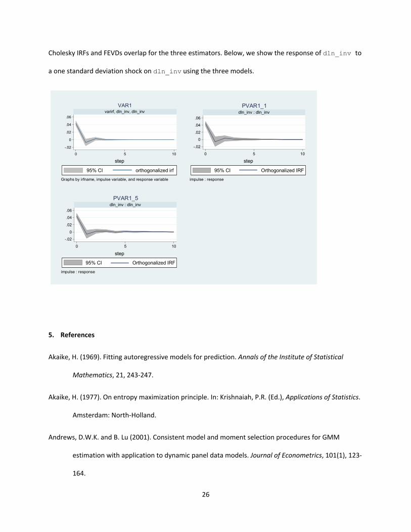
Cholesky IRFs and FEVDs overlap for the three estimators. Below, we show the response of dln_inv to

a one standard deviation shock on dln_inv using the three models.

5. References

Akaike, H. (1969). Fitting autoregressive models for prediction. Annals of the Institute of Statistical

Mathematics, 21, 243-247.

Akaike, H. (1977). On entropy maximization principle. In: Krishnaiah, P.R. (Ed.), Applications of Statistics.

Amsterdam: North-Holland.

Andrews, D.W.K. and B. Lu (2001). Consistent model and moment selection procedures for GMM

estimation with application to dynamic panel data models. Journal of Econometrics, 101(1), 123-

164.

-.02

0

.02

.04

.06

0 5 10

varirf, dln_inv, dln_inv

VAR1

95% CI orthogonalized irf

step

Graphs by irfname, impulse variable, and response variable

-.02

0

.02

.04

.06

0 5 10

dln_inv : dln_inv

PVAR1_1

95% CI Orthogonalized IRF

step

impulse : response

-.02

0

.02

.04

.06

0 5 10

dln_inv : dln_inv

PVAR1_5

95% CI Orthogonalized IRF

step

impulse : response

27

Arellano, M. and O. Bover (1995). Another look at the instrumental variable estimation of error-

components model. Journal of Econometrics, 68(1), 29-51.

Bun, M.J.G. and M.A. Carree (2005). Bias-corrected estimation in dynamic panel data models. Journal of

Business & Economic Statistics, 23(2), 200-210.

Canova, F. and M. Ciccarelli (2013). Panel vector autoregressive models: A survey. Advance in

Econometrics, 32,

Carpenter, S. and S. Demiralp (2012). Money, reserves, and the transmission of monetary policy: Does

the money multiplier exist? Journal of Macroeconomics, 34(1), 59-75.

Everaert, G. and L. Pozzi (2007). Bootstrap-based correction for dynamic panels. Journal of Economic

Dynamics and Control, 31(4), 1160-1184.

Granger, C.W.J. (1969). Investigating causal relations by econometric models and cross-spectral

methods. Econometrica, 37(3), 424-438.

Hamilton, J.D. (1994). Time Series Analysis. Princeton: Princeton University Press.

Hannan, E.J. and B.G. Quinn (1979). The determination of the order of an autoregression. Journal of the

Royal Statistical Society, Series B, 41(2), 190-195.

Hansen, L.P. (1982). Large sample properties of generalized method of moments estimators.

Econometrica, 50(4), 1029-1054.

Head, H. H. Lloyd-Ellis and H. Sun (2015). Search, liquidity, and the dynamics of house prices and

construction. The American Economic Review, 104(4), 1172-1210.

Holtz-Eakin, D., W. Newey and H.S. Rosen (1988). Estimating vector autoregressions with panel data.

Econometrica, 56(6), 1371-1395.

28

Judson, R.A., and A.L. Owen. 1999. Estimating dynamic panel data models: A guide for

macroeconomists. Economics Letters, 65(1), 9-15.

Kiviet, J.F. (1995). On bias, inconsistency, and efficiency of various estimators in dynamic panel data

models. Journal of Econometrics, 68(1), 53-78.

Love, I. and L. Zicchino (2006). Financial development and dynamic investment behavior: Evidence from

panel VAR. The Quarterly Review of Economics and Finance, 46(2), 190-210.

Lutkepohl, H. (1993). Introduction to Multiple Time Series Analysis, 2nd Ed. New York: Springer.

Lutkepohl, H. (2005). New Introduction to Multiple Time Series Analysis. New York: Springer.

Mora, N. and A. Logan (2012). Shocks to bank capital: Evidence from UK banks at home and away.

Applied Economics, 44(9), 1103-1119.

Neumann, T.C., P.V. Fishback and S. Kantor (2010). The dynamics of relief spending and the private

urban market during the New Deal. The Journal of Economic History, 70(1) 195-220.

Nickell, S.J. (1981). Biases in dynamic models with fixed effects. Econometrica, 49(6), 1417-1426.

Risannen, J. (1978). Modeling by shortest data description. Automatica, 14(5), 465-471.

Roodman, D. (2009). How to do xtabond2: An introduction to difference and system GMM in Stata. The

Stata Journal, 9(1), 86-139.

Schwarz, G. (1978). Estimating the dimension of a model. Annals of Statistics, 6(2), 461-464.

Sims, C.A. (1980). Macroeconomics and reality. Econometrica, 48(1), 1-48.