1

Energy-efficient Multicasting of Scalable Video

Streams over WiMAX Networks

Somsubhra Sharangi, Ramesh Krishnamurti, and Mohamed Hefeeda

Abstract

The Multicast/Broadcast Service (MBS) feature of mobile WiMAX network is a promising technol-

ogy for providing wireless multimedia, because it allows the delivery of multimedia content to large-scale

user communities in a cost-efficient manner. In this paper, we consider WiMAX networks that transmit

multiple video streams encoded in scalable manner to mobile receivers using the MBS feature. We

focus on two research problems in such networks: (i) maximizing the video quality and (ii) minimizing

energy consumption for mobile receivers. We formulate and solve the substream selection problem to

maximize the video quality, which arises when multiple scalable video streams are broadcast to mobile

receivers with limited resources. We show that this problem is NP-Complete, and design a polynomial

time approximation algorithm to solve it. We prove that the solutions computed by our algorithm are

always within a small constant factor from the optimal solutions. In addition, we extend our algorithm to

reduce the energy consumption of mobile receivers. This is done by transmitting the selected substreams

in bursts, which allows mobile receivers to turn off their wireless interfaces to save energy. We show how

our algorithm constructs burst transmission schedules that reduce energy consumption without sacrificing

the video quality. Using extensive simulation and mathematical analysis we show that the proposed

algorithm: (i) is efficient in terms of execution time, (ii) achieves high radio resource utilization, (iii)

maximizes the received video quality, and (iv) minimizes the energy consumption for mobile receivers.

Index Terms

Mobile multimedia; wireless scheduling; scalable video coding; WiMAX; energy optimization

This work is partially supported by the Natural Sciences and Engineering Research Council (NSERC) of Canada.

The authors are with the School of Computing Science, Simon Fraser University, Canada (e-mails: ssa121@cs.sfu.ca;

mhefeeda@cs.sfu.ca,ramesh@cs.sfu.ca).

2

I. INTRODUCTION

The demand for mobile multimedia streams has been increasing in the past few years as indicated

by multiple market analysis studies [1], [2]. Multimedia streams can be delivered to mobile devices

over different wireless networks, including 3G, WiFi and WiMAX networks. In this paper, we focus

on multimedia streaming over WiMAX networks, which are specified by the IEEE 802.16 standard [3].

Although some of the currently deployed WiMAX networks are mostly used to provide wireless Internet

access to subscribers, the WiMAX standard supports various network services. One of these services is

the Multicast and Broadcast Service (MBS), which can be used to deliver multimedia traffic to large-

scale user communities. For example, Yota Telecom [4] has recently started a mobile TV service with 25

channels over its 10Mbps mobile WiMAX network, and UDCast [5] has announced plans for developing

broadcast TV service supporting around 50 channels over mobile WiMAX. It is expected that more

WiMAX deployments will offer mobile multimedia services in the near future. Although considerable

amount of work has been done to make these deployments a reality, several research problems remain

to be addressed in order to optimize the quality of the offered multimedia services.

In this paper, we address two important problems in multimedia streaming over WiMAX networks: (i)

maximizing the video quality and (ii) minimizing energy consumption for mobile receivers. In particular,

we consider broadcasting multiple scalable video streams to mobile receivers. A scalable video stream

is composed of multiple layers, where each layer improves the spatial, temporal, or the visual quality of

the rendered video to the user. Because of their flexibility, scalable video streams can efficiently support

heterogeneous receivers, adapt to network conditions, and utilize the available wireless bandwidth. We

mathematically formulate the problem of selecting the best set of substreams (or layers) from the scalable

video streams in order to maximize the quality for mobile receivers. We show that this problem is NP-

Complete. Thus, optimally solving it in real time may not be computationally feasible. We propose an

approximation algorithm that produces near-optimal solutions and runs in real time. We analytically show

that the approximation factor is close to one.

In addition, since many subscribers of the WiMAX multimedia services are expected to be mobile

users with energy-constrained devices such as smart phones, minimizing the energy consumption of these

devices becomes an important problem in order to extend the viewing time. To address this problem,

we extend our algorithm to reduce the energy consumption of mobile receivers. The extended algorithm

first selects the best substreams and then transmits these substreams in bursts. The burst transmission of

the video data enables mobile receivers to turn off their wireless interfaces for longer periods of time in

3

order to save energy. Our algorithm carefully constructs the burst transmission schedules that reduce the

energy consumption without sacrificing the video quality or introducing any buffer overflow or underflow

instances. We rigorously evaluate the proposed algorithm using simulation and mathematical analysis.

Our results show that the proposed algorithm can efficiently run in real time, achieves high utilization

of the wireless bandwidth, minimizes the energy consumption for mobile receivers, and maximizes the

video quality.

The rest of this paper is organized as follows. In Section II, we present a brief background on video

streaming over WiMAX networks, and we summarize the related works in the literature. We state the

substream selection problem and present the analytical formulation for it in Section III. In Section IV,

we present the proposed approximation algorithm to efficiently solve the substream selection problem. In

section V, we present our extended algorithm which reduces the energy consumption for mobile receivers.

Section VI describes our simulation setup and results. Finally, we conclude the paper in Section VII. A

preliminary version of this paper appeared in [6].

II. BACKGROUND AND RELATED WORK

A. Brief Background

A video streaming service over WiMAX networks is composed of three main entities: (i) content source,

(ii) WiMAX base station, and (iii) WiMAX subscribers. Content sources are national TV broadcasters,

local broadcasters, Internet TV operations and other video broadcast service providers. Multimedia

contents are aggregated from different sources and sent to the WiMAX base station. The WiMAX base

station constructs a schedule to transmit the incoming data to the subscribers.

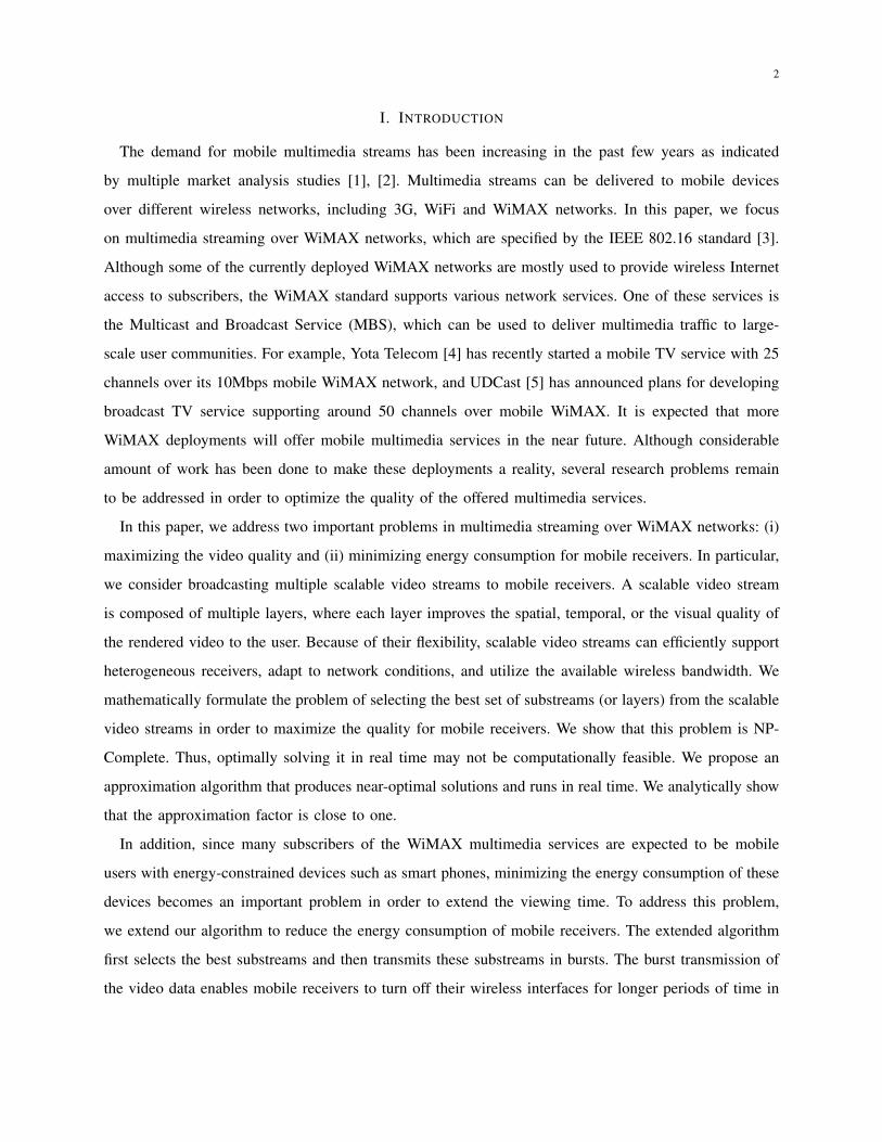
In the WiMAX physical layer, data is transmitted over multiple carriers in Time Division Duplex (TDD)

frames. As illustrated in Figure 1, each frame contains header information and upload/download maps

followed by bursts of user data. Since video dissemination is expected to be a prevalent traffic pattern in

future networks, the WiMAX standard defines a service called Multicast and Broadcast Service (MBS)

in the MAC layer to facilitate broadcast and multicast. Using MBS, a certain area in each TDD frame

can be set aside for multicast-only or broadcast-only data, as shown in Figure 1. The entire frame can

also be designated as a download-only broadcast frame. A major task of the MBS module is to allocate

video data from multiple streams to the MBS data area in each frame such that the real time nature of

all video streams is maintained. Further, the allocation algorithm must consider that the receiver devices

have limited buffer capacity which may cause data loss due to buffer overflow. These constraints impose

stringent QoS and efficiency demands on the allocation algorithm. In the first part of this paper, we

4

Fig. 1. The Frame structure in WiMAX.

present an algorithm to select the best subset of scalable video streams and allocate them in the MBS

area.

The WiMAX standard has defined different sleep mode operations to facilitate power conservation

for mobile subscribers. In the sleep mode operation, the base station informs the mobile subscriber

about the sleep interval, during which the mobile subscriber switches off its RF circuitry. To utilize the

energy conservation mechanism of the sleep mode, the data is sent out in bursts, instead of continuous

transmission. After receiving a burst of data for a short time, receivers go into sleep mode for a pre-

computed period of time. Once we compute a transmission schedule, the sleep intervals for different

streams are embedded in the last frame of a burst. At the start of transmission, each mobile subscriber

receives the first burst and comes to know about its sleep and active intervals. It then accordingly switches

its receiver on or off to receive only the relevant frames. This procedure is continuously repeated for

each scheduling window. In the second part of this paper, we design a burst transmission algorithm to

reduce the energy consumption of mobile devices.

B. Related Work

1) Video Streaming over WiMAX: Wang et al. [7] discuss an architecture for video broadcasting in a

multi-base-station WiMAX system. Their work focuses on coverage and spectral efficiency issues and

considers only temporal video scalability. Cohen et al. [8] combine a group of TDD frames together

into a super-frame. They describe a cost based scheme where a cost function is associated with each

user-channel pair. Three user interaction models are considered: (i) user can either be statically hooked

to a channel, (ii) user can choose to listen to a channel, or (iii) the user channel association can keep

changing based on the transmission medium conditions. The work in [8] does not consider the delay

5

requirements which are central to video streaming. Hosein [9] describes the frame allocation problem for

broadcasting variable bit rate video over WiMAX, but does not consider scalable video content.

Jiang et al. [10] propose a scheme to transmit scalable video streams in which two layers of each video

are transmitted separately. The base layer is transmitted as one stream over a reliable channel while the

enhancement layer is transmitted as a different stream over a less reliable channel. Conceptually, this

work implements a rate adaptive multiple description coding. However, it describes only one stream and

it does not address the resource management problem arising in multi stream transmission scenarios.

Reguant et al. [11] consider splitting a video stream into two streams and transmitting them over two

different broadcast networks. The first stream is transmitted over a DVB-H network at all times while

the second stream is transmitted over WiMAX network most of the time. If the user wants to use some

other non-video application in parallel, the stream going through WiMAX is degraded to accommodate

that application. This ensures a minimum video quality at all times while maintaining the flexibility of

using other applications. While this approach has its benefits, it is not very attractive from a deployment

point of view since the service provider has to install and manage the infrastructure for two different

kinds of networks. Also the solutions described in both [10] and [11] evaluate the performance of video

streaming as an application along with other WiMAX applications and do not utilize MBS. In contrast,

our approach considers a multimedia-intensive system with extensive use of MBS.

2) Energy Efficient Scheduling: Power-aware scheduling schemes for general WiMAX networks have

been proposed in [12], [13], [14], [15]. For example, Seo et al. [12] propose a scheme that utilizes

subscriber information available at the base station. They describe a sleep interval algorithm based on

queuing analysis of the packet arrival rate of subscribers. In contrast, Kim et al. [13] describe a sleep

interval scheme based on the remaining battery life of a mobile subscriber device. Shi et al. [14] propose a

burst scheduling algorithm for energy minimization on per subscriber basis for unicast data. The algorithm

arranges the mobile subscribers in ascending order based on the ratio of the current data arrival rate to the

required data rate. If the current rate is significantly higher than the required rate, the mobile subscriber

can go to sleep for some interval. After computing the sleep intervals for all mobile subscribers the bursts

are scheduled in a longest interval first manner. After transmission of each burst, the algorithm checks

to ensure that the data requirement of all mobile subscribers are being satisfied. The work in [14] is

designed for unicast streaming of video and does not consider the multicast/broadcast service. Also the

algorithm requires maintaining state information of all mobile subscribers served by a base station.

Liao and Lee [15] suggest a scheduling scheme where the uni-cast data is clustered around the multicast

data bursts for increased energy efficiency. They assume that the burst length and positions for a particular

6

stream is the same in all super-frames. Then they present an enhancement to the longest virtual buffer

first scheduling algorithm proposed by Shi et. al. [14] by clustering the unicast data around the multicast

data bursts. Their work evaluates the energy efficiency in a multi-class traffic scenario, whereas our work

is focused on the energy efficiency of the video broadcast service.

III. PROBLEM STATEMENT AND HARDNESS

Our work focuses on optimally utilizing the WiMAX Multicast/Broadcast Service to stream multiple

scalable videos to mobile receivers. In this section, we state the considered problem and show that it is

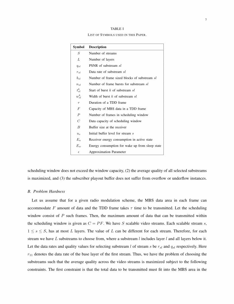
NP-Complete. We also present the mathematical formulation of the problem. For quick reference, we list

all symbols used in the formulation in Table I.

A. Problem Statement

We consider a scenario where a number of scalable video streams are available at a WiMAX base

station. Each stream is to be broadcast using MBS to a group of mobile subscribers. At the WiMAX

base station, the MBS module allocates a fixed-size data area in the download section of each TDD

frame. All video streams are to be allocated only within this MBS data area. As per the mobile WiMAX

standard, each MBS data area can transmit a different amount of data depending on the modulation scheme

chosen, which is in turn selected based on the wireless channel conditions. For broadcast applications,

a common modulation scheme is selected for a group of subscribers. Thus, each MBS area transmits a

fixed amount of data, in effect, creating a fixed bandwidth broadcast channel. We consider a scheduling

window composed of a number of MBS data areas. Data from the video streams are to be allocated to

the MBS areas in the scheduling window. Due to the variable bit rate (VBR) nature of the video streams,

the aggregate data rates may exceed the broadcast channel capacity. Hence, in each scheduling window,

we need to decide which layers to send for each stream. We assume that the base station has enough

buffer space to hold the VBR traffic for one scheduling window. This way, the data rates can be assumed

to be constant during a scheduling window, but they vary across scheduling windows. Since the bit rates

and the receiver buffer states change in each scheduling window, the allocation has to be computed for

every scheduling window. We also assume that all subscribers served by the base station have a fixed

amount of buffer which is used to temporarily store the incoming video data before playing it out. Thus

the optimal substream selection problem we need to solve can be stated as follows.

Problem 1 (Optimal Substream Selection Problem:): Select the optimal subset of layers from each

scalable stream to broadcast over a WiMAX network such that: (1) the total data transmitted in a

7

TABLE I

LIST OF SYMBOLS USED IN THIS PAPER.

Symbol Description

S Number of streams

L Number of layers

qsl PSNR of substream sl

rsl Data rate of substream sl

bsl Number of frame sized blocks of substream sl

nsl Number of frame bursts for substream sl

tk

sl Start of burst k of substream sl

wk

sl Width of burst k of substream sl

τ Duration of a TDD frame

F Capacity of MBS data in a TDD frame

P Number of frames in scheduling window

C Data capacity of scheduling window

B Buffer size at the receiver

us Initial buffer level for stream s

Ea Receiver energy consumption in active state

Ew Energy consumption for wake up from sleep state

ǫ Approximation Parameter

scheduling window does not exceed the window capacity, (2) the average quality of all selected substreams

is maximized, and (3) the subscriber playout buffer does not suffer from overflow or underflow instances.

B. Problem Hardness

Let us assume that for a given radio modulation scheme, the MBS data area in each frame can

accommodate F amount of data and the TDD frame takes τ time to be transmitted. Let the scheduling

window consist of P such frames. Then, the maximum amount of data that can be transmitted within

the scheduling window is given as C = PF . We have S scalable video streams. Each scalable stream s,

1 ≤ s ≤ S, has at most L layers. The value of L can be different for each stream. Therefore, for each

stream we have L substreams to choose from, where a substream l includes layer l and all layers below it.

Let the data rates and quality values for selecting substream l of stream s be rsl and qsl respectively. Here

r11 denotes the data rate of the base layer of the first stream. Thus, we have the problem of choosing the

substreams such that the average quality across the video streams is maximized subject to the following

constraints. The first constraint is that the total data to be transmitted must fit into the MBS area in the

8

current scheduling window. The second constraint is that the buffers at the subscribers must not run out

of data anytime during the scheduling window, and the third constraint is that the base layer of each

stream must be transmitted to guarantee a basic service level agreement.

Theorem 1: The Optimal Substream Selection Problem is NP-Complete.

Proof: First, we consider a relaxed version of the problem with no buffer overflow or underflow

constraints. Thus, we are left with the problem of selecting the substreams such that the average quality

is maximized. We assume that in each scheduling window at least all the base layer streams have to be

transmitted due to service level agreement. Thus, we further modify the problem by eliminating the base

layer constraints, which can be trivially done by reducing the scheduling window capacity by the sum of

data rates of all base layers. Therefore, the modified data capacity can be given as C ′ = C −∑

s∈S rs1.

Now we are left with the problem of deciding which substreams to chose from each stream. We

show that this problem is equivalent to the NP-Complete 0-1 Multiple Choice Knapsack Problem (0-1-

MCKP) [16], which is defined as follows. There are M classes N1, . . . , NM of items to pack in some

knapsack of capacity W . Each item (i, j), where i ∈ M, j ∈ Ni, has a profit p(i, j) and a weight w(i, j).

The problem is to choose at most one item from each class such that the profit sum is maximized without

having the total weight exceed W . We reduce the 0-1-MCKP problem to the Optimal Substream Selection

problem in polynomial time as follows. We make the data rates of choosing a substream represent the item

weight and the corresponding quality values represent the profit of choosing an item. We also make the

streams represent the multiple choice classes and the scheduling window capacity represent the knapsack

capacity. Thus, we have an MCKP instance with S classes, L−1 items per class and a knapsack capacity

of C ′. This means that an efficient solution for the simplified Optimal Substream Selection Problem could

be employed to efficiently solve the NP-Complete 0-1-MCKP problem. In other words, the substream

selection problem is NP-Hard.

In addition, clearly a solution for the simplified Optimal Substream Selection Problem can be verified

in polynomial time. Thus the simplified Optimal Substream Selection Problem is NP-Complete. Conse-

quently, the more general Optimal Substream Selection Problem subject to buffer overflow and underflow

constraints is also NP-Complete.

C. Mathematical Formulation

We assume that all subscribers have B amount of buffer available for the video streaming application

and the data rate and quality values for all substreams of each stream are known ahead of the scheduling

window. This information can either be obtained as a separate meta data for each stream or if the scalable

9

video is encoded using H.264/SVC [17] and the base station is media-aware, this information can be

obtained directly from the encoded video stream itself using the Supplementary Enhancement Information

(SEI) messages. Let the data rate values of substreams be {rs1, rs2, . . . , rSL} and the corresponding

quality values be {qs1, qs2, . . . , qSL}. Each scheduling window is of duration τP . If substream l of

stream s is selected, the amount of data to be transmitted during a scheduling window can be given as

τPrsl. Let binary variables xsl take the value 1 if substream l of stream s is selected for transmission

in the current scheduling window and 0 otherwise. For a substream, we define a burst as a consecutive

set of MBS data areas allocated to the substream in the scheduling window. For any schedule, let nsl be

the number of bursts for substream l of stream s. We denote by variables tksl the starting frame number

and by variable wksl the number of MBS data areas in burst k for substream l of stream s.

The solution of the optimum substream selection problem should generate a list < l, n, < t1sl, w1sl >

, . . . , < tnsl, wnsl >> for each stream. In the list, l denotes the selected substream, n denotes the number of

bursts required for transmitting substream l, and < tksl, wksl > denote the starting point and width of burst

k, respectively. For a subscriber receiving channel s, let the buffer level at the beginning of scheduling

window be us. We need to ensure that all data received during a scheduling window are also consumed

in the same window. In other words F∑nsl

k=1 wksl = τPrsl. At the same time we need to ensure that

buffer overflow and underflow do not occur. At the end of each burst, the total data received is given

by F∑k

i=1 wisl. During that period the total data consumed is given by τ(tksl + wk

sl)rsl. Now in order

to avoid underflow, the difference of these two terms must be greater than zero for all bursts. Similarly,

the overflow conditions can be applied by constraining the difference to be never greater than B. Our

objective is to maximize the average video quality over all the streams. We use the Peak Signal to Noise

Ratio (PSNR) values of the streams to denote quality and take an arithmetic average of the PSNRs of

the selected streams to denote the average video quality. Let us assume that the data to be transmitted

for each substream can be divided into bsl number of F sized data blocks. In other words, rsl = bslF .

Consequently, we have the following optimization problem.

Maximize1

S

S∑

s=1

L∑

l=1

xslqsl (P1)

such that

S∑

s=1

L∑

l=1

xslbsl ≤ P (1a)

L∑

l=1

xsl ≤ 1 (1b)

10

us +k

∑

i=1

wislF − τ(tksl + wk

sl)rsl ≤ B (1c)

us +k−1∑

i=1

wislF − τ(tk−1

sl + wk−1sl )rsl ≥ 0 (1d)

[tksl . . . tksl + wk

sl] ∩ [tksl

. . . tksl

+ wksl] = ∅ (1e)

nsl∑

k=1

wks = xslbsl (1f)

In the above formulation the constraint (1a) makes sure that the selected substreams can be transmitted

within the broadcast bandwidth. Constraint (1b) ensures that at most one substream is selected for each

stream. Constraints (1c) and (1d) represent the buffer overflow and underflow constrains, respectively.

Constraint (1e) implies that no two bursts of data blocks should be allocated to the MBS area of the

same TDD Frame. Here the operator [. . .] denotes integer interval. This constraint is required because

the streams are transmitted over a time-shared, multiple-access wireless channel where only one burst

can be transmitted at a time. Constraint (1f) implies that if a layer is selected, then all the data blocks

corresponding to the layer must be allocated in the schedule.

IV. PROPOSED APPROXIMATION ALGORITHM

A. Overview of the Proposed Algorithm

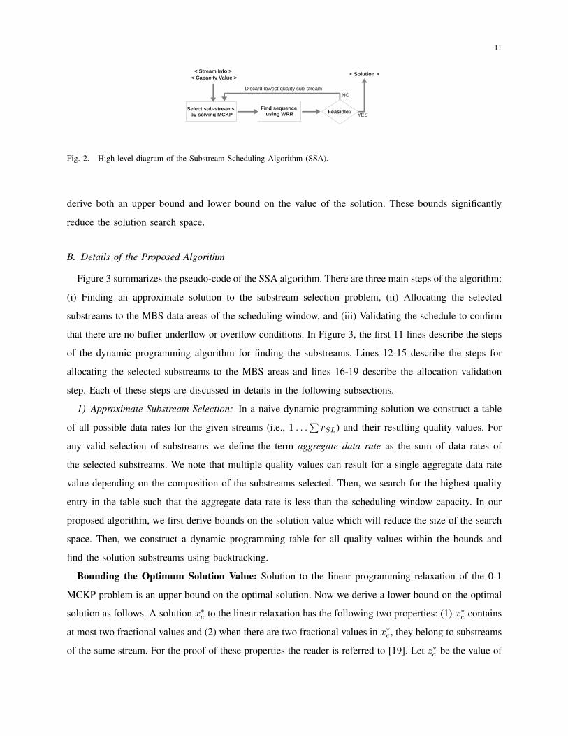
The proposed algorithm is called Substream Selection Algorithm and is denoted by SSA. The high

level idea of the algorithm is depicted in Figure 2 and is described as follows. We first find a set of near

optimal substreams given the data capacity of a scheduling window. Then, we allocate them to the MBS

areas in the frames of the scheduling window. If no feasible allocation is found, we reduce the problem

instance by discarding the substream with lowest quality among all substreams. We solve the optimal

substream selection problem again for the reduced set of substreams. This cycle is repeated until either

a feasible solution is found, or none of the substreams is selected. Once a solution is found the frame

allocation is done in a modified weighted round robin manner.

As shown in Theorem 1, the problem of selecting optimal scalable substreams is similar to solving the

0-1 Multiple Choice Knapsack Problem. This problem has been studied in the mathematical programming

community and several near-optimal solution schemes exist. The reader is referred to the survey by

Lin [18] for a summary of the main results. Dynamic programming is one of the techniques used for

designing approximation algorithms for the 0-1 Multiple Choice Knapsack Problem. However, dynamic

programming solutions are often memory intensive and may involve large constants. In our algorithm we

11

Fig. 2. High-level diagram of the Substream Scheduling Algorithm (SSA).

derive both an upper bound and lower bound on the value of the solution. These bounds significantly

reduce the solution search space.

B. Details of the Proposed Algorithm

Figure 3 summarizes the pseudo-code of the SSA algorithm. There are three main steps of the algorithm:

(i) Finding an approximate solution to the substream selection problem, (ii) Allocating the selected

substreams to the MBS data areas of the scheduling window, and (iii) Validating the schedule to confirm

that there are no buffer underflow or overflow conditions. In Figure 3, the first 11 lines describe the steps

of the dynamic programming algorithm for finding the substreams. Lines 12-15 describe the steps for

allocating the selected substreams to the MBS areas and lines 16-19 describe the allocation validation

step. Each of these steps are discussed in details in the following subsections.

1) Approximate Substream Selection: In a naive dynamic programming solution we construct a table

of all possible data rates for the given streams (i.e., 1 . . .∑

rSL) and their resulting quality values. For

any valid selection of substreams we define the term aggregate data rate as the sum of data rates of

the selected substreams. We note that multiple quality values can result for a single aggregate data rate

value depending on the composition of the substreams selected. Then, we search for the highest quality

entry in the table such that the aggregate data rate is less than the scheduling window capacity. In our

proposed algorithm, we first derive bounds on the solution value which will reduce the size of the search

space. Then, we construct a dynamic programming table for all quality values within the bounds and

find the solution substreams using backtracking.

Bounding the Optimum Solution Value: Solution to the linear programming relaxation of the 0-1

MCKP problem is an upper bound on the optimal solution. Now we derive a lower bound on the optimal

solution as follows. A solution x∗

c to the linear relaxation has the following two properties: (1) x∗

c contains

at most two fractional values and (2) when there are two fractional values in x∗

c , they belong to substreams

of the same stream. For the proof of these properties the reader is referred to [19]. Let z∗c be the value of

12

the objective function corresponding to x∗

c . Let Q0 be the maximum of (a) the objective function value

when both the fractional values are dropped from the solution and (b) maximum of the quality values of

the fractional variables. If the optimal solution for the integer problem is Q∗, it is evident that Q0 ≤ Q∗.

From the properties of x∗

c it is evident that at most two variables are dropped. Since at most two variables

are dropped, z∗c can be bounded as z∗c ≤ 2Q0. Also, since the solution obtained by the linear relaxation

must be greater than or equal to the solution obtained by the integer program, we have an upper bound

on the optimum integer solution as Q0 ≤ Q∗ ≤ z∗c ≤ 2Q0. We note that although the bound is obtained

from linear programming theory, we do not require an LP solver to calculate Q0. Q0 can be calculated

using the median finding algorithms in linear time [20].

Recursive Table Generation: Now that we know the bounds of the optimal solution value we define

a dynamic programming formulation as follows. For all streams s ∈ {1, . . . , S} and all quality values

q ∈, {0 . . . , 2Q0}, we define V (s, q) as the set of substreams from streams 1, . . . , s such that no two

substreams are selected from the same stream and the total quality of the selected substreams is q. If for

a quality value q the at most one substream per stream constraint is violated we set the corresponding

sum of weights to infinity. Let R(s, q) denote the sum of data rates selected in V (s, q). We assume that

the sum of data rates to produce zero quality is zero, i.e., R(s, 0) = 0. Also, for the first stream, the

data rate values can be computed easily as just the data rate of the substream, or the minimum of the

data rates if more than one substream has the same quality, i.e., R(1, q) = minl

{rsl} where qsl = q. In

mathematical terms, the first stream data rates can be expressed as in equation (2a). The data rates for

the other quality values and other streams can be computed by the recursive definition described in (2b)

and the optimum quality can be expressed by equation (2c).

R(1, q) =

minl{rsl}, where l ∈ L and qsl = q,

∞, otherwise.

(2a)

R(s, q) =

min{R(s − 1, q), minl∈L

{rsl

+R(s − 1, q − qsl)}}, when qsl ≤ q,

R(s − 1, q), otherwise.

(2b)

Q∗ = max{q|R(s, q) ≤ PF}. (2c)

However, the size of the table can still be very large as it is bounded only by Q0. Therefore we select a

scaling factor K = ǫQ0/S, and scale down the quality values to q′sl = qsl/K. This operation considerably

reduces the table size while admitting only a small error factor. We bound the quality degradation due

13

to scaling in our mathematical analysis in Section IV-C.

Backtracking: Once we have computed the dynamic programming table, the solution quality value

is obtained by a simple scanning of the table as in equation (2c). The solution substream vectors are

found using a backtracking mechanism as follows. While constructing the recursive table, we store the

composition of substreams leading to the data rates R(s, q) as a list for each table cell. The solution

substream vector is found using the additional information by backtracking from the cell containing the

solution quality value.

2) Data allocation: Once the substreams are selected, it remains to allocate them to the MBS data

area such that the subscriber’s playback buffers do not overflow or underflow. We use a modified version

of the weighted round robin algorithm to allocate data to frames. The weighted round robin has been

used for scheduling constant bit rate traffic before [21]. However, for a variable bit rate stream the stream

priorities are not static. We derive the priority of a stream based on its buffer level at the subscriber. At

the beginning of the scheduling window, for a stream s let the data rate of the selected substream be rs

and the buffer level be Bs. Then stream s is assigned priority Bs/rs. A lower value of Bs/rs denotes

higher priority. We also need to allocate the number of frames to a stream in the current round, that

is, the length of the burst. The burst length is chosen such that none of the other streams suffer from

starvation, nor does it cause overflow or underflow at the receiver buffer. For a stream s the length of

the burst is given by min {Bs/τrs}.

3) Buffer State Validation: After the schedule is constructed, we check if any buffer constraint is

violated. This can be easily determined by verifying the buffer overflow and underflow constraints

described in equations (1c) and (1d). If the buffer constraints are violated, the current substreams cannot

be allocated within the current scheduling window. Hence, we reduce the problem size and re-compute

substreams. The problem size is reduced by discarding the substream with minimum quality value among

all substreams. This process is repeated until a feasible solution is found or none of the substreams is

selected. We note that even though the scheduler is located at the base station, it is aware of the subscriber

buffer size and stream data rates. From this information it can calculate the change in buffer states for a

given schedule without any involvement from the subscribers.

C. Correctness and Performance Analysis

We first prove in Lemma 1 that the data rate and quality values of substreams of a scalable stream

constitute a non-dominated set. In Lemma 2, we prove the correctness of the recursive formulation

described in equations (2a)-(2b). Using Lemma 1 and Lemma 2 we prove the correctness of SSA.

14

Substream Selection Algorithm (SSA)

Input : Substreams, MBS capacity, Frame duration

Scheduling window size

Output : Data burst allocation in the MBS area of

the current scheduling window

1. For each enhancement layer i across all streams do

2. Compute ρi = rsl − rsl−1 and φi = (qsl − qsl−1)

3. Select k largestφi

ρi

such that∑

i∈k

ρi < PF −∑

rs1

4. Determine lower bound Q0 =∑

φi +∑

qs1

5. Compute scale factor K = ǫQ0/S

6. Scale the quality values such that q′sl = qsl

K

7. For q = 1 to 2Q0 do

8. For s = 1 to S do

9. If s is 1, Compute R(s, q) using equation (2a)

10. Else, Compute R(s, q) using equation (2b)

11. Backtrack table R(s, q) to find the substreams s∗

12. Until all streams are allocated do

13. Arrange substreams in ascending order ofBs

rs

14. Allocate σs = min Bs

τrs

frames to stream s

15. Update Bs = Bs + σs ∗ F − σsτrs

16. If no valid allocation found do

17. Find substream (l, s) such that qsl

= mins∈S,l∈L

{qsl}

18. Discard substream (l, s)

19. Go to step 3

Fig. 3. The proposed Substream Selection Algorithm.

15

Lemma 1: Data rates and quality values of substreams extracted from scalable streams constitute non-

dominated set.

Proof: Let l and l′ be two substreams of a given stream s. Substream l is said to be dominated

by substream l′ if including l′ in the solution always leads to better quality than including substream

l. For example, let rsl, r′

sl be the data rates and qsl, q′

sl be the quality values of substreams l and l′. If

rsl > r′sl and qsl < q′sl then l is dominated by l′. Greet et al. [22] have shown that, for the H.264 PSNR

scalability, when there is sufficient variability in a video, its rate-distortion characterization will be close

to a quadratic function which is convex. In our problem, since the streams are variable bit rate videos

and layer encoded, the data rate and quality value pair of the layers within a stream can be assumed to

form a convex set.

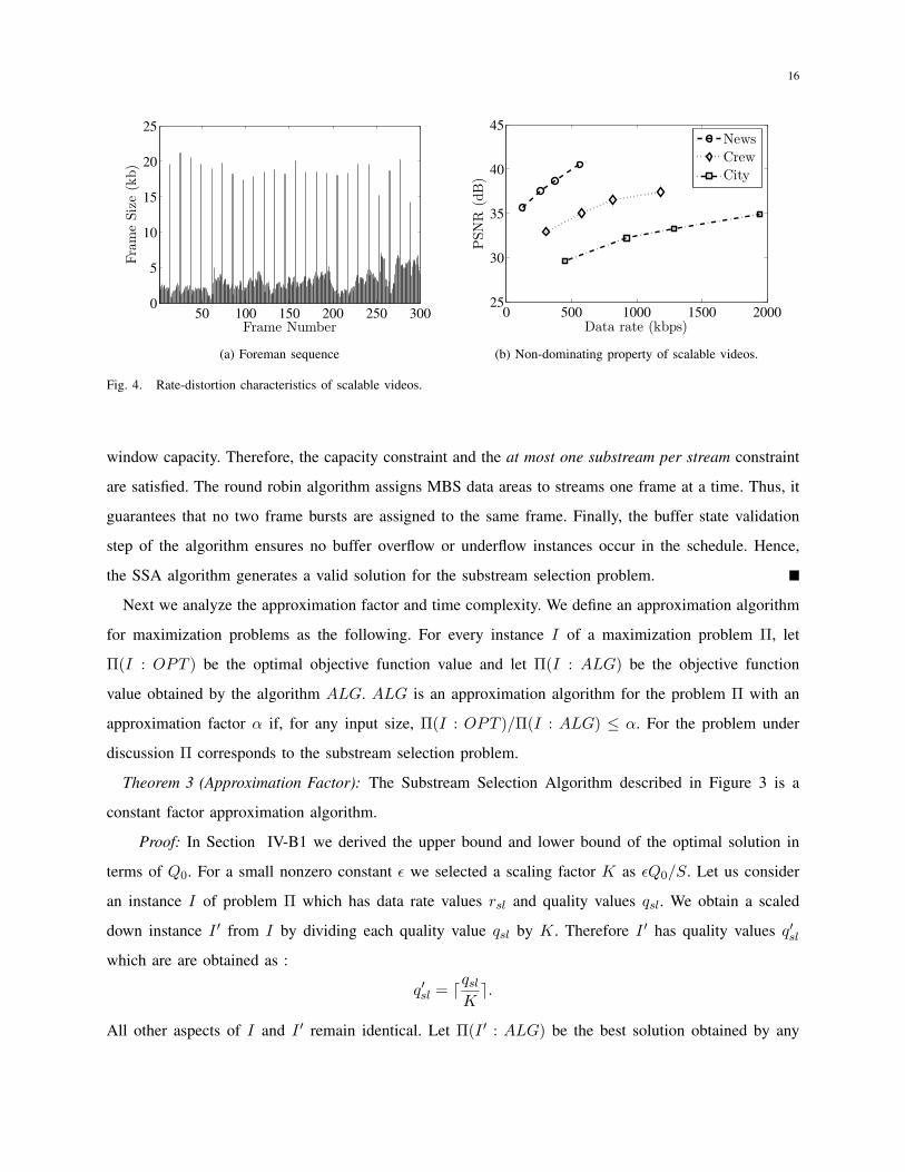
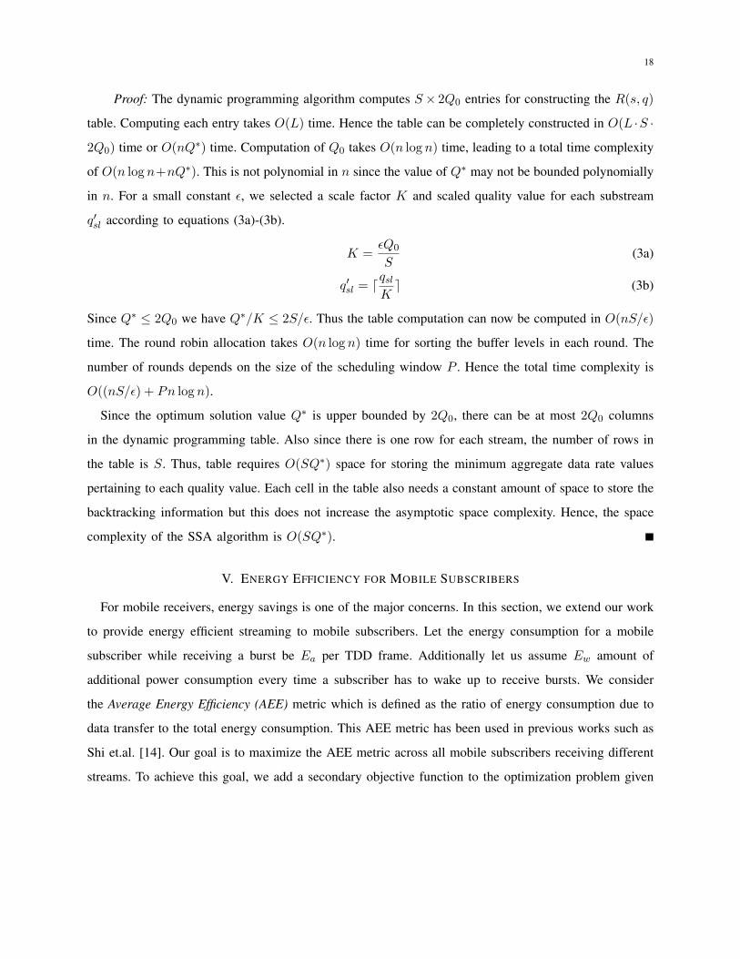
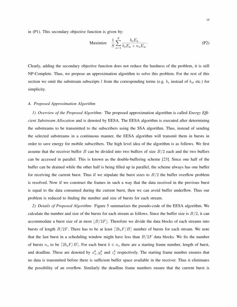
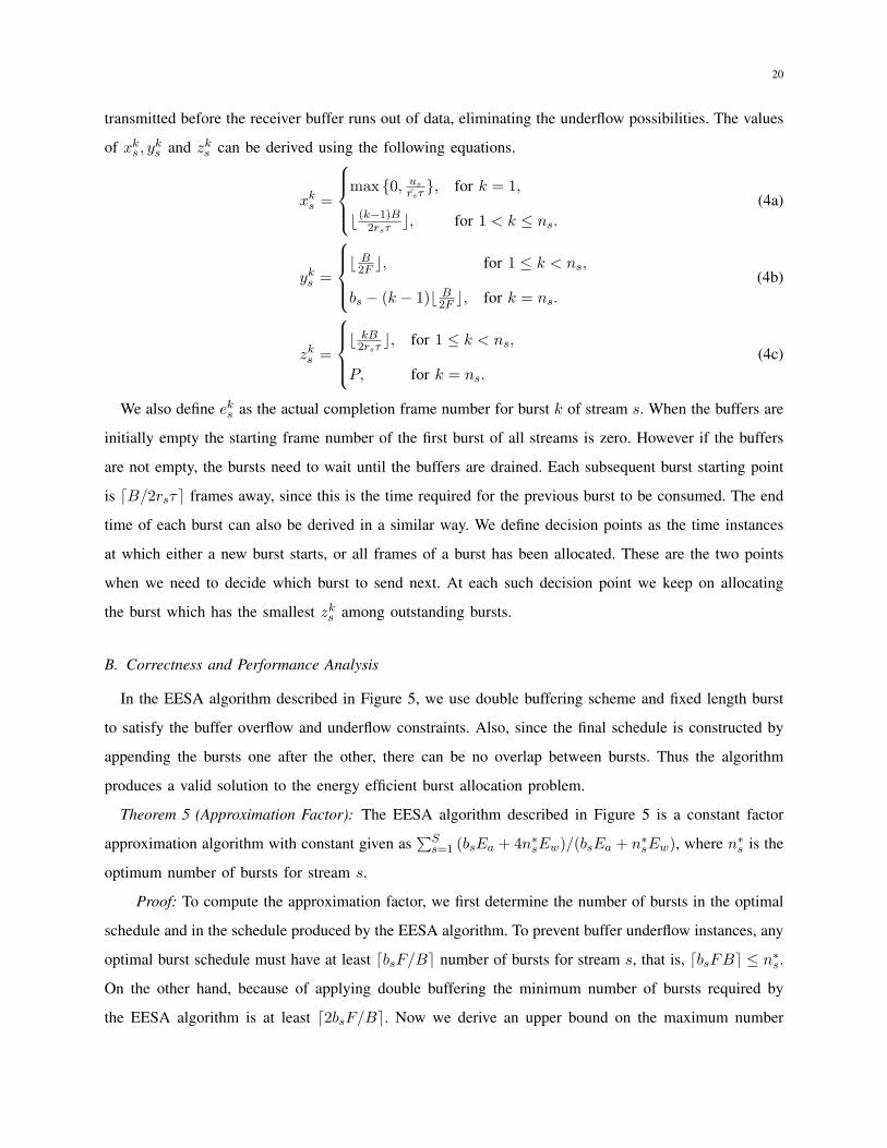
Therefore, Lemma 1 indicates that our problem instances are already in non-dominated form and we

can easily solve the linear relaxation of the best quality substream selection problem. Efficient solution to

the linear relaxation will help us in efficiently computing the final solution value. We empirically validate

the assumption of rate variability and convexity. In Figure 4a we plot the sizes of frames of one of our

test streams to show the high data rate variability. In Figure 4b we plot the data rate and PSNR values

of three test streams and validate that they indeed form a convex envelop.

Lemma 2: The recurrence relations described in equations (2a)-(2c) produce a near optimal substream

selection solution.

Proof: According to Lemma 1, all instances consist of only non-dominated substreams. Thus we

only need to prove the correctness of the recurrence relation. We can prove the correctness of the recursive

expression by induction. The basis step where s = 1 is true since it will lead to the selection of the

maximum quality substream such that the data rate is less than the scheduling window capacity. Now let

us assume that it is also true for the case of s− 1 streams. For stream s the expression R(s− 1, q − qsl)

retrieves the weight of the solution and updates it by adding the current data rate. Then all such data rates

are compared which can result in quality q and only the minimum is chosen. Since R(s−1, q) is already

minimum, this results in R(s, q) also being minimum for every quality value. Since only selections from

the set V (s, q) can have non-infinite values is ensures that only one substream per stream is selected.

Theorem 2 (Correctness): The Substream Selection Algorithm described in Figure 3 returns a valid

solution for the Substream Selection Problem.

Proof: By Lemma 2, the solution to the dynamic programming formulation selects substreams such

that the average quality is close to the optimal and the total data requirement is less than the scheduling

16

50 100 150 200 250 3000

5

10

15

20

25

Frame Number

Fra

me

Siz

e(k

b)

(a) Foreman sequence

0 500 1000 1500 200025

30

35

40

45

Data rate (kbps)

PSN

R(d

B)

News

Crew

City

(b) Non-dominating property of scalable videos.

Fig. 4. Rate-distortion characteristics of scalable videos.

window capacity. Therefore, the capacity constraint and the at most one substream per stream constraint

are satisfied. The round robin algorithm assigns MBS data areas to streams one frame at a time. Thus, it

guarantees that no two frame bursts are assigned to the same frame. Finally, the buffer state validation

step of the algorithm ensures no buffer overflow or underflow instances occur in the schedule. Hence,

the SSA algorithm generates a valid solution for the substream selection problem.

Next we analyze the approximation factor and time complexity. We define an approximation algorithm

for maximization problems as the following. For every instance I of a maximization problem Π, let

Π(I : OPT ) be the optimal objective function value and let Π(I : ALG) be the objective function

value obtained by the algorithm ALG. ALG is an approximation algorithm for the problem Π with an

approximation factor α if, for any input size, Π(I : OPT )/Π(I : ALG) ≤ α. For the problem under

discussion Π corresponds to the substream selection problem.

Theorem 3 (Approximation Factor): The Substream Selection Algorithm described in Figure 3 is a

constant factor approximation algorithm.

Proof: In Section IV-B1 we derived the upper bound and lower bound of the optimal solution in

terms of Q0. For a small nonzero constant ǫ we selected a scaling factor K as ǫQ0/S. Let us consider

an instance I of problem Π which has data rate values rsl and quality values qsl. We obtain a scaled

down instance I ′ from I by dividing each quality value qsl by K. Therefore I ′ has quality values q′sl

which are are obtained as :

q′sl = ⌈qsl

K⌉.

All other aspects of I and I ′ remain identical. Let Π(I ′ : ALG) be the best solution obtained by any

17

algorithm ALG on the scaled down instance I ′ and Π(I ′ : SSA) be the solution obtained by our SSA

algorithm. Since we rounded up the quality values during the scaling operation we have

Π(I : ALG) ≤ Π(I ′ : ALG).

Also, since our algorithm finds the optimum solution for the scaled down problem, we have

Π(I ′ : ALG) ≤ Π(I ′ : SSA).

From the above two equations we have

Π(I : ALG) ≤ Π(I ′ : SSA).

Now, since each quality value in the solution of Π(I ′ : SSA) is at most K times bigger than the quality

values in solution of Π(I : SSA), and we can have only S number of such quality values in a valid

solution we have

Π(I : ALG) ≤ Π(I ′ : SSA) ≤ Π(I : SSA) + SK.

Replacing the value of K we have

Π(I : ALG) ≤ Π(I : SSA) + ǫQ0.

Now, since Q0 is a lower bound to our solution we have

Π(I : SSA) + ǫQ0 ≤ Π(I : SSA) + ǫΠ(I : SSA).

From the above two equations we have,

Π(I : ALG) ≤ (1 + ǫ)Π(I : SSA).

ALG can be any algorithm including OPT , the optimal algorithm. Therefore we have,

Π(I : OPT )

Π(I : SSA)≤ (1 + ǫ).

In other words, the solution obtained by the SSA algorithm is always with a factor of (1 + ǫ) of the

optimal algorithm for every instance I of the problem Π. Therefore the SSA algorithm is a constant

factor approximation algorithm with approximation factor (1 + ǫ).

Theorem 4 (Time and Space Complexity): The SSA algorithm in Figure 3 has a time complexity of

O((nS/ǫ)+Pn log n), where n = O(∑

L) is the total number of substreams, L is the maximum number

of substreams within a stream, P is the scheduling window size, and ǫ > 0 is a small constant. The

space complexity is O(SQ∗), where S is the number of streams and Q∗ is the optimum quality value

18

Proof: The dynamic programming algorithm computes S × 2Q0 entries for constructing the R(s, q)

table. Computing each entry takes O(L) time. Hence the table can be completely constructed in O(L ·S ·

2Q0) time or O(nQ∗) time. Computation of Q0 takes O(n log n) time, leading to a total time complexity

of O(n log n+nQ∗). This is not polynomial in n since the value of Q∗ may not be bounded polynomially

in n. For a small constant ǫ, we selected a scale factor K and scaled quality value for each substream

q′sl according to equations (3a)-(3b).

K =ǫQ0

S(3a)

q′sl = ⌈qsl

K⌉ (3b)

Since Q∗ ≤ 2Q0 we have Q∗/K ≤ 2S/ǫ. Thus the table computation can now be computed in O(nS/ǫ)

time. The round robin allocation takes O(n log n) time for sorting the buffer levels in each round. The

number of rounds depends on the size of the scheduling window P . Hence the total time complexity is

O((nS/ǫ) + Pn log n).

Since the optimum solution value Q∗ is upper bounded by 2Q0, there can be at most 2Q0 columns

in the dynamic programming table. Also since there is one row for each stream, the number of rows in

the table is S. Thus, table requires O(SQ∗) space for storing the minimum aggregate data rate values

pertaining to each quality value. Each cell in the table also needs a constant amount of space to store the

backtracking information but this does not increase the asymptotic space complexity. Hence, the space

complexity of the SSA algorithm is O(SQ∗).

V. ENERGY EFFICIENCY FOR MOBILE SUBSCRIBERS

For mobile receivers, energy savings is one of the major concerns. In this section, we extend our work

to provide energy efficient streaming to mobile subscribers. Let the energy consumption for a mobile

subscriber while receiving a burst be Ea per TDD frame. Additionally let us assume Ew amount of

additional power consumption every time a subscriber has to wake up to receive bursts. We consider

the Average Energy Efficiency (AEE) metric which is defined as the ratio of energy consumption due to

data transfer to the total energy consumption. This AEE metric has been used in previous works such as

Shi et.al. [14]. Our goal is to maximize the AEE metric across all mobile subscribers receiving different

streams. To achieve this goal, we add a secondary objective function to the optimization problem given

19

in (P1). This secondary objective function is given by:

Maximize1

S

S∑

s=1

bsEa

bsEa + nsEw

. (P2)

Clearly, adding the secondary objective function does not reduce the hardness of the problem, it is still

NP-Complete. Thus, we propose an approximation algorithm to solve this problem. For the rest of this

section we omit the substream subscripts l from the corresponding terms (e.g. bs instead of bsl etc.) for

simplicity.

A. Proposed Approximation Algorithm

1) Overview of the Proposed Algorithm: The proposed approximation algorithm is called Energy Effi-

cient Substream Allocation and is denoted by EESA. The EESA algorithm is executed after determining

the substreams to be transmitted to the subscribers using the SSA algorithm. Thus, instead of sending

the selected substreams in a continuous manner, the EESA algorithm will transmit them in bursts in

order to save energy for mobile subscribers. The high level idea of the algorithm is as follows. We first

assume that the receiver buffer B can be divided into two buffers of size B/2 each and the two buffers

can be accessed in parallel. This is known as the double-buffering scheme [23]. Since one half of the

buffer can be drained while the other half is being filled up in parallel, the scheme always has one buffer

for receiving the current burst. Thus if we stipulate the burst sizes to B/2 the buffer overflow problem

is resolved. Now if we construct the frames in such a way that the data received in the previous burst

is equal to the data consumed during the current burst, then we can avoid buffer underflow. Thus our

problem is reduced to finding the number and size of bursts for each stream.

2) Details of Proposed Algorithm: Figure 5 summarizes the pseudo-code of the EESA algorithm. We

calculate the number and size of the bursts for each stream as follows. Since the buffer size is B/2, it can

accommodate a burst size of at most ⌊B/2F ⌋. Therefore we divide the data blocks of each streams into

bursts of length B/2F . There has to be at least ⌈2bsF/B⌉ number of bursts for each stream. We note

that the last burst in a scheduling window might have less than B/2F data blocks. We fix the number

of bursts ns to be ⌈2bsF/B⌉. For each burst k ∈ ns there are a starting frame number, length of burst,

and deadline. These are denoted by xks , y

ks and zk

s respectively. The starting frame number ensures that

no data is transmitted before there is sufficient buffer space available in the receiver. Thus it eliminates

the possibility of an overflow. Similarly the deadline frame numbers ensure that the current burst is

20

transmitted before the receiver buffer runs out of data, eliminating the underflow possibilities. The values

of xks , y

ks and zk

s can be derived using the following equations.

xks =

max {0, us

rsτ}, for k = 1,

⌊ (k−1)B2rsτ

⌋, for 1 < k ≤ ns.

(4a)

yks =

⌊ B2F

⌋, for 1 ≤ k < ns,

bs − (k − 1)⌊ B2F

⌋, for k = ns.

(4b)

zks =

⌊ kB2rsτ

⌋, for 1 ≤ k < ns,

P, for k = ns.

(4c)

We also define eks as the actual completion frame number for burst k of stream s. When the buffers are

initially empty the starting frame number of the first burst of all streams is zero. However if the buffers

are not empty, the bursts need to wait until the buffers are drained. Each subsequent burst starting point

is ⌈B/2rsτ⌉ frames away, since this is the time required for the previous burst to be consumed. The end

time of each burst can also be derived in a similar way. We define decision points as the time instances

at which either a new burst starts, or all frames of a burst has been allocated. These are the two points

when we need to decide which burst to send next. At each such decision point we keep on allocating

the burst which has the smallest zks among outstanding bursts.

B. Correctness and Performance Analysis

In the EESA algorithm described in Figure 5, we use double buffering scheme and fixed length burst

to satisfy the buffer overflow and underflow constraints. Also, since the final schedule is constructed by

appending the bursts one after the other, there can be no overlap between bursts. Thus the algorithm

produces a valid solution to the energy efficient burst allocation problem.

Theorem 5 (Approximation Factor): The EESA algorithm described in Figure 5 is a constant factor

approximation algorithm with constant given as∑S

s=1 (bsEa + 4n∗

sEw)/(bsEa + n∗

sEw), where n∗

s is the

optimum number of bursts for stream s.

Proof: To compute the approximation factor, we first determine the number of bursts in the optimal

schedule and in the schedule produced by the EESA algorithm. To prevent buffer underflow instances, any

optimal burst schedule must have at least ⌈bsF/B⌉ number of bursts for stream s, that is, ⌈bsFB⌉ ≤ n∗

s.

On the other hand, because of applying double buffering the minimum number of bursts required by

the EESA algorithm is at least ⌈2bsF/B⌉. Now we derive an upper bound on the maximum number

21

Energy Efficient Substream Allocation (EESA)

Input : Selected substreams, Initial buffer values,

Scheduling window size

Output : Data burst allocation in the MBS area of

the current scheduling window

1. For s = 1 to S do

3. Determine ns = ⌈2bsF/B⌉

4. For k = 1 to ns do

5. Determine xks , yk

s , and zks using Equations (4a)-(4c)

6. Let Λ = ∅

7. For each decision point do

8. Add a burst from frames tc to tn to stream s, where wks

9. has the smallest zks among outstanding bursts, tc

10. is current time, and tn is time of the next decision point

11. Let eks be the actual finish time of burst k

12. If max{eks − zk

s } ≤ 0 // complete on time

13. Return Λ

14. Return no feasible schedule

Fig. 5. Energy Efficient Substream Allocation Algorithm

of bursts that can be constructed by algorithm the EESA. From the definition of the decision points,

each burst derived by equations (4a)-(4c) can cause at most one interruption in rest of the bursts. This

happens when all frames of the current burst are not allocated but the current frame number is the

starting frame number of a different burst. Therefore these interruptions may cause additional ⌈2bsF/B⌉

number of bursts for the EESA algorithm. Therefore the maximum number of bursts created by the EESA

algorithm is 2(⌈2bsF/B⌉), in other words, ns ≤ 4⌈bsF/B⌉. Comparing this with the value of n∗

s we

have ns ≤ 4n∗

s. The approximation factor can be given as the AEE achieved by the optimal algorithm

to that achieved by our EESA algorithm. Ignoring the common terms in both expressions we have the

following approximation factor.

AEE (OPT)

AEE (EESA)=

S∑

s=1

bsEa + 4n∗

sEw

bsEa + n∗sEw

. (5)

22

We note that since the number of bursts in the optimal solution n∗

s is a constant, the approximation factor

is also constant.

The allocation algorithm for mobile subscribers, EESA, involves a sorting of the bursts to assign their

priorities. Since the number of bursts depends on the length of the scheduling window, sorting takes

O(P log P ) time. Therefore the overall running time of the algorithm EESA is O(SP log P ).

VI. TRACE-DRIVEN EVALUATION

A. Simulation Setup

We have implemented a point-to-multipoint WiMAX multimedia broadcast simulator and evaluated

our algorithm in it using actual scalable video traces. For the WiMAX network parameters we use the

16-QAM modulation scheme with 3/4 convolution turbo coding and 10MHz channel. Since each TDD

frame is 5ms, for a one second scheduling window we will have to allocate data to 200 TDD frames.

Also we assume that within each TDD frame we have an MBS data area of 50kb. This gives us a

broadcast channel bandwidth of 10Mbps [24]. At the receiver side we assume a buffer limit of 512kb.

For generating the video traffic we use 10 raw (YUV files in 4:2:0 format) video files from the video

trace repository of Arizona State University [25]. For each video we generate a 10 minute workload by

starting from a random initial frame and then repeating the frame sequences. Then we encode the videos

into H.264/SVC format using the JSVM reference software version 9.18 [26]. We encode each stream

into four PSNR scalable layers using the medium grain scalability (MGS) feature of the H.264/SVC

coding standard [17]. We tune the encoding parameters such that the substreams have average bit rate

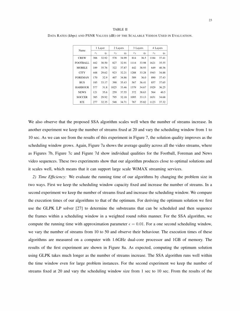
between 100kbps and 2.5Mbps. In Table II, we summarize the information of the data rates and quality

values of each layer of the different video files.

B. Simulation Results

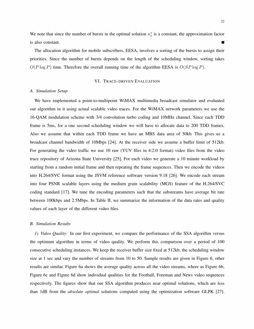
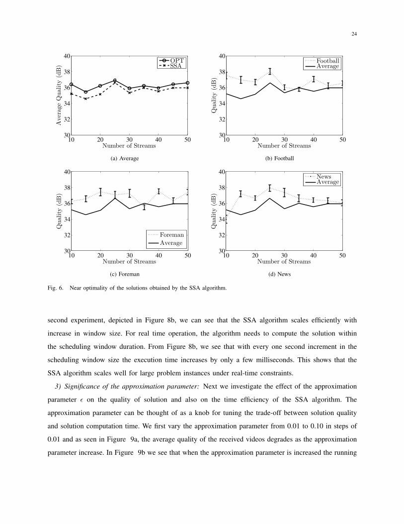
1) Video Quality: In our first experiment, we compare the performance of the SSA algorithm versus

the optimum algorithm in terms of video quality. We perform this comparison over a period of 100

consecutive scheduling instances. We keep the receiver buffer size fixed at 512kb, the scheduling window

size at 1 sec and vary the number of streams from 10 to 50. Sample results are given in Figure 6; other

results are similar. Figure 6a shows the average quality across all the video streams, where as Figure 6b,

Figure 6c and Figure 6d show individual qualities for the Football, Foreman and News video sequences

respectively. The figures show that our SSA algorithm produces near optimal solutions, which are less

than 1dB from the absolute optimal solutions computed using the optimization software GLPK [27].

23

TABLE II

DATA RATES (kbps) AND PSNR VALUES (dB) OF THE SCALABLE VIDEOS USED IN EVALUATION.

Name1 Layer 2 Layers 3 Layers 4 Layers

r1 q1 r2 q2 r3 q3 r4 q4

CREW 306 32.92 578 34.99 814 36.5 1184 37.41

FOOTBALL 442 30.50 827 32.91 1114 33.98 1621 35.55

MOBILE 189 35.76 322 37.87 442 38.93 649 40.36

CITY 448 29.62 923 32.21 1288 33.28 1943 34.88

FOREMAN 170 32.9 407 34.86 589 36.0 890 37.43

BUS 185 33.17 390 35.43 567 36.41 857 37.65

HARBOUR 577 31.8 1025 33.46 1379 34.67 1929 36.25

NEWS 121 35.6 259 37.55 372 38.63 564 40.5

SOCCER 385 29.92 795 32.18 1095 33.13 1651 34.68

ICE 277 32.35 548 34.71 767 35.82 1123 37.32

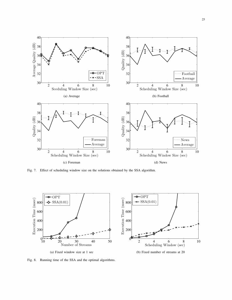
We also observe that the proposed SSA algorithm scales well when the number of streams increase. In

another experiment we keep the number of streams fixed at 20 and vary the scheduling window from 1 to

10 sec. As we can see from the results of this experiment in Figure 7, the solution quality improves as the

scheduling window grows. Again, Figure 7a shows the average quality across all the video streams, where

as Figures 7b, Figure 7c and Figure 7d show individual qualities for the Football, Foreman and News

video sequences. These two experiments show that our algorithm produces close to optimal solutions and

it scales well, which means that it can support large scale WiMAX streaming services.

2) Time Efficiency: We evaluate the running time of our algorithms by changing the problem size in

two ways. First we keep the scheduling window capacity fixed and increase the number of streams. In a

second experiment we keep the number of streams fixed and increase the scheduling window. We compare

the execution times of our algorithms to that of the optimum. For deriving the optimum solution we first

use the GLPK LP solver [27] to determine the substreams that can be scheduled and then sequence

the frames within a scheduling window in a weighted round robin manner. For the SSA algorithm, we

compute the running time with approximation parameter ǫ = 0.01. For a one second scheduling window,

we vary the number of streams from 10 to 50 and observe their behaviour. The execution times of these

algorithms are measured on a computer with 1.6GHz dual-core processor and 1GB of memory. The

results of the first experiment are shown in Figure 8a. As expected, computing the optimum solution

using GLPK takes much longer as the number of streams increase. The SSA algorithm runs well within

the time window even for large problem instances. For the second experiment we keep the number of

streams fixed at 20 and vary the scheduling window size from 1 sec to 10 sec. From the results of the

24

10 20 30 40 5030

32

34

36

38

40

Number of Streams

Aver

age

Quality

(dB

)

OPTSSA

(a) Average

10 20 30 40 5030

32

34

36

38

40

Number of Streams

Quality

(dB

)

FootballAverage

(b) Football

10 20 30 40 5030

32

34

36

38

40

Number of Streams

Qual

ity

(dB

)

Foreman

Average

(c) Foreman

10 20 30 40 5030

32

34

36

38

40

Number of Streams

Qual

ity

(dB

)

NewsAverage

(d) News

Fig. 6. Near optimality of the solutions obtained by the SSA algorithm.

second experiment, depicted in Figure 8b, we can see that the SSA algorithm scales efficiently with

increase in window size. For real time operation, the algorithm needs to compute the solution within

the scheduling window duration. From Figure 8b, we see that with every one second increment in the

scheduling window size the execution time increases by only a few milliseconds. This shows that the

SSA algorithm scales well for large problem instances under real-time constraints.

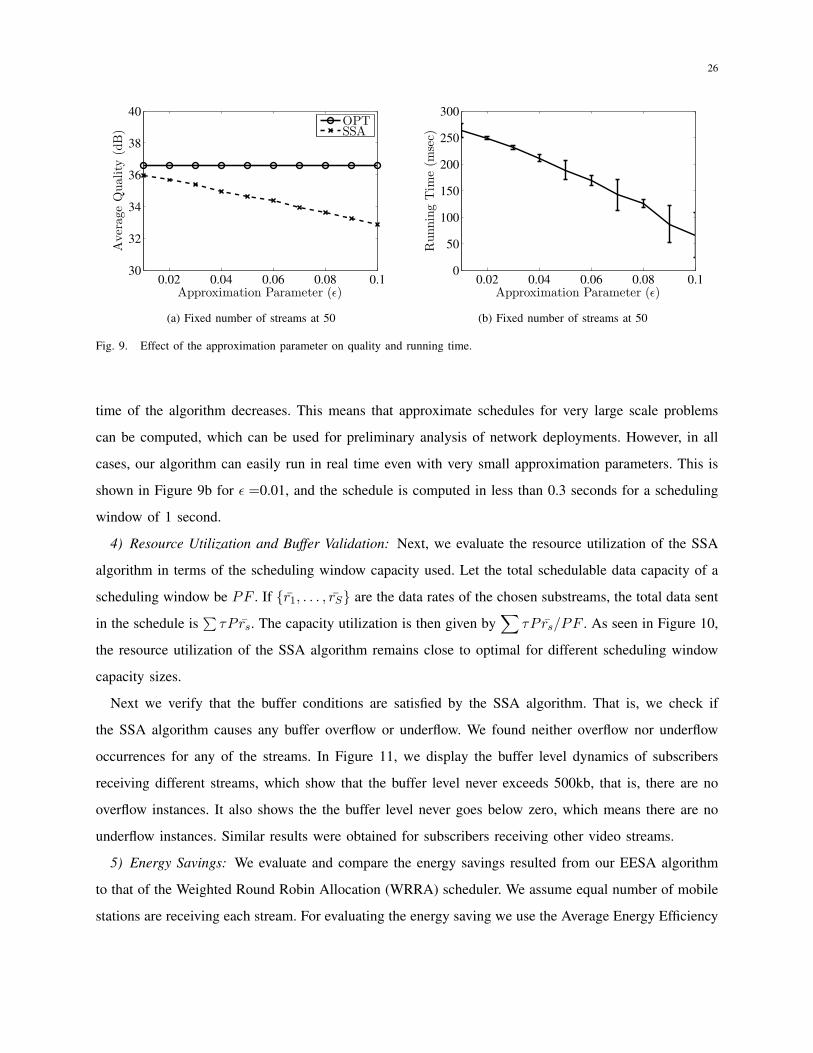
3) Significance of the approximation parameter: Next we investigate the effect of the approximation

parameter ǫ on the quality of solution and also on the time efficiency of the SSA algorithm. The

approximation parameter can be thought of as a knob for tuning the trade-off between solution quality

and solution computation time. We first vary the approximation parameter from 0.01 to 0.10 in steps of

0.01 and as seen in Figure 9a, the average quality of the received videos degrades as the approximation

parameter increase. In Figure 9b we see that when the approximation parameter is increased the running

25

2 4 6 8 1030

32

34

36

38

40

Sceduling Window Size (sec)

Aver

age

Quality

(dB

)

OPT

SSA

(a) Average

2 4 6 8 1030

32

34

36

38

40

Scheduling Window Size (sec)

Quality

(dB

)

Football

Average

(b) Football

2 4 6 8 1030

32

34

36

38

40

Scheduling Window Size (sec)

Qual

ity

(dB

)

Foreman

Average

(c) Foreman

2 4 6 8 1030

32

34

36

38

40

Scheduling Window Size (sec)

Qual

ity

(dB

)

News

Average

(d) News

Fig. 7. Effect of scheduling window size on the solutions obtained by the SSA algorithm.

10 20 30 40 500

200

400

600

800

Number of Streams

Exec

uti

onT

ime

(mse

c)

OPT

SSA(0.01)

(a) Fixed window size at 1 sec

2 4 6 8 100

200

400

600

800

Scheduling Window (sec)

Exec

uti

onT

ime

(mse

c)

OPT

SSA(0.01)

(b) Fixed number of streams at 20

Fig. 8. Running time of the SSA and the optimal algorithms.

26

0.02 0.04 0.06 0.08 0.130

32

34

36

38

40

Approximation Parameter (ǫ)

Aver

age

Quality

(dB

)

OPTSSA

(a) Fixed number of streams at 50

0.02 0.04 0.06 0.08 0.10

50

100

150

200

250

300

Approximation Parameter (ǫ)

Runnin

gT

ime

(mse

c)

(b) Fixed number of streams at 50

Fig. 9. Effect of the approximation parameter on quality and running time.

time of the algorithm decreases. This means that approximate schedules for very large scale problems

can be computed, which can be used for preliminary analysis of network deployments. However, in all

cases, our algorithm can easily run in real time even with very small approximation parameters. This is

shown in Figure 9b for ǫ =0.01, and the schedule is computed in less than 0.3 seconds for a scheduling

window of 1 second.

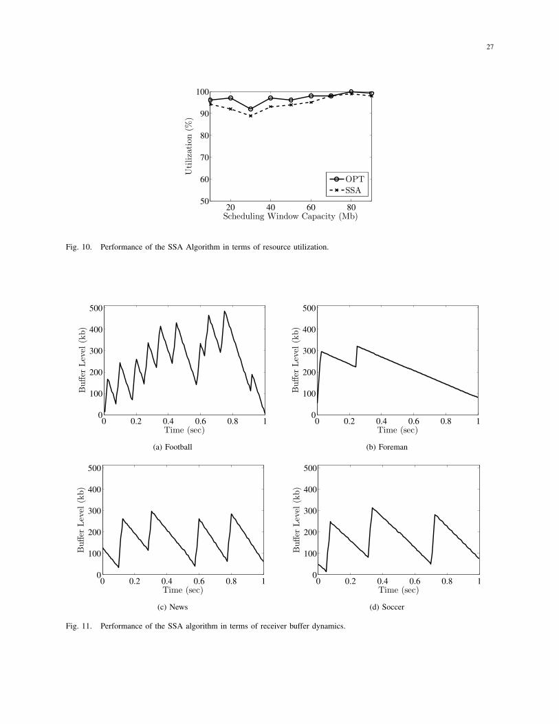
4) Resource Utilization and Buffer Validation: Next, we evaluate the resource utilization of the SSA

algorithm in terms of the scheduling window capacity used. Let the total schedulable data capacity of a

scheduling window be PF . If {r1, . . . , rS} are the data rates of the chosen substreams, the total data sent

in the schedule is∑

τP rs. The capacity utilization is then given by∑

τP rs/PF . As seen in Figure 10,

the resource utilization of the SSA algorithm remains close to optimal for different scheduling window

capacity sizes.

Next we verify that the buffer conditions are satisfied by the SSA algorithm. That is, we check if

the SSA algorithm causes any buffer overflow or underflow. We found neither overflow nor underflow

occurrences for any of the streams. In Figure 11, we display the buffer level dynamics of subscribers

receiving different streams, which show that the buffer level never exceeds 500kb, that is, there are no

overflow instances. It also shows the the buffer level never goes below zero, which means there are no

underflow instances. Similar results were obtained for subscribers receiving other video streams.

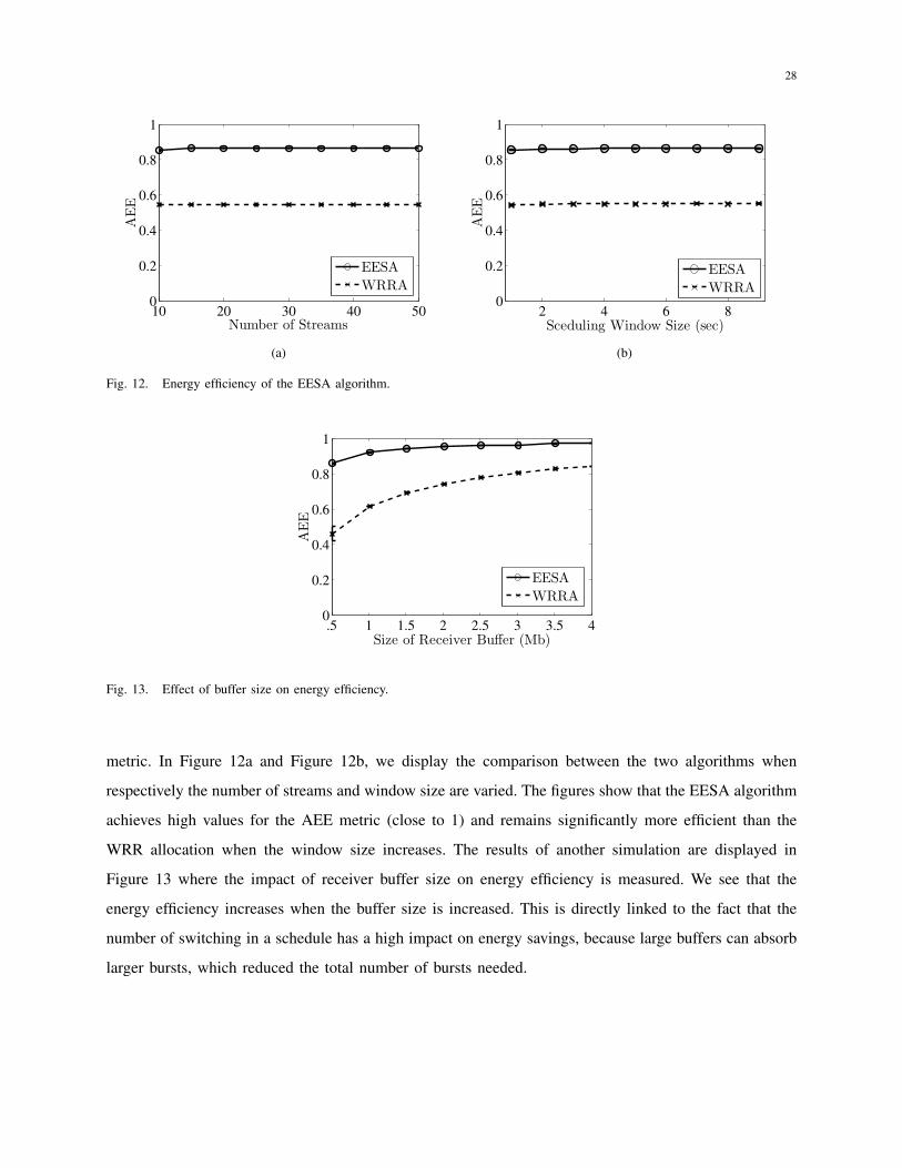
5) Energy Savings: We evaluate and compare the energy savings resulted from our EESA algorithm

to that of the Weighted Round Robin Allocation (WRRA) scheduler. We assume equal number of mobile

stations are receiving each stream. For evaluating the energy saving we use the Average Energy Efficiency

27

20 40 60 8050

60

70

80

90

100

Scheduling Window Capacity (Mb)

Uti

liza

tion

(%)

OPT

SSA

Fig. 10. Performance of the SSA Algorithm in terms of resource utilization.

0 0.2 0.4 0.6 0.8 10

100

200

300

400

500

Time (sec)

Buffer

Lev

el(k

b)

(a) Football

0 0.2 0.4 0.6 0.8 10

100

200

300

400

500

Time (sec)

Buffer

Lev

el(k

b)

(b) Foreman

0 0.2 0.4 0.6 0.8 10

100

200

300

400

500

Time (sec)

Buffer

Lev

el(k

b)

(c) News

0 0.2 0.4 0.6 0.8 10

100

200

300

400

500

Time (sec)

Buffer

Lev

el(k

b)

(d) Soccer

Fig. 11. Performance of the SSA algorithm in terms of receiver buffer dynamics.

28

10 20 30 40 500

0.2

0.4

0.6

0.8

1

Number of Streams

AE

E

EESA

WRRA

(a)

2 4 6 80

0.2

0.4

0.6

0.8

1

Sceduling Window Size (sec)

AE

E

EESA

WRRA

(b)

Fig. 12. Energy efficiency of the EESA algorithm.

.5 1 1.5 2 2.5 3 3.5 40

0.2

0.4

0.6

0.8

1

Size of Receiver Buffer (Mb)

AE

E

EESA

WRRA

Fig. 13. Effect of buffer size on energy efficiency.

metric. In Figure 12a and Figure 12b, we display the comparison between the two algorithms when

respectively the number of streams and window size are varied. The figures show that the EESA algorithm

achieves high values for the AEE metric (close to 1) and remains significantly more efficient than the

WRR allocation when the window size increases. The results of another simulation are displayed in

Figure 13 where the impact of receiver buffer size on energy efficiency is measured. We see that the

energy efficiency increases when the buffer size is increased. This is directly linked to the fact that the

number of switching in a schedule has a high impact on energy savings, because large buffers can absorb

larger bursts, which reduced the total number of bursts needed.

29

VII. CONCLUSIONS AND FUTURE WORK

We presented a framework for multicasting scalable video streams over mobile WiMAX networks.

We mathematically analyzed the problem of selecting the optimal substreams of scalable video streams

under bandwidth constraints. Solving this problem is important because it enables the network operator

to transmit higher-quality videos or more number of video streams at the same capacity. We showed that

the substream selection problem in presence of bandwidth limitation is NP-Complete. We proposed a

novel approximation algorithm for this problem. We proved that our algorithm has a small approximation

factor of (1 + ǫ), and it has a time complexity of O(nS/ǫ), where n = O(∑

L) is the total number of

layers, and L is the maximum number of layers in a scalable stream. We implemented and validated

our algorithm in a simulation setup and studied the impact of a wide range of parameters using multiple

video traces. Our simulation results show that the approximation factor of the proposed algorithm is very

close to one for practical scenarios. We also verified that our algorithm can run in real time and that

it scales well to large scheduling problems. In addition, we extended our formulation to consider the

energy constraints of mobile receivers. We presented an algorithm to transmit the data in bursts in order

to conserve energy of mobile receivers. Using simulation, we showed that our algorithm achieves high

energy savings.

The work in this paper can be extended in different directions. For example, we are currently extending

our algorithm to consider the probability distribution of hardware profiles of active receivers. The algo-

rithm takes into account the diverse parameters like buffer size, display resolution and energy consumption

profiles such that, the produced solution not only optimize the video quality but also enhances the quality

of experience for the majority of mobile subscribers.

REFERENCES

[1] Mobile Video Services: A Five-Year Global Market Forecast, “http://www.pyr.com/store/RPMOBILEVIDEOSERV0906.

htm.”

[2] Open Mobile Video Coalition website, “http://www.openmobilevideo.com/resources/omvc-materials/reports/.”

[3] IEEE Standard, “Local and metropolitan area networks Part 16: Air Interface for Broadband Wireless Access Systems

Broadband Wireless Metropolitan Area Network ,” http://standards.ieee.org/getieee802/802.16.html.

[4] Yota Mobile WiMAX Home Page, “http://www.yota.ru/en/info/main/.”

[5] UDCAST WiMAX TV Home Page, “http://www.udcast.com/products/udcast wimax tv products.htm.”

[6] S. Sharangi, R. Krishnamurti, and M. Hefeeda, “Streaming Scalable Video over WiMAX Networks,” in Proc. of IEEE

Workshop on Quality of Service (IWQoS’10), Beijing, China, June 2010, (to appear).

[7] J. Wang, M. Venkatachalam, and Y. Fang, “System architecture and cross-layer optimization of video broadcast over

WiMAX,” IEEE Journal on Selected Areas in Communications, vol. 25, no. 4, pp. 712–721, May 2007.

30

[8] R. Cohen, L. Katzir, and R. Rizzi, “On the trade-off between energy and multicast efficiency in 802.16e-like mobile

networks,” IEEE Transactions on Mobile Computing, vol. 7, no. 3, pp. 346–357, March 2008.

[9] P. Hosein, “Broadcasting VBR traffic in a WiMAX network,” in Proc. of IEEE VTC’08, Calgary, Canada, September 2008,

pp. 1–5.

[10] H. Juan, H. Huang, C. Huang, and T. Chiang, “Scalable video streaming over mobile WiMAX,” in Proc. of International

Symposium on Circuits and Systems, New Orleans, LA, May 2007, pp. 3463–3466.

[11] V. Reguant, F. Prats, R. de Pozuelo, F. Margalef, and G. Ubiergo, “Delivery of H.264 SVC/MDC streams over WiMAX

and DVB-T networks,” in Proc. of IEEE International Symposium on Consumer Electronics (ISCE’08), Algarve, Portugal,

April 2008, pp. 1–4.

[12] J. Seo, S. Lee, N. Park, H. Lee, and C. Cho, “Performance analysis of sleep mode operation in IEEE 802.16e,” in Proc.

of IEEE VTC’04, Los Angeles, CA, September 2004, pp. 1169–1173.

[13] M. Kim, M. Kang, and J. Choi, “Remaining Energy-Aware Power Management Mechanism in the 802.16e MAC,” in Proc.

of IEEE Consumer Communications and Networking Conference (CCNC’08), Las Vegas,NV, January 2008, pp. 222–226.

[14] J. Shi, G. Fang, Y. Sun, J. Zhou, Z. Li, and E. Dutkiewicz, “Improving Mobile Station Energy Efficiency in IEEE 802.16e

WMAN by Burst Scheduling,” in Proc. of IEEE GLOBECOM’06, San Francisco, CA, December 2006, pp. 1–5.

[15] W. Liao and N. Lee, “An Integrated Power Saving Scheduling Algorithm in 802.16e Wireless Metropolitan Area Networks,”

in Proc. of International Conference on Mobile Technology, Applications & Systems, Yilan, Taiwan, 2008, pp. 1–8.

[16] M. Garey and D. Johnson, Computers and Intractability: A guide to the Theory of NP-Completeness. W. H. Freeman

and Company, 1979.

[17] T. Wiegand, G. Sullivan, G. Bjøntegaard, and A. Luthra, “Overview of the H.264/AVC Video Coding Standard,” IEEE

Transactions on Circuits and Systems for Video Technology, vol. 13, no. 7, pp. 560–576, July 2003.

[18] E. Lin, “A bibliographical survey on some well-known non-standard knapsack problems,” Information Systems and

Operation Research, vol. 36, pp. 274–317, November 1998.

[19] A. Sinha and A. Zoltners, “The multiple-choice knapsack problem,” Operations Research, vol. 27, no. 3, pp. 503–515,

June 1979.

[20] E. Zemel, “An O(n) Algorithm for the linear multiple choice knapsack problem and related problems,” Information

Processing Letters, vol. 18, no. 3, pp. 123–128, March 1984.

[21] P. Hosein and T. Gopal, “Radio resource management for broadcast services in OFDMA-based networks,” in Proc. of

IEEE International Conference on Communications Workshops, Beijing, China, May 2008, pp. 271–275.

[22] V. Geert, P. David, M. Reisslein, and L. Karam, “Traffic and quality characterization of the H.264/AVC scalable video

coding extension,” Advances in MultiMedia, vol. 2008, no. 2, pp. 1–27, January 2008.

[23] C. Hsu and M. Hefeeda, “Time Slicing in Mobile TV Broadcast Networks with Arbitrary Channel Bit Rates,” in Proc. of

IEEE INFOCOM’09, Rio de Janeiro, Brazil, April 2009, pp. 2231–2239.

[24] D. Gray, “Mobile WiMAX Part I - Overview and Performance,” WiMAX Forum, White Paper, August 2006, available

online at www.wimaxforum.org/technology/downloads/Mobile WiMAX Part1 Overview and Performance.pdf.

[25] Arizona State University: Video Traces Research Group, “http://trace.eas.asu.edu.”

[26] Fraunhofer HHI: JSVM H.264 AVC/SVC Reference Software, “http://ip.hhi.de/imagecom G1/savce/downloads/

SVC-Reference-Software.htm.”

[27] GNU Linear Programming Kit, “http://www.gnu.org/software/glpk/glpk.html.”